Identification of Wetland Conservation Gaps in Rapidly Urbanizing Areas: A Case Study in Zhengzhou, China

Abstract

Exploring protected area (PA) siting from a biodiversity perspective is critical in mitigating human impacts on ecosystems. This paper used the MaxEnt model to predict the geographic distribution patterns of wetland species in Zhengzhou and the environmental factors affecting species’ habitat selection. Environmental variables were screened by correlation analysis to avoid affecting the prediction results due to overfitting of the model. The AUC value of the training set of the model ROC curve was above 0.8, and the prediction accuracy was high. The prediction results showed that the only nature reserve in Zhengzhou, Yellow River Wetland Nature Reserve, currently covers only 10.25% of the total area of the high suitability areas for plants and 17.54% of the high suitability habitat areas for waterfowl in the whole area of Zhengzhou. The potential suitability areas of wetland species outside the reserve can provide a basis for site selection for wetland conservation planning in Zhengzhou. It was found that the geographic distribution of wetland species in Zhengzhou is constrained by the distribution of water bodies, bioclimatic variables, land cover, and population density.

1. Introduction

Although artificial wetlands cannot replace the ecological functions provided by natural wetlands [1], as natural wetlands diminish with demand for agriculture or urbanization, artificial wetlands in urban environments become increasingly crucial for wetland species such as waterfowl [2]. As a city’s most biodiversity-rich ecosystem, wetlands are facing a series of problems, such as decreasing scale and weakening functions due to climate change and urbanization. Starting in the 19th century, establishing protected areas became a meaningful way to mitigate and respond to the negative impacts of human activities on global ecosystems [3]. Data from the State Forestry and Grassland Administration show that China has established more than 10 types of protected areas, such as nature reserves, scenic spots, forest parks, and geoparks, with the number of more than 10,000, covering about 18% of the land area. However, with development and urbanization, the problems of spatial fragmentation and conservation gaps have become more prominent in nature reserve systems, and many important wetlands are not fully protected. The rapid expansion of urbanization has caused damage to wetland ecosystems that is difficult to reverse and costly to repair. Therefore, the construction of national ecological civilization has put forward new requirements for wetland protection planning. On 24 December 2021, the thirty-second meeting of the Standing Committee of the thirteenth National People’s Congress adopted the Wetland Protection Law of the People’s Republic of China. It is proposed that the objectives, tasks, general layout, protection, restoration priorities, and guarantee measures of wetland protection planning should be clarified.

Maintaining species diversity is one of the essential priorities for the designation of wetland reserves [4]. Understanding biodiversity characteristics in rapidly urbanizing environments is vital to maintaining the stability of urban ecosystems [5]. In previous studies, species occurrence and distribution data have been widely used to inform the construction of PA networks [6]. The easiest way to incorporate this information is to use point data directly, i.e., the locations where the species of interest were recorded. These data may come from a variety of sources: museum records and surveys, collections of botanical specimens or—in the case of point distribution data—online databases [7]. However, a strength of point data is their availability, and increasingly point distribution data are available through online databases. However, point data is also highly susceptible to errors, such as inaccurate geographic coordinates or taxonomic records, misidentification of species, or incorrect taxonomic nomenclature. In addition, some species’ presence records may only relate to contemporaneous conditions [8]. Indeed, no area has complete point data [9], and some species present may not be detected during extensive surveys, thus making it almost impossible to investigate the entire possible range of most species in detail.

Species distribution models (SDMs) [10] provide one way to overcome the typical sparsity of distributional data by associating them with a set of geographic or environmental predictors. Conceptually addressing errors caused by inadequate sampling and observations, the statistical analysis of the relationships between occurrence and mapped environmental predictors is usually based on records of species presence or abundance. Maps are often created to show differences in the geographical suitability of single species [11,12]. The currently applied species distribution modeling methods include: Ecological Niche Factor Analysis (ENFA), Generalised Linear Model (GLM) [13] or Generalised Additive Model, GAM), the BIOCLIM species distribution modeling package [14], the HABITAT and DOMAIN procedures [15], and the maximum entropy model. Additionally, there are other methods. Among the non-regression methods, BIOCLIM was the first widely used SDM package [16] and is based on the principle of relating the bioclimatic envelope of a species to the range of many bioclimatic variables. DOMAIN, on the other hand, uses a similarity measure to give an index of applicability of the prediction by calculating the minimum distance to any presence record in the environment [17]. However, models that rely on simple relational descriptions and variable weights tend to perform relatively poorly in simulating current species distributions due to the complexity factor of species’ responses to the environment [18]. In contrast, the maximum entropy model simulates the potential spatial distribution pattern of a species by exploring [19], firstly, the non-random relationship between the environmental characteristics of the species in its known range [20,21] and, secondly, its potential habitat. This is achieved by using two available data collections: the actual distribution of the species, and environmental variables [22,23].

The application of SDMs plays an essential role in quantifying species’ environmental and ecological niches [24], evaluating species distribution in response to land use and other ecological changes, and supporting conservation planning and PA selection [10]. However, SDMs have been used less frequently in conservation planning [25,26]. Planning activities are often conducted without involving an end-user or a stakeholder [27]. This has led to questions about the utility of many conservation planning-related studies. In recent years, Zhengzhou Municipal Party Committee and Municipal Government began to pay attention to ecological construction as an important way to promote sustainable economic and social development in Zhengzhou City.

In this study, the influence of bioclimatic and geographic factors on urban wetland species was modeled based on the “MaxEnt” maximum entropy algorithm. Potential habitats for wetland species were classified into four classes: unsuitable, low, moderate, and high. By overlaying high suitability habitats with existing wetland reserves, the conservation gap areas of urban wetlands in Zhengzhou were initially identified. It provides a site selection basis for the conservation of urban wetlands and can lead to environmentally friendly urban development and wetland conservation by local governments.

2. Materials and Methods

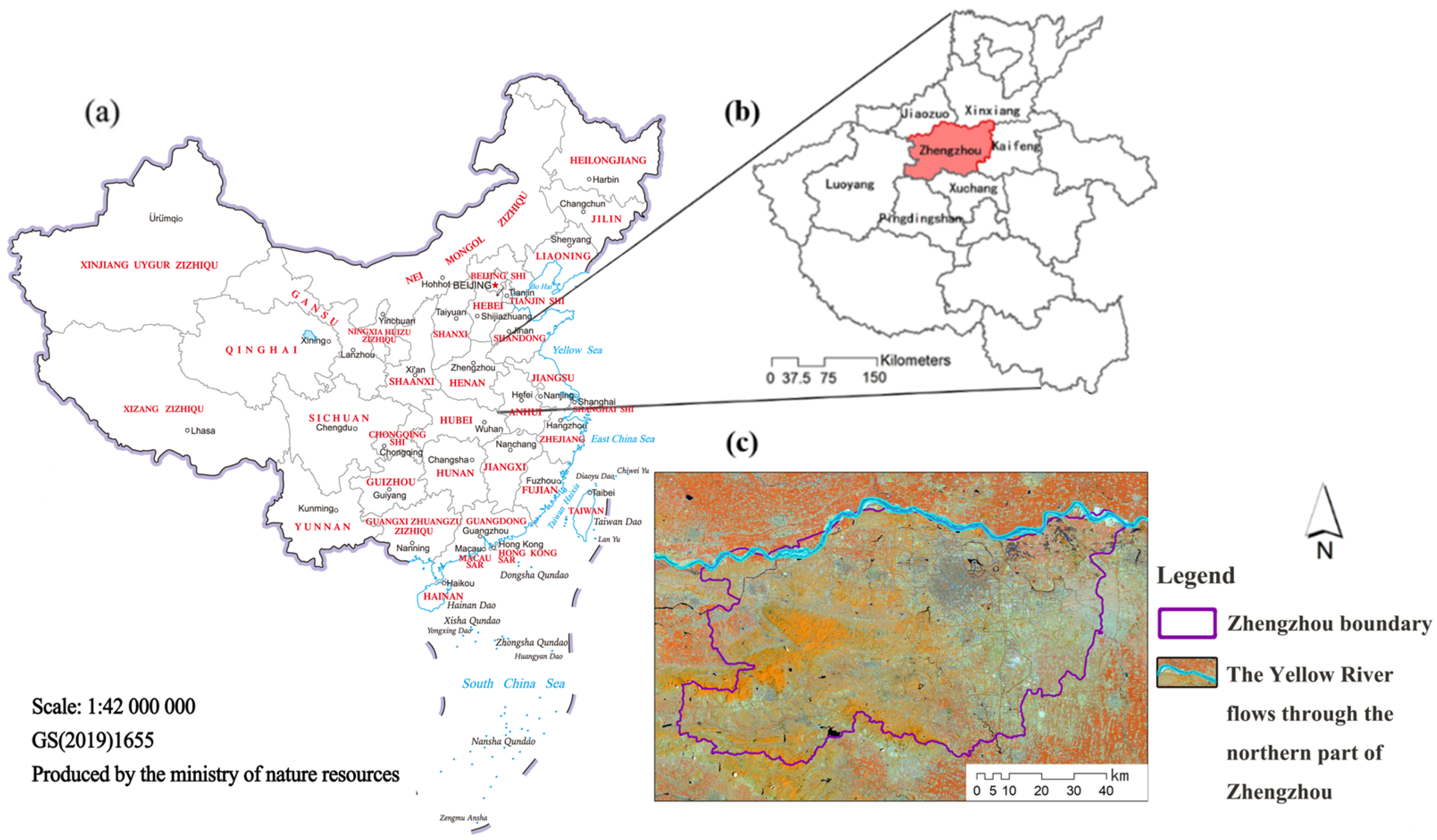
2.1. Study Area

There are two main reasons for choosing Zhengzhou as the study area. First, Zhengzhou (34.7466° N, 113.6253° E) is one of the fastest-growing cities in China in terms of urbanization [28]. In 2000, the built-up area of Zhengzhou was only 133 km². Under the influence of urban population growth and driving policy factors, the built-up area of Zhengzhou has doubled in size since 2002, when construction of the Zhengdong New District began [27]. Secondly, Zhengzhou is located in the middle and lower reaches of the Yellow River, meaning its wetlands are situated in the middle of three major migratory channels in China. This location is an important place for wild birds and, especially, winter migratory birds, specifically for wintering, resting, and feeding (Figure 1).

In 2018, the Zhengzhou City Wetland Resources Protection Master Plan (2019–35) was prepared by the Municipal Forestry Bureau with the support of the municipal government. This resulted in a guarantee between the built and natural environment, with wetlands recognized as an environmental resource whilst still supporting the development of urban construction. A field survey of species resources was conducted by Henan Agricultural University. This paper is one outcome of the survey and provides a scientific basis for conservation planning.

2.2. Data Source and Processing

2.2.1. Records of Wetland Plants and Waterfowl Occurrence in Zhengzhou

Spatial data on wetland plant distribution were obtained from the 2018 Zhengzhou wetland resource survey. Additionally, waterfowl occurrence records were combined with the 2018 Zhengzhou bird survey and verifiable distribution data from the iNaturalist data platform (https://www.inaturalist.org/ (accessed on 26 August 2021)). The wetland dominant plant communities survey is based on the “National Wetland Resources Survey and Technical Regulations (for Trial Implementation)” and the relevant provisions of the “Zhengzhou Wetland Protection Regulations”. The survey was conducted in August by a total of 76 investigators divided into 18 teams. The vegetation survey lines and sample plots were laid out according to the distribution map of water systems. The census was conducted using the sample line method and sample method. Three hundred and twenty-three wetland plant diversity survey sample points were selected for the survey, and 533 2 m × 2 m sample squares were set. Waterfowl surveys are conducted by direct counting method within the survey area. When a waterbird is recorded in any observation zone of a survey site, the survey site is considered to be the distribution point of that species of waterbird.

Most species distribution modeling approaches require spatially independent occurrence record data input. However, researchers often introduce spatially autocorrelated data into SDMs, reducing the ability of the model to predict spatially independent data [29] and leading to results such as model overfitting or amplifying performance values [30]. Therefore, eliminating spatial aggregation of sample locations is essential for model calibration and evaluation. In this paper, the spatially distributed data filter ‘Spatially Rarefy Occurrence Data for SDMs’ (reduce spatial autocorrelation) in the SDM toolbox was first used to dilute the data within one km [30] of other data points. After filtering the data in this way, 211 wetland plant distribution points and 108 waterfowl distribution points remained.

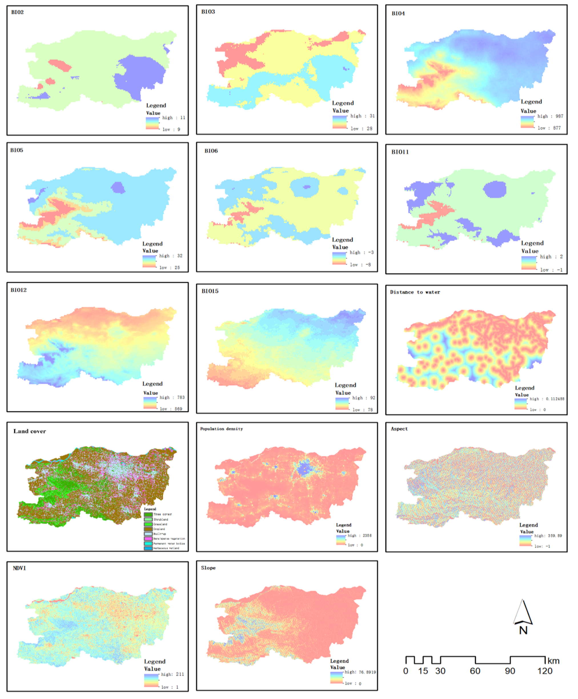
2.2.2. Environmental Variables

According to the references and the current situation of Zhengzhou City, a total of 27 environmental variables were initially selected, including 19 bioclimatic variables; three topographic variables (elevation, slope, and slope direction); two land cover variables (land cover type and normalized vegetation index); two habitat suitability variables (distance to roads and distance to water bodies); and one population density variable.

• Bioclimatic variables

The bioclimatic variables data were derived from WorldClim Global Climate Data version 2.0, which has a spatial resolution of approximately 1 km². The data include monthly temperature (minimum, maximum, and average); precipitation; and 19 other bioclimatic factors (

Table 1. Names and units of bioclimatic variables.

No.	Variable Name	Units
BIO1	Annual Mean Temperature	(°C)
BIO2	Mean Diurnal Range (Mean of monthly (max temp–min temp))	(°C)
BIO3	Isothermality (BIO2/BIO7) (×100)
BIO4	Temperature Seasonality (standard deviation ×100)	C of V
BIO5	Max Temperature of Warmest Month	(°C)
BIO6	Min Temperature of Coldest Month	(°C)
BIO7	Temperature Annual Range (BIO5-BIO6)	(°C)
BIO8	Mean Temperature of Wettest Quarter	(°C)
BIO9	Mean Temperature of Driest Quarter	(°C)
BIO10	Mean Temperature of Warmest Quarter	(°C)
BIO11	Mean Temperature of Coldest Quarter	(°C)
BIO12	Annual Precipitation	(mm)
BIO13	Precipitation of Wettest Month	(mm)
BIO14	Precipitation of Driest Month	(mm)
BIO15	Precipitation Seasonality (Coefficient of Variation)	C of V
BIO16	Precipitation of Wettest Quarter	(mm)
BIO17	Precipitation of Driest Quarter	(mm)
BIO18	Precipitation of Warmest Quarter	(mm)
BIO19	Precipitation of Coldest Quarter	(mm)

). The weather station data was interpolated by using thin slab samples and MODIS satellite data to improve the prediction accuracy of the temperature variables by 5–15% [31]. WorldClim data have been shown to be important predictors of species distribution in a variety of studies.

• Topographical variables

Topographic data were taken from the NASA DEM Digital Elevation Model (DEM) released on 13 February 2020, which has a resolution of 30 m. The 3D Analyst in ArcGIS 10.8 was used to extract the slope direction (Aspect) and slope.

• Land cover variables

The land use data was derived from the 10 m resolution land cover data for 2020 (WorldCover v100) published by the European Space Agency (ESA) [32].The land use classification has an overall accuracy of 74.4%, which is higher than similar publicly available data products. This data provides 11 land cover categories (8 in the study area) defined by using the Land Cover Classification System (LCCS) and developed by the Food and Agriculture Organization of the United Nations with the codes and classifications (

Table A1. Land cover categories in the study area.

Code	Land Cover Categories	LCCS Code	Definition
10	Tree cover	A12A3//A11A1 fA24A3C1(C2)-R1(R2)	Any geographic area dominated by trees, with a cover of 10% or more, land existing under a tree canopy, areas planted for afforestation purposes and plantations, the category also includes areas covered by trees, seasonal or permanent freshwater irrigation, except for mangroves.
20	Shrubland	A12A4//A11A2	Any geographic area dominated by natural shrubs with a cover of 10% or more. Shrubs were defined as woody perennials without a clear main stem, less than 5 m in height, with persistent and lignified stems.
30	Grassland	A12A2	This category includes any geographic area dominated by natural herbaceous plants, including grasslands, pastures, etc., with a cover of 10% or more.
40	Cropland	A11A3(A4)(A5)//A23	Land covered with annual tillage can be harvested at least once within 12 months of the seeding/planting date. Annual cropland produces herbaceous cover, sometimes in combination with some trees or woody vegetation. Note that perennial woody crops will be classified as the appropriate type of tree cover or shrub land cover.
50	Built-up	B15A1	Land covered by buildings, roads and other man-made structures (e.g., railroads), buildings including residential and industrial buildings, urban green spaces (parks, sports facilities) are not included in this category, and waste dumps and extraction sites are considered wastelands.
60	Bare/sparse vegetation	B16A1(A2)//B15A2	Land with bare soil, sand or rock that does not have more than 10% vegetation cover at any time of the year.
80	Permanent water bodies	B28A1(B1)//B27A1(B1)	This category includes any geographic area covered by a body of water for most of the year (more than 9 months), lakes, reservoirs and rivers, which can be fresh or brackish, and in some cases the water is frozen for part of the year (less than 9 months).
90	Herbaceous wetland	A24A2	Land dominated by natural herbaceous vegetation (10% cover or more), permanently or periodically inundated by fresh, brackish or salt water.

) [33]. The study area includes the following land classes: tree cover, shrubland, grassland, cropland, built-up, bare/sparse vegetation, permanent water bodies, and herbaceous wetland.

The normalized difference vegetation index (NDVI) is an important indicator for the ecological environment in spatial planning. The NDVI can be used for global and regional ecological monitoring and simulation, vegetation phenology analysis and information extraction, vegetation cover pattern and change, cropland replanting and crop identification classification, etc. The NDVI quantifies the value of vegetation by measuring the difference between near-infrared band reflectance and red band reflectance. It is calculated as follows:

$$\mathrm{NDVI}=\frac{\left(\mathrm{NIR}-\mathrm{Red}\right)}{\left(\mathrm{NIR}+\mathrm{Red}\right)}$$

(1)

NIR is the near-infrared band reflectance, and Red is the red band reflectance. When Red is lower than the NIR, it means that the area to be measured has dense green vegetation or healthy vegetation growth; when Red is approximately equal to the NIR, it means that the vegetation growth is very poor or no vegetation, and the ground cover is rocky, bare soil, water body, or urban built-up area; when Red is greater than the NIR, it means that there is no vegetation. The NDVI data were obtained from the United States Geological Survey (USGS) website (http://glovis.usgs.gov/ (accessed on 26 August 2021)), a Landsat 8/OLI land surface reflectance product [34].

• Habitat suitability variables

The river network distribution and road network data were obtained from the OpenStreetMap platform (https://www.openstreetmap.org/ (accessed on 30 August 2021)), which provides good coverage of water systems and roads in the study area. We used the Spatial Analyst tool in ArcGIS 10.8 to extract the Euclidean distance from each pixel to the nearest river and road.

• Population density variables

The population density in the year 2020 was obtained from the WorldPop open space population dataset (https://www.worldpop.org/ (accessed on 2 February 2022)), which has a resolution of 1 km.

In ArcGIS 10.8, we preprocessed all raster data by resampling them into a 30 m × 30 m raster with the same number of rows and columns. To avoid multicollinearity among the variables involved in the prediction and, thus, to affect the model prediction results, the initial model was first constructed by using 27 environmental variables to derive the contribution of each factor (

Table A2. Raster plot of all variables involved in the model predictions.

Wetland Plant		Waterfowl
Variables	Percent Contribution	Variables	Percent Contribution
Distance to water	46.3	Distance to water	34.8
BIO4	14.7	Land cover	14
DEM	7.5	BIO5	12
NDVI	4.2	Population density	10.5
Population density	3.6	BIO10	3.4
BIO12	2.5	BIO12	2.7
Aspect	2.4	BIO15	2.7
Land cover	2.4	Distance to road	2.6
BIO16	2.1	BIO18	2.2
BIO2	2	Aspect	2.1
BIO10	1.9	NDVI	1.7
BIO1	1.6	Slope	1.3
Slope	1.5	BIO1	1.3
BIO11	1.1	Dem	1.1
BIO5	0.9	BIO2	1.1
Distance to road	0.8	BIO14	0.9
BIO14	0.7	BIO17	0.8
BIO13	0.7	BIO11	0.7
BIO3	0.7	BIO4	0.7
BIO9	0.6	BIO7	0.6
BIO6	0.5	BIO3	0.5
BIO7	0.5	BIO19	0.4
BIO8	0.4	BIO16	0.4
BIO15	0.3	BIO6	0.4
BIO17	0.2	BIO8	0.4
BIO18	0.1	BIO9	0.3
BIO19	0.1	BIO13	0.3

). The correlation coefficients between 27 raster variables were calculated using the ‘raster.cor.matrix()’ function in the ‘ENMTools’ R package [35], and the groups of variables with correlation coefficients greater than 0.7 were visualized by using the ‘Virtualspecies’ package (Figure 2) [36]. Finally, 12 environmental variables (Figure A1) with significant relative contribution, low correlation, and more apparent ecological significance were screened for each species to inform the model prediction (

Table 2. Screening of the environmental factors that contribute most to the model and are not relevant.

Wetland Species	Bioclimatic Variables	Topography, Land Cover, Habitat Suitability, and Population Density Variables
Wetland plants	BIO4	Distance to water
	BIO12	NDVI
	BIO2	Population density
	BIO11	Aspect
	BIO3	Land cover
	BIO6	Slope
Waterfowl	BIO5	Distance to water
	BIO12	Land cover
	BIO15	Population density
	BIO2	Aspect
	BIO11	NDVI
	BIO3	Slope

A detailed explanation of the bioclimatic variables is explained in Table 1.

) [37].

2.3. Model Selection and Construction

Among SDM-based models, MaxEnt runs only require access to species occurrence point information and environmental data. Among all models that satisfy the constraints, the result with the highest entropy value is selected to predict the species distribution. The maximum entropy model can also effectively handle complex interactions between variables; is more tolerant of small samples, non-regular sampling, and point data with a small amount of bias; and has excellent model prediction performance [38].

Selected environmental layers and occurrence locations of waterfowls and wetland plants were imported into MaxEnt in CSV and ASCII formats for modeling operations. The model parameters were selected as 25% of the distribution points as the test set and 75% of the distribution points as the training set using the ‘crossvalidate’ method (Crossvalidate, dividing the species distribution data into 10 equal parts, selecting 1 part each time as the test set and the remaining 9 parts as the training set, running 10 times repeatedly, with higher data utilization) with the default setting of the maximum number of iterations of 500 and the maximum number of background point numbers is 10,000 [39]; the rest select the default settings, and the final output ASCII result file is the average of 10 repetitive runs [40]. After completing the run, the result file was imported into ArcGIS 10.8 software. The degree of habitability was classified into four classes: unsuitable, low, moderate, and high suitability habitat areas [41]. To identify wetlands, the potential geographical distribution of plants and waterfowl in Zhengzhou City was determined.

2.4. Model Accuracy Evaluation

The subject operating characteristic curve (ROC) was used to test the simulation prediction effect. The area under curve (AUC) value was used as the model prediction measure, and the ROC curve used each value of the prediction result as the possible judgment threshold. The corresponding sensitivity and specificity are calculated with the false positive rate (1 specificity) as the horizontal coordinate and the true positive rate (sensitivity) as the vertical coordinate. Since the AUC value is not affected by the judgment threshold, it can be used to compare different models and therefore becomes the best measure of model accuracy [40]. The AUC takes values between 0 and 1. The closer the AUC is to 1, the better the prediction is. The criteria for judging the prediction model from the AUC are: 0.7–0.8 is more accurate, 0.8–0.9 is very accurate, and 0.9–1.0 is highly precise [42].

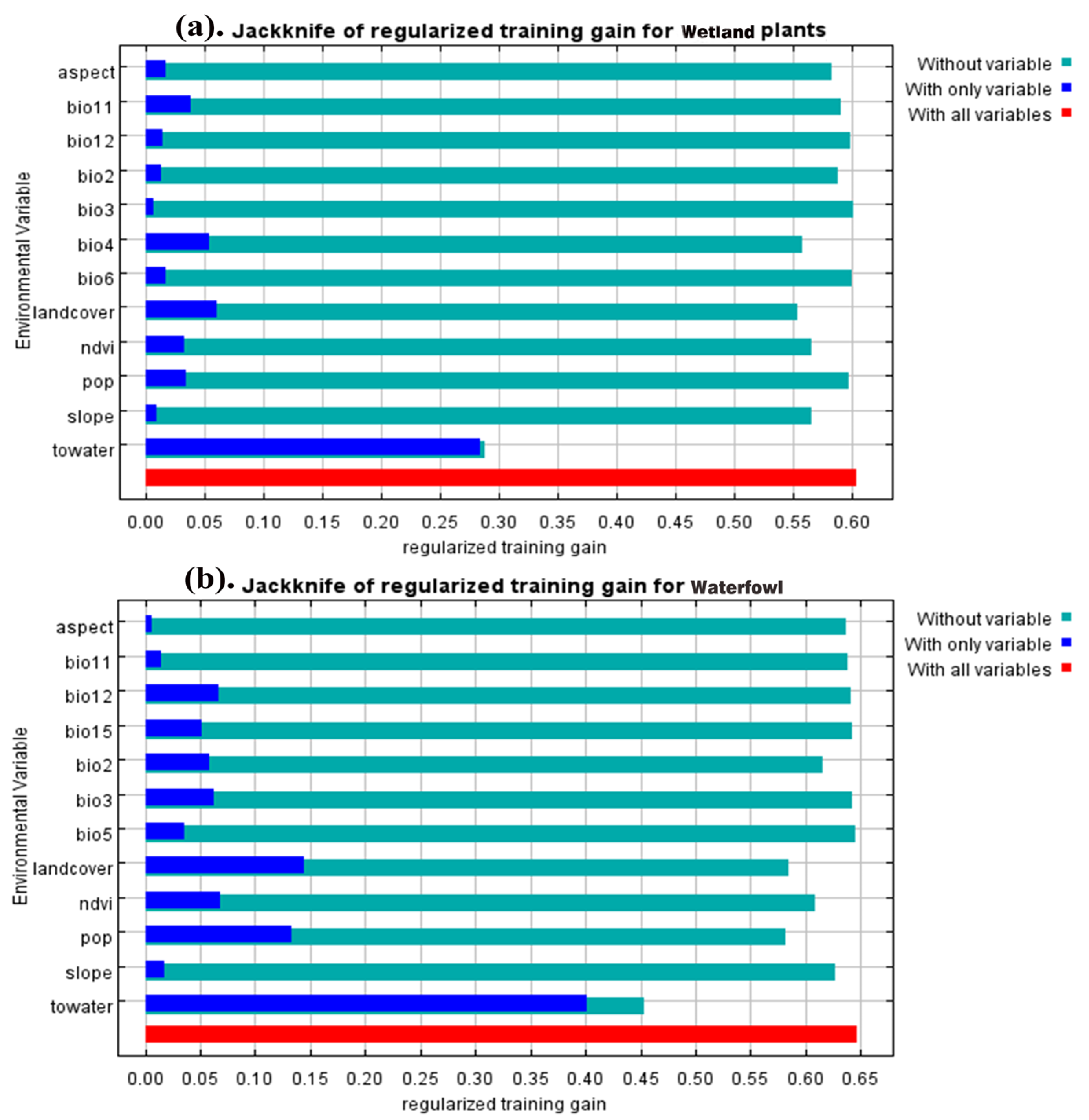
2.5. Importance Assessment of Environmental Variables

MaxEnt modeling aims to measure which variables are the most important for the distribution of species in the model. The first approach is to understand the model’s gain by modifying the coefficients of individual features at each step of the model construction process of the MaxEnt algorithm through relative contribution (percent contribution) and replacement importance (permutation importance), where an increase in the regularization gain is added to the contribution of the corresponding variable at each iteration of the training algorithm and subtracted from it if the change in the absolute value of lambda is negative. In turn, for each environmental variable, the values of that variable in the training presence and background data were randomly ranked. The program assigns the increase in gain to the environmental variables on which the feature values depend and converts them into percentages.

The results of the Jackknife test can reflect the contribution of different environmental variables to the gain of the distribution and determine the contribution of individual factors to the model by calculating the scores of “this variable only”, “except this variable”, and all variables in the simulation, respectively [43]. The higher score for “only this variable” reflecting more contribution of individual variables to the gain in species distribution; the lower score for the “except this variable” scenario suggests that this variable is more important to the species distribution gains.

3. Results

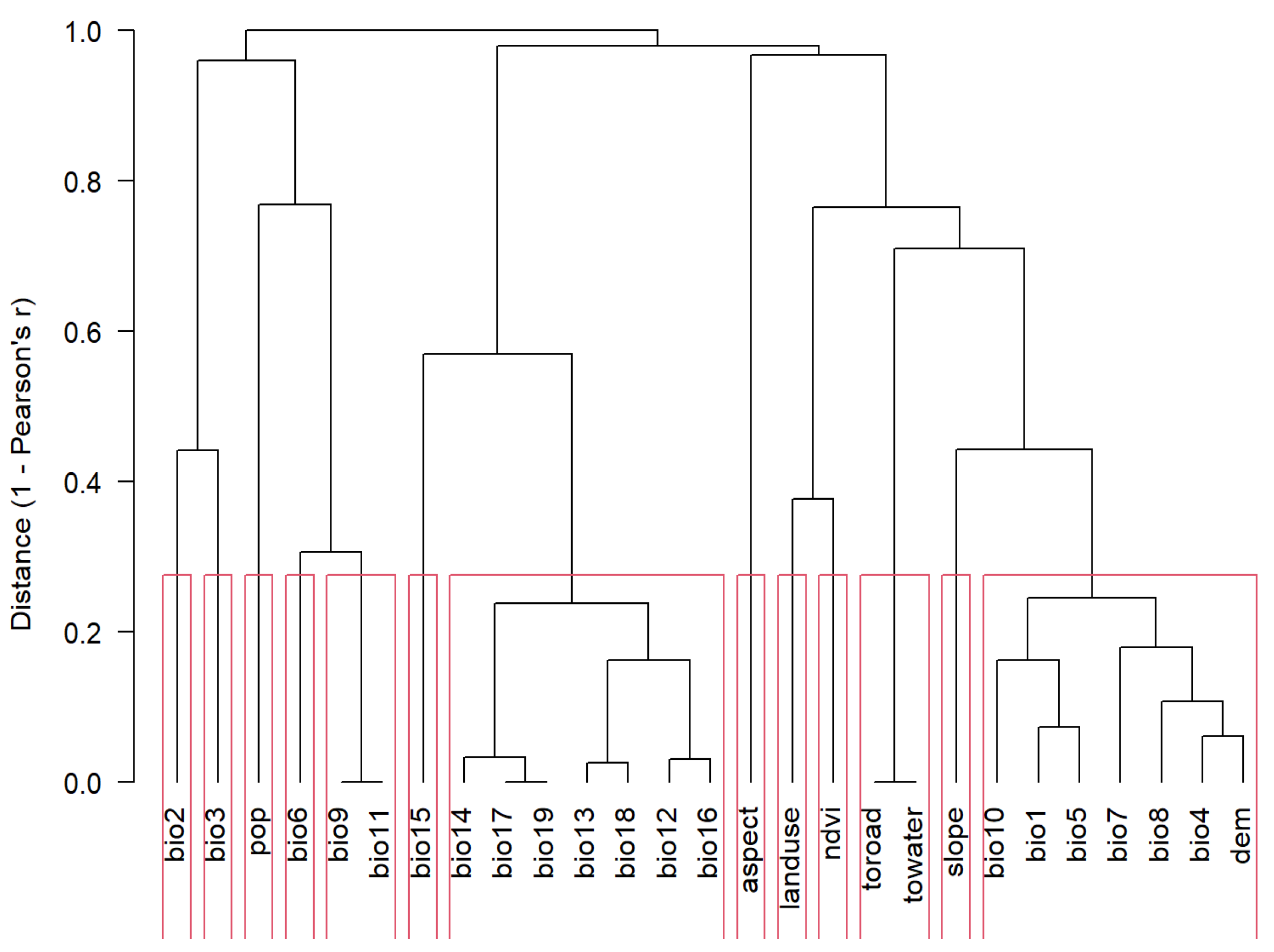
3.1. Environment Variable Filtering Results

Among the groups of variables with correlation coefficients greater than 0.7 in Figure 2, we selected only the group with the greatest contribution to participate in the MaxEnt model and, finally, selected 12 variables each for wetland plants and waterfowl to participate in the model predictions (Table 2).

3.2. Model Performance Assessment

According to the prediction results simulated by the MaxEnt model, the AUC values for the training set of the ROC curves for wetland plants and waterfowl were 0.821 and 0.811, respectively, and the AUC values for the test level were 0.820 and 0.853, respectively. Indicating that the simulation of the geographic distribution of predicted species in Zhengzhou City by using the MaxEnt model was accurate. The obtained curves are shown in Figure 3.

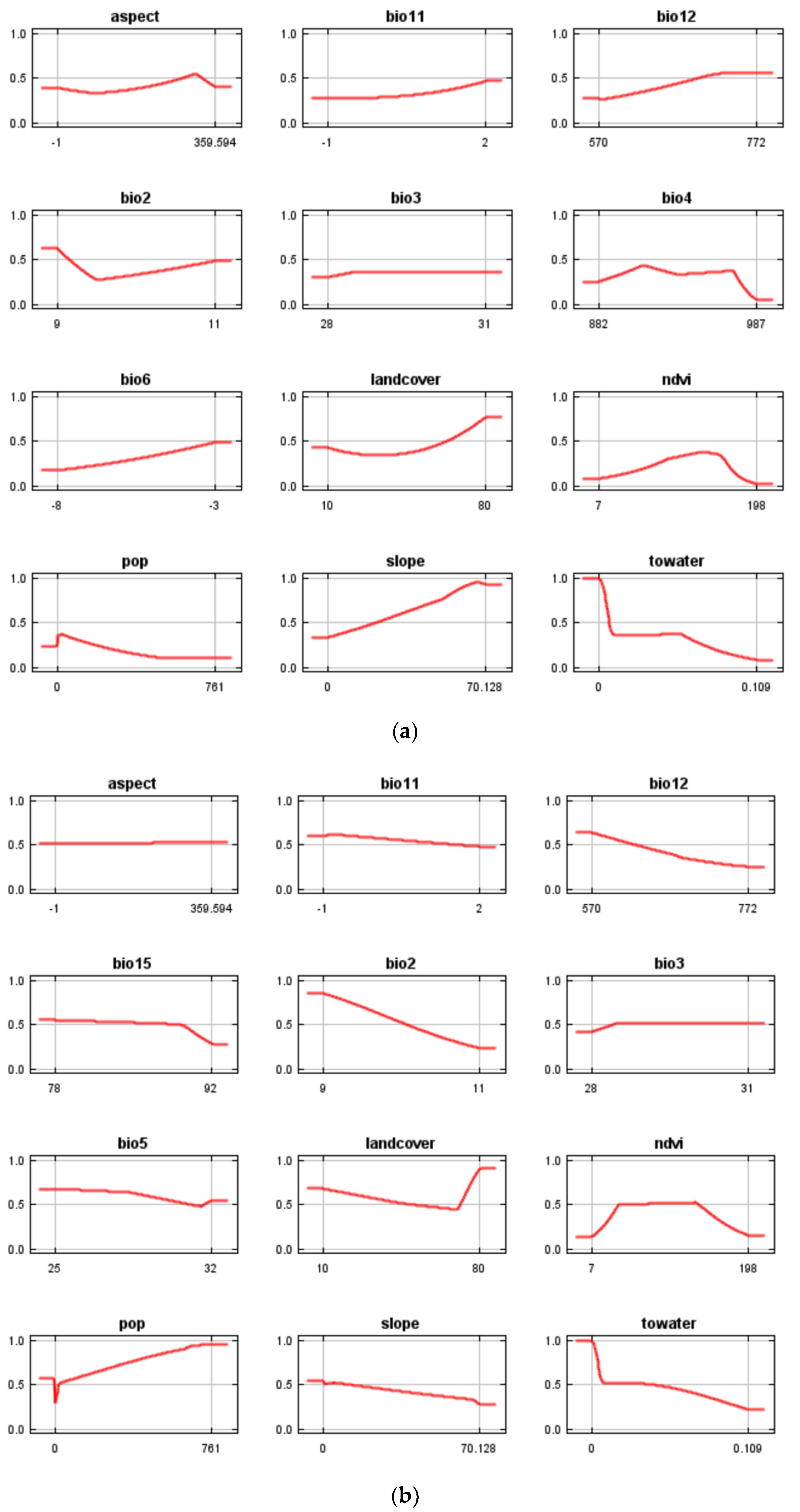
3.3. Elements Influencing the Potential Geographic Distribution of Species

Of the 12 environmental factor variables used for MaxEnt model prediction, the following table shows the estimated relative contribution (Percent contribution) of the environmental variables to the MaxEnt model. The top three environmental variables contributing to the potential geographic distribution of wetland plants were, in order, distance to water bodies (to water, 56.3%), seasonal variation in precipitation (BIO15, 16%), and the normalized vegetation index (NDVI, 5.6%). The top three environmental variables contributing to the potential geographic distribution of waterfowl were: distance to water bodies (to water, 64%), population density (POP, 12.3%), and daily difference in the mean temperature (BIO2, 7.4%).

Permutation importance is the value that randomly displaces each environmental factor on the training presence and background data, with larger values indicating a stronger model dependence on that variable. Permutation importance values of environmental factors affecting the potential geographic distribution of various species are shown in

Table 3. Analysis of the variable contributions.

Wetland Species	Percent Contribution	Permutation Importance
Wetland plants	Distance to water, 56.3%	Distance to water, 44.1%
	BIO15, 16%	BIO4, 13.5%
	NDVI, 5.6%	NDVI, 9.3%
	BIO12, 3.6%	Landcover, 8%
	Landcover, 3.6%	BIO2, 5.7%
	Population density, 3.6%	Slope, 5.5%
	Aspect, 3.3%	BIO11, 4.3%
	BIO11, 2.6%	BIO12, 4%
	Slope, 2.3%	Aspect, 2.4%
	BIO2, 2.2%	Population density, 1.4%
	BIO3, 0.5%	BIO3, 1%
	BIO6, 0.3%	BIO6, 0.7%
Waterfowl	Distance to water, 64%	Distance to water, 49.5%
	Population density, 12.3%	Population density, 12.3%
	BIO2, 7.4%	BIO2, 9.5%
	Landcover, 5.8%	Landcover, 7.6%
	NDVI, 4.9%	Slope, 6.6%
	Slope, 2.3%	NDVI, 6.2%
	BIO15, 0.8%	BIO11, 3.8%
	BIO5, 0.7%	BIO3, 3%
	BIO12, 0.5%	Aspect, 1.4%
	Aspect, 0.5%	BIO12, 0.1%
	BIO3, 0.4%	BIO15, 0%
	BIO11, 0.4%	BIO5, 0%

The biological variables are explained in detail in Table 1.

. Response curves show how each variable affects the MaxEnt prediction (Figure A2).

It can be seen from Figure 4 that, when only a single environmental factor variable is used, the three environmental factor variables with the highest regularized training gain for wetland plants are: distance to water body (to water, 0.284), land cover (0.0613), and temperature seasonality (BIO4, 0.054). The three environmental variables with the most significant gain in waterfowl regularization training were: distance from the water body (to water, 0.4012), land cover (land cover, 0.1444), and population density (pop, 0.1329). As for the results of the “In addition to this variable” score, the factors with the smallest gain for wetland plants were distance from water bodies (to water, 0.288), landcover (0.5538), and temperature seasonality (BIO, 0.5574). The factors with the smallest gain for waterfowl were distance to water body (to water, 0.4534), population density (pop, 0.5819), and land cover (0.5841).

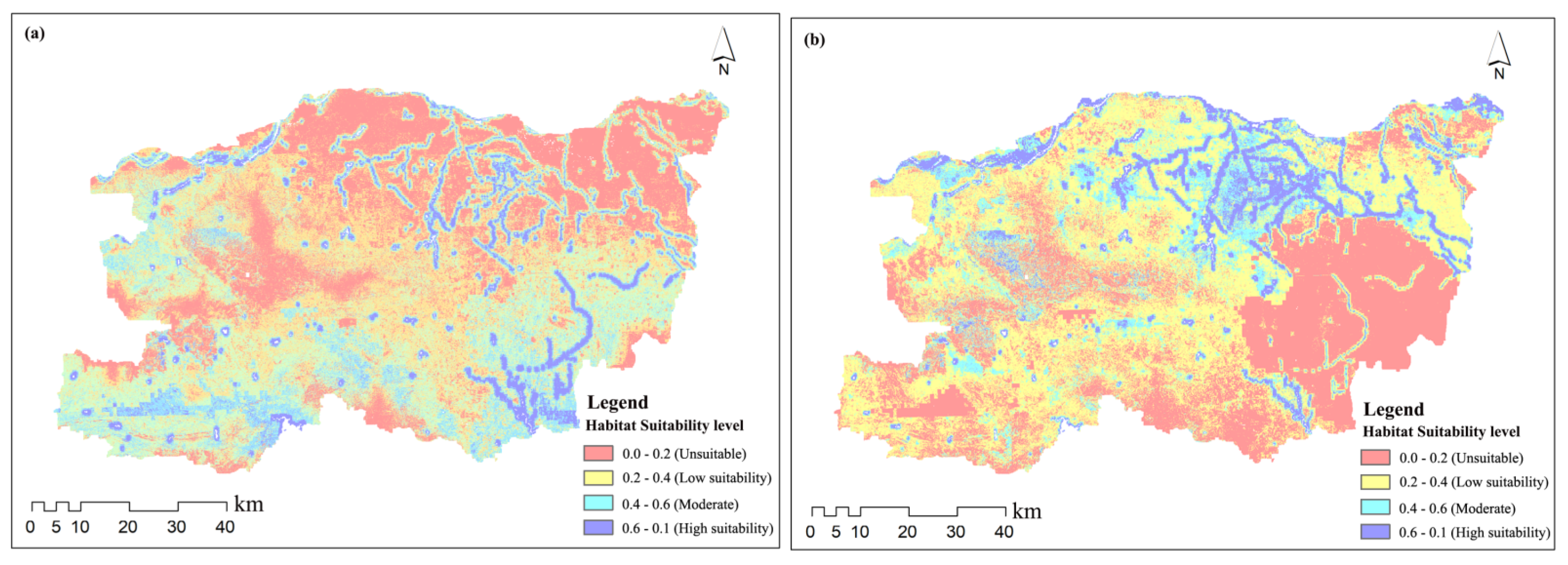
3.4. Identification of Potential Geographic Habitats of Species

The final habitat suitability map of wetland species in Zhengzhou City is shown in Figure 5. Using ArcGIS 10.8 to calculate the area of the distribution raster data, high suitability habitat areas for wetland plants and waterfowl were obtained as 78,613.84 ha and 71,129.79 ha, respectively. They account for 10.56% and 9.55% of the total area of Zhengzhou City, respectively. The unsuitable areas were 226,579.86 ha and 248,153 ha, accounting for 30.43% and 33.33% of the total area of Zhengzhou City, respectively. Influenced by the distribution of the wetlands, the best potential geographic distribution areas of wetland plants in Zhengzhou are found in the northern and southeastern regions of the city, while the best potential geographic distribution areas of waterfowl are concentrated in the densely distributed areas of water systems in the northern part of the city.

4. Discussion

4.1. Validity of the Model

Although the number and area covered by protected areas continue to grow globally, it does not mean that these protected areas cover the full range of species [44]. Especially in rapidly urbanizing areas, the dramatic increase in gray infrastructure has disrupted the original ecosystem balance and affected wetlands such as rivers and lakes in cities [45]. Based on the MaxEnt model, this paper uses species distribution point data and environmental variables, including bioclimatic, topography, land cover, population density, and distance to road water bodies, to predict the current potential suitable range of wetland plants and waterfowl in Zhengzhou City and to make a preliminary assessment of the effectiveness of wetland species conservation in existing protected areas (PA). The model prediction results were verified by ROC curve accuracy, and the model prediction results were good. The main findings are described in the following subsections.

4.2. Variables Contribution and Similarities and Differences with Other Studies

The geographic distribution of wetland species is mainly governed by water body distribution, bioclimatic, and population density. In terms of percent contribution, the factor that contributed most to the distribution of wetland plants and waterbirds during this period was distance to a water body. The second-most important factors were seasonal variation in precipitation and population density, respectively. This is also in general agreement with Karen A. Poiani et al. [46] that seasonal variations in precipitation affect the hydrology and vegetation of wetlands. Wetland plants and waterfowl, as species closely associated with freshwater habitats, are important indicators of ecosystem health [47]. Land use changes have reduced the habitat availability at waterfowl stopovers and overwintering sites [48]. As urban water bodies exhibit highly variable morphological characteristics [49], urbanization reduces or alters aquatic habitat for waterfowl using water for municipal purposes, in turn creating habitats from built infrastructures or altering existing streams, rambling beaches, or wetlands [50]. During the construction of new urban areas over the past 20 years, several new lakes have been built in Zhengzhou City [27], and these new wetland water bodies have become an increasingly active area for birds [51]. The use of artificial wetlands by wildlife also confirms that the construction of artificial wetlands may offset the negative impacts of urbanization on biodiversity to some extent [52,53], but localized increases in water area are not the norm in most cities [54].

4.3. Implications of the Study Results for Conservation Planning

High suitability habitat areas for various wetland species in Zhengzhou are 78,613.84 ha for plants and 71,129.79 ha for waterfowl. At present, the only nature reserve in Zhengzhou, Zhengzhou Yellow River Wetland Nature Reserve, covers only 8061.3 ha of wetland plants and 12,472.9 ha of waterfowl, which are 10.25% and 17.54% of the total area of the high suitability habitat for species in the whole area of Zhengzhou. Therefore, there are still a lot of gaps in the habitat of species outside the protected areas that need to be protected and managed. For other wetland species hotspot areas that are not included in PAs, various forms of protection can be adopted based on existing policies. For example, in the year 2004, the General Office of the State Council mentioned in the “Notice on Strengthening Wetland Protection and Management”: for areas that do not have the conditions for designating nature reserves, they can establish small wetland PAs, wetland parks, wetland multifunctional management areas, or designate wildlife habitats in accordance with local conditions to strengthen their protection and management [55]. In fact, the importance of small wetlands for the persistence of local wetland-associated animal populations was demonstrated in studies as early as 1993 [56]. Although some species have shown adaptability to urbanization [57], methods for creating natural habitats in the city and maximizing the protection of habitats suitable for wetland species still need to be explored in future research.

4.4. Limitations

Although this study incorporated environmental factors such as topography, land cover, habitat suitability, and population density into the prediction of wetland species’ fitness zones, some ecological niches are difficult to represent by environmental factors. The relationships within species and between populations also limit species dispersal, and their distribution changes to some extent, which is challenging to incorporate into the model. Therefore, they may bring some bias to predicting species’ fitness zones. In the future, other factors can be considered comprehensively. The most direct environmental factors affecting species distribution can be selected as far as possible to make the prediction results more accurate.

5. Conclusions

Species distribution modeling is becoming increasingly important in habitat research, not only to determine the environmental needs of species scientifically but also to provide strong support for subsequent habitat conservation. In this paper, the MaxEnt model was used to identify the potential geographic distribution range and conservation gaps of wetland species in Zhengzhou City. At present, the existing protected areas in Zhengzhou cover no more than 20% of the high suitability area of wetland species in Zhengzhou. The existing protected areas in Zhengzhou City are not sufficient to protect the integrity of the potential geographic distribution areas of wetland species in Zhengzhou City. For the hotspots of wetland species distribution that are not included in the protected areas, we can take the establishment of small wetland reserves, wetland parks, and other forms of protection and management according to local conditions.

References

1. Ma, Z.; Li, B.; Zhao, B.; Jing, K.; Tang, S.; Chen, J. Are Artificial Wetlands Good Alternatives to Natural Wetlands for Waterbirds?—A Case Study on Chongming Island, China. Biodivers. Conserv. 2004, 13, 333–350. [Google Scholar] [CrossRef]
2. Murray, C.G.; Kasel, S.; Loyn, R.H.; Hepworth, G.; Hamilton, A.J. Waterbird Use of Artificial Wetlands in an Australian Urban Landscape. Hydrobiologia 2013, 716, 131–146. [Google Scholar] [CrossRef]
3. Rodríguez-Rodríguez, D.; Rodríguez-Rodríguez, D. New Issues on Protected Area Management; IntechOpen: London, UK, 2012; ISBN 978-953-51-0697-5. [Google Scholar]
4. Guo, Z.; Cui, G.; Zhang, M.; Li, X. Analysis of the Contribution to Conservation and Effectiveness of the Wetland Reserve Network in China Based on Wildlife Diversity. Glob. Ecol. Conserv. 2019, 20, e00684. [Google Scholar] [CrossRef]
5. Hostetler, M.; Knowles-Yanez, K. Land Use, Scale, and Bird Distributions in the Phoenix Metropolitan Area. Landsc. Urban Plan. 2003, 62, 55–68. [Google Scholar] [CrossRef]
6. Ferrier, S. Mapping Spatial Pattern in Biodiversity for Regional Conservation Planning: Where to from Here? Syst. Biol. 2002, 51, 331–363. [Google Scholar] [CrossRef]
7. Erickson, K.D.; Smith, A.B. Accounting for Imperfect Detection in Data from Museums and Herbaria When Modeling Species Distributions: Combining and Contrasting Data-Level versus Model-Level Bias Correction. Ecography 2021, 44, 1341–1352. [Google Scholar] [CrossRef]
8. Rodrigues, A.S.L.; Gregory, R.D.; Gaston, K.J. Robustness of Reserve Selection Procedures under Temporal Species Turnover. Proc. R. Soc. London. Ser. B Biol. Sci. 2000, 267, 49–55. [Google Scholar] [CrossRef] [Green Version]
9. Pressey, R.L. Conservation Planning and Biodiversity: Assembling the Best Data for the Job. Conserv. Biol. 2004, 18, 1677–1681. [Google Scholar] [CrossRef]
10. Cayuela, L.; Golicher, D.J.; Newton, A.C.; Kolb, M.; de Alburquerque, F.S.; Arets, E.J.M.M.; Alkemade, J.R.M.; Pérez, A.M. Species Distribution Modeling in the Tropics: Problems, Potentialities, and the Role of Biological Data for Effective Species Conservation. Trop. Conserv. Sci. 2009, 2, 319–352. [Google Scholar] [CrossRef] [Green Version]
11. Gogol-Prokurat, M. Predicting Habitat Suitability for Rare Plants at Local Spatial Scales Using a Species Distribution Model. Ecol. Appl. 2011, 21, 33–47. [Google Scholar] [CrossRef]
12. Franklin, J.; Miller, J.A. Mapping Species Distributions: Spatial Inference and Prediction; Cambridge University Press: Cambridge, UK, 2010; ISBN 978-0-521-87635-3. [Google Scholar]
13. Ottaviani, D.; Lasinio, G.J.; Boitani, L. Two Statistical Methods to Validate Habitat Suitability Models Using Presence-Only Data. Ecol. Model. 2004, 179, 417–443. [Google Scholar] [CrossRef]
14. Booth, T.H.; Nix, H.A.; Busby, J.R.; Hutchinson, M.F. Bioclim: The First Species Distribution Modelling Package, Its Early Applications and Relevance to Most Current MaxEnt Studies. Divers. Distrib. 2014, 20, 1–9. [Google Scholar] [CrossRef]
15. Hirzel, A.H.; Arlettaz, R. Modeling Habitat Suitability for Complex Species Distributions by Environmental-Distance Geometric Mean. Environ. Manag. 2003, 32, 614–623. [Google Scholar] [CrossRef] [Green Version]
16. Busby, J.R. A Biogeoclimatic Analysis of Nothofagus Cunninghamii (Hook.) Oerst. in Southeastern Australia. Aust. J. Ecol. 1986, 11, 1–7. [Google Scholar] [CrossRef]
17. Carpenter, G.; Gillison, A.N.; Winter, J. DOMAIN: A Flexible Modelling Procedure for Mapping Potential Distributions of Plants and Animals. Biodivers. Conserv. 1993, 2, 667–680. [Google Scholar] [CrossRef]
18. Elith, J.; Leathwick, J.R. Spccies Distribution Models: Ecological Explanation AndPrediction Across Space and Time. Spccies Distrib. Model. Ecol. Explan. Across Space Time 2009, 40, 677–697. [Google Scholar] [CrossRef]
19. Zhang, L. Application of MAXENT maximum entropy model in predicting the potential distribution range of species. Ecol. Bull. 2015, 50, 9–12. [Google Scholar]
20. Wisz, M.S.; Hijmans, R.J.; Li, J.; Peterson, A.T.; Graham, C.H.; Guisan, A.; NCEAS Predicting Species Distributions Working Group. Effects of Sample Size on the Performance of Species Distribution Models. Divers. Distrib. 2008, 14, 763–773. [Google Scholar] [CrossRef]
21. Hernandez, P.A.; Graham, C.H.; Master, L.L.; Albert, D.L. The Effect of Sample Size and Species Characteristics on Performance of Different Species Distribution Modeling Methods. Ecography 2006, 29, 773–785. [Google Scholar] [CrossRef]
22. Ortega-Huerta, M.A.; Townsend Peterson, A. Modeling Ecological Niches and Predicting Geographic Distributions: A Test of Six Presence-Only Methods. Rev. Mex. Biodivers. 2008, 79, 205–216. [Google Scholar]
23. Phillips, S.J.; Anderson, R.P.; Schapire, R.E. Maximum Entropy Modeling of Species Geographic Distributions. Ecol. Model. 2006, 190, 231–259. [Google Scholar] [CrossRef] [Green Version]
24. Kong, X. Stability Assessment of Species Distribution Models and Application Software. Master’s Thesis, Anqing Normal University, Anqing, China, 2015. [Google Scholar]
25. Keller, D.; Holderegger, R.; van Strien, M.J.; Bolliger, J. How to Make Landscape Genetics Beneficial for Conservation Management? Conserv. Genet. 2015, 16, 503–512. [Google Scholar] [CrossRef]
26. Tulloch, A.I.T.; Sutcliffe, P.; Naujokaitis-Lewis, I.; Tingley, R.; Brotons, L.; Ferraz, K.M.P.M.B.; Possingham, H.; Guisan, A.; Rhodes, J.R. Conservation Planners Tend to Ignore Improved Accuracy of Modelled Species Distributions to Focus on Multiple Threats and Ecological Processes. Biol. Conserv. 2016, 199, 157–171. [Google Scholar] [CrossRef] [Green Version]
27. Xue, C.Q.L.; Wang, Y.; Tsai, L. Building New Towns in China–A Case Study of Zhengdong New District. Cities 2013, 30, 223–232. [Google Scholar] [CrossRef]
28. Wang, X.; Tomaney, J. Zhengzhou–Political Economy of an Emerging Chinese Megacity. Cities 2019, 84, 104–111. [Google Scholar] [CrossRef]
29. Brown, J.L.; Bennett, J.R.; French, C.M. SDMtoolbox 2.0: The next Generation Python-Based GIS Toolkit for Landscape Genetic, Biogeographic and Species Distribution Model Analyses. PeerJ 2017, 5, e4095. [Google Scholar] [CrossRef] [Green Version]
30. Hijmans, R.J. Cross-Validation of Species Distribution Models: Removing Spatial Sorting Bias and Calibration with a Null Model. Ecology 2012, 93, 679–688. [Google Scholar] [CrossRef] [Green Version]
31. Fick, S.E.; Hijmans, R.J. WorldClim 2: New 1-Km Spatial Resolution Climate Surfaces for Global Land Areas. Int. J. Climatol. 2017, 37, 4302–4315. [Google Scholar] [CrossRef]
32. Zanaga, D.; Van De Kerchove, R.; De Keersmaecker, W.; Souverijns, N.; Brockmann, C.; Quast, R.; Wevers, J.; Grosu, A.; Paccini, A.; Vergnaud, S.; et al. ESA WorldCover 10 m 2020 V100 2021. Available online: https://zenodo.org/record/5571936 (accessed on 26 August 2021).
33. Gregorio, A.D.; Jansen, L.J.M.; Food and Agriculture Organization of the United Nations. Land Cover Classification System: Classification Concepts and User Manual: LCCS; Food & Agriculture Organization: Rome, Italy, 2005; ISBN 978-92-5-105327-0. [Google Scholar]
34. Vermote, E.; Justice, C.; Claverie, M.; Franch, B. Preliminary Analysis of the Performance of the Landsat 8/OLI Land Surface Reflectance Product. Remote Sens. Environ. 2016, 185, 46–56. [Google Scholar] [CrossRef]
35. Warren, D.L.; Matzke, N.J.; Cardillo, M.; Baumgartner, J.B.; Beaumont, L.J.; Turelli, M.; Glor, R.E.; Huron, N.A.; Simões, M.; Iglesias, T.L.; et al. ENMTools 1.0: An R Package for Comparative Ecological Biogeography. Ecography 2021, 44, 504–511. [Google Scholar] [CrossRef]
36. Leroy, B.; Meynard, C.N.; Bellard, C.; Courchamp, F. Virtualspecies, an R Package to Generate Virtual Species Distributions. Ecography 2016, 39, 599–607. [Google Scholar] [CrossRef] [Green Version]
37. Yang, X.-Q.; Kushwaha, S.P.S.; Saran, S.; Xu, J.; Roy, P.S. Maxent Modeling for Predicting the Potential Distribution of Medicinal Plant, Justicia Adhatoda L. in Lesser Himalayan Foothills. Ecol. Eng. 2013, 51, 83–87. [Google Scholar] [CrossRef]
38. Kong, W.; Li, X. Optimization of maximum entropy models in species distribution prediction. J. Appl. Ecol. 2019, 30, 2116. [Google Scholar] [CrossRef]
39. Zhang, H.; Zhao, H.; Xu, C. The potential geographical distribution of Alsophila spinulosain under climate change in China. Chin. J. Ecol. 2021, 40, 968–979. [Google Scholar] [CrossRef]
40. Zhang, H.; Zhao, H.; Wang, H. Potential Geographical Distribution of Populus Euphratica in China under Future Climate Change Scenarios Based on Maxent Model. Acta Ecol. Sin. 2020, 40, 6552–6563. [Google Scholar] [CrossRef]
41. Ning, Y.; Jin, R. Modeling the potential suitable habitat of Impatiens hainanensis, a limestone-endemic plant. J. Plant Ecol. 2018, 42, 946. [Google Scholar] [CrossRef] [Green Version]
42. Swets, J.A. Measuring the Accuracy of Diagnostic Systems. Science 1988, 240, 1285–1293. [Google Scholar] [CrossRef] [Green Version]
43. Yusup, S.; Sulayman, M.; Ilghar, W. Prediction of Potential Distribution of Didymodon (Bryophyta, Pottiaceae) in Xinjiang Based on the MaxEnt Model. Plant Sci. J. 2018, 36, 541–553. [Google Scholar] [CrossRef]
44. Rodríguez-Rodríguez, D.; Martínez-Vega, J. Proposal of a System for the Integrated and Comparative Assessment of Protected Areas. Ecol. Indic. 2012, 23, 566–572. [Google Scholar] [CrossRef] [Green Version]
45. Wang, H.; Huang, L.; Hu, J.; Yang, H.; Guo, W. Effect of Urbanization on the River Network Structure in Zhengzhou City, China. Int. J. Environ. Res. Public Health 2022, 19, 2464. [Google Scholar] [CrossRef]
46. Poiani, K.A.; Johnson, W.C.; Kittel, T.G.F. Sensitivity of a Prairie Wetland to Increased Temperature and Seasonal Precipitation Changes1. JAWRA J. Am. Water Resour. Assoc. 1995, 31, 283–294. [Google Scholar] [CrossRef]
47. Ogden, J.C.; Baldwin, J.D.; Bass, O.L.; Browder, J.A.; Cook, M.I.; Frederick, P.C.; Frezza, P.E.; Galvez, R.A.; Hodgson, A.B.; Meyer, K.D.; et al. Waterbirds as Indicators of Ecosystem Health in the Coastal Marine Habitats of Southern Florida: 1. Selection and Justification for a Suite of Indicator Species. Ecol. Indic. 2014, 44, 148–163. [Google Scholar] [CrossRef]
48. Shorebirds in Western North America: Late 1800s to Late 1900s. Available online: https://pubs.er.usgs.gov/publication/70185084 (accessed on 10 March 2022).
49. Waterbird Populations Estimates, 5th ed; Mundkur, T.; Nagy, S. (Eds.) Wetlands International: Wageningen, The Netherlands, 2012. [Google Scholar]
50. Grimm, N.B.; Faeth, S.H.; Golubiewski, N.E.; Redman, C.L.; Wu, J.; Bai, X.; Briggs, J.M. Global Change and the Ecology of Cities. Science 2008, 319, 756–760. [Google Scholar] [CrossRef] [PubMed] [Green Version]
51. Liu, C.; Minor, E.S.; Garfinkel, M.B.; Mu, B.; Tian, G. Anthropogenic and Climatic Factors Differentially Affect Waterbody Area and Connectivity in an Urbanizing Landscape: A Case Study in Zhengzhou, China. Land 2021, 10, 1070. [Google Scholar] [CrossRef]
52. De Martis, G.; Mulas, B.; Malavasi, V.; Marignani, M. Can Artificial Ecosystems Enhance Local Biodiversity? The Case of a Constructed Wetland in a Mediterranean Urban Context. Environ. Manag. 2016, 57, 1088–1097. [Google Scholar] [CrossRef] [Green Version]
53. Giosa, E.; Mammides, C.; Zotos, S. The Importance of Artificial Wetlands for Birds: A Case Study from Cyprus. PLoS ONE 2018, 13, e0197286. [Google Scholar] [CrossRef] [Green Version]
54. Xie, C.; Huang, X.; Wang, L.; Fang, X.; Liao, W. Spatiotemporal Change Patterns of Urban Lakes in China’s Major Cities between 1990 and 2015. Int. J. Digit. Earth 2018, 11, 1085–1102. [Google Scholar] [CrossRef]
55. General Office of the State Council on Strengthening the Protection and Management of Wetlands Notice. Available online: http://www.gov.cn/zwgk/2005-08/15/content_22930.htm (accessed on 28 August 2022).
56. Gibbs, J.P. Importance of Small Wetlands for the Persistence of Local Populations of Wetland-Associated Animals. Wetlands 1993, 13, 25–31. [Google Scholar] [CrossRef]
57. Shui-Hua, C.; Ping, D.; Yang, Z. Impacts of Urbanization on the Wetland Waterbird Communities in Hangzhou. Zool. Res. 2000, 21, 279–285. [Google Scholar]
Figure 1. (a) Location of Zhengzhou, Henan Province, in China; gray lines indicate the boundaries of provinces and territories. (b) Henan Province; black lines depict city boundaries. (c) The blue line shows the boundary of Zhengzhou City, which can be seen to the north of Zhengzhou close to the Yellow River, the second-longest river in China.
Land 12 00221 g001
Figure 2. Groups of intercorrelated variables at a cut-off of 0.7.
Land 12 00221 g002
Figure 3. AUC values of ROC curves for (a) wetland plants and (b) waterfowl.
Land 12 00221 g003
Figure 4. The jackknife test result of environment factor for (a) wetland plants and (b) waterfowl.
Land 12 00221 g004
Figure 5. Classification of (a) the wetland plants and (b) waterfowl habitat suitability levels in Zhengzhou.
Land 12 00221 g005