Relationship between Land-Use Type and Daily Concentration and Variability of PM10 in Metropolitan Cities: Evidence from South Korea

Abstract

Since urban areas with high air pollution are known to have higher mortality rates compared to areas with less air pollution, accurately understanding and predicting the distribution of particulate matter (PM) in cities is important for urban planning policies that seek to emphasize the health of citizens. Therefore, this study aims to investigate the relationship between PM and land use in metropolitan cities in South Korea using the land-use regression model. We use daily data from the air quality monitoring stations (AQMS) in seven cities in South Korea for the year 2018. For analysis, K-means clustering is employed to identify the land-use pattern surrounding the AQMSs and two log-lin regression models are used to investigate the effects of each land-use type on PM. The findings show a statistically significant difference in PM concentration and variability in the business, commercial, industrial, mixed, and high-density residential areas compared to parks and green areas, and that PM concentration and variability were less in mixed areas than in single land use, thus verifying the effectiveness of a mixed land-use planning strategy. Moreover, microclimatic, seasonal, and regional factors affect PM concentration and variability. Finally, to minimize exposure to PM, various policies such as mixed land use need to be established and implemented differently, depending on the season and time.

1. Introduction

Particulate matter (PM), along with ozone (O₃) and nitrogen dioxide (NO₂), is one of the most significant air pollutants that threaten the health of humans worldwide. PM is widely considered as an air pollutant with a large impact on health [1,2]. It is classified according to the particle diameter, and particles with a diameter of 10 μm or less are called PM10. PM2.5, which has a particle diameter of less than 2.5 μm, is attracting attention, but many studies have reported that the particle size causes different health outcomes through different biological mechanisms [2]. Therefore, PM10 still needs to be studied separately from PM2.5.

The main sources of PM are traffic, industry, domestic fuel burning (including cooking, heating, etc.), natural sources (including soil dust and sea salt), and unspecified sources of human origin [3]. Globally, the contribution of natural sources to PM10 is 22% [3], in other words 78% of PM10 originates from human activities. The contribution of sources related to human activity is traffic (25%), industry (18%), domestic fuel burning (15%), and unspecified sources of human origin (20%) [3]. The contribution of natural sources in Korea is 16% [3], which is lower than the global average, and, therefore, it is a country where human activities have a large influence on PM10 concentration.

The OECD predicts that by 2060, there will be 1109 premature deaths per million people in South Korea due to air pollution if no additional policy measures are implemented; furthermore, the economic damage from air pollution is expected to be the largest among OECD countries [4]. In 2016, the annual mean PM10 level in Seoul (46 µg/m³) was much higher than that in cities such as Los Angeles (19 µg/m³), New York (16 µg/m³), Paris (27 µg/m³), and London (19 µg/m³) [5]. In other words, the PM situation in South Korea is very serious, and the damage to public health and the economy is expected to be significant.

Specifically, local background concentration is an important indicator of quality management in air environments [6]. Therefore, to adequately respond to the risk of PM exposure, it is necessary to properly predict the PM concentration and prepare countermeasures. Studies analyzing the variability of air pollutants by region have historically focused on inter-city variability [7]. However, the magnitude of intra-city PM variability is not small compared to inter-city PM variability; indeed, in some cases, it is greater [8]. The difference in PM concentration within a city is closely related to the spatial distribution of local PM sources, such as transportation, cooking, and biomass burning [9,10]. In particular, the relationship between traffic and PM concentration has been intensively studied [11,12].

Additionally, the spatial variability of PM concentrations in cities is related to regional health [13,14]. Therefore, accurately understanding and predicting the distribution of PM in cities is important for various urban policies and for the health of citizens.

The best way to understand and predict spatial differences in PM concentrations in a city is by installing a sufficient number of PM monitoring stations and collecting data continuously. However, there is a financial limit to the implementation of this policy. In particular, in developing countries, where the damage caused by PM is severe, the limitations are starker. Consequently, owing to the lack of monitoring stations, difficulties often arise in the development of models that can accurately predict PM concentrations over large areas [15].

To overcome the problem of insufficient monitoring station data, the first approach is to spatially interpolate the measurement values of the monitoring stations using methods such as inverse distance weighting (IDW) and kriging [16,17,18,19,20]. However, the interpolation approach has low accuracy, as it uses only the geographic distance between monitoring stations [21,22]. The variability of PM concentration in a city is influenced by the complex spatial composition of the city, created by the cumulative changes in land use [23]. Additionally, dense buildings impede the dispersion of PM in high-density cities [24], contributing to the spatial differences in PM concentrations. Accordingly, the morphological factors of cities and buildings also affect spatial differences in PM.

Another approach to overcome the limitations of insufficient monitoring station data is the land-use regression (LUR) model, which estimates the concentration of pollutants, such as PM, by region by considering the impact of land use in the city. The LUR model is a robust multiple regression technique that uses explanatory variables, such as traffic, land use, physical environment, and population density to predict the concentration of air pollutants in a target area as measured at the monitoring station (i.e., the dependent variable) [18,25,26,27]. Initially, it was applied in Europe [25,28,29]; however, it has recently been used in other regions, including North America [30,31,32,33] and Asia [6,15,22,34,35,36,37].

There is no standard way to build an LUR model, as various approaches have been employed [27]. In general, the pollutant concentration is used as the dependent variable, whereas the land-use environment surrounding the monitoring station is the main explanatory variable. To measure the contaminant concentration as a dependent variable, it is ideal to select a location of the monitoring station that can optimize the spatial variability; however, many studies utilize data from the existing monitoring station network [30,35,38]. Land use, population density, point pollution sources, and traffic patterns are mainly used as explanatory variables representing the land-use environment around the monitoring station [15,34]. Furthermore, meteorological variables, such as precipitation, wind speed, wind direction, and temperature, are often used as explanatory variables [6,36,39].

Although land-use environment variables, such as land use, population density, and traffic volume have large spatial variability, they show small temporal variability at the same location. In contrast, meteorological variables have small spatial variability within a city but large temporal variability. Therefore, land-use environment variables can be considered variables that explain spatial variability, and meteorological variables can be regarded as variables that explain temporal variability [21]. That is, the use of detailed land-use environment and microscopic meteorological variables increases the spatial and temporal resolution of the LUR model, respectively. Precisely quantifying the temporal and spatial variability of air pollution can provide a more accurate pollutant exposure assessment [40].

Subsequently, the LUR model was refined, and various variables were added in the course of its development. However, most studies using the LUR model focused on modeling the spatial variability of air pollution, whereas the temporal variability was mostly treated as an average [15]. Therefore, the spatial resolution of the pollutant distribution in a city has increased with the development of the LUR model, whereas the temporal resolution remains relatively low.

Although research to increase the temporal resolution of LUR models has been conducted in recent years, most LUR model studies have focused on annual or seasonal average concentrations with low temporal resolution [21]. In particular, most LUR models are based on annual average data [26], which may be sufficient to study the damage caused by long-term exposure; however, the temporal resolution is insufficient to study the damage caused by short- and medium-term exposure [21].

Temporal variability in PM concentrations is very large in South Korea. In 2018, the average, maximum, and minimum PM10 hourly values of the monitoring station in Jung-gu, Seoul were 36.2, 296, and 3, respectively, with a standard deviation of 24.1. Additionally, the mean, maximum, minimum PM2.5 hourly values were 21.5, 132, and 1, respectively, with a standard deviation of 16.0 [41]. This variability is related to the climatic characteristics of the Korean Peninsula, where the yellow dust phenomenon occurs from winter to spring. It originates in the deserts of China, Mongolia, and Kazakhstan [42] located to the west of the Korean Peninsula. In the Korean Peninsula, the northwest wind blows mainly in the winter season, affected by the Siberian air mass [43], while the southeast wind blows mainly in the summer season, affected by the North Pacific air mass [44]. Therefore, the yellow dust phenomenon appears from winter to spring when the western wind is strong. Consequently, the PM concentration is high in winter and spring. Before the high PM10 episode in Korea, the movement of aerosols from China to the Korean Peninsula was confirmed through satellite imagery [45]. China contributes 32.1% to the PM2.5 concentrations in Korea [46].

However, most studies dealing with LUR models in Korea have focused on increasing the spatial resolution. Furthermore, although studies have been conducted to increase spatial resolution using machine learning [47] and the geographically weighted regression model (GWR) [48], only the average annual pollution concentration and average annual meteorological variables are still being used.

Another limitation in the process of estimating PM concentration using LUR in Korea is the location of the monitoring stations, which is an important factor influencing the measurement of PM concentrations in cities [49]. PM monitoring stations in South Korea are distributed based on administrative districts rather than spatial characteristics. Additionally, in terms of ease of installation and management, they are mainly installed on roofs or gardens of public facilities. Therefore, the location of the monitoring stations is determined by the location of public facilities. Moreover, since the regional characteristic types of monitoring stations are divided into urban, suburban, and roadside in South Korea [41], the environmental characteristics, except for the roadside in the city, are not reflected in the location of the monitoring station.

To overcome these limitations, the present study aims to analyze the relationship between PM and land use in large cities in South Korea using the LUR model. This study contributes to the existing literature in the following ways. First, to increase the temporal resolution, it uses the daily average data, not the annual or monthly averages. Additionally, to better understand the PM temporal variability, we develop a model with daily PM variability as the dependent variable.

Second, instead of directly including land-use environmental variables as independent variables, the land-use environment surrounding the monitoring station is categorized, with the categories used as independent variables. Thereby, it is possible to categorize land use in the area surrounding the current monitoring stations in South Korea and determine the PM distribution according to the location type. This information can help select appropriate locations for PM monitoring stations in the future. Another advantage of categorizing land use is that it can resolve the correlation between land-use-related variables and overcome the limit of reductionism. Land-use environment variables in cities are closely related to each other. For example, in industrial areas, there are many factories that cause pollution, with major roads located nearby and low population density. In such a situation, there is a limit to directly using pollution sources (factories), roads, and population density as independent variables. Reductionism can be divided into three types: ontological, methodological, and theoretical [50]. Among them, methodological reductionism is defined as “the scientific attempt to provide an explanation in terms of ever-smaller entities” [50]. This reductionist approach is not entirely wrong but has limitations. For example, it is not inappropriate to focus on the abilities of players in predicting the performance of a sports team but it has its limitations [51]. Team performance is influenced by coaches, teamwork, facilities, finances, and so on in addition to the players’ capabilities. Therefore, to understand the team’s capabilities, the team, not the players, should be used as the unit of analysis [51]. Thus, to overcome this limitation, studies [52] have categorized and utilized land use. Other studies have removed variables with a high correlation by examining correlations [22].

In this study, two research objectives are considered. First, identifying land-use patterns in the environment surrounding the PM10 measuring stations installed in large cities. The categorization of land use around the measuring station has the advantage of minimizing reductionism errors compared to studies analyzing individual land-use-related variables. Furthermore, if the land use around the measuring station is categorized into neighborhood units, it is possible to present PM10 reduction or adaptive policies based on the analysis results.

Second, examining the relationship between land use in urban areas and the PM10 daily average and variation. Therefore, using the LUR model, this study empirically analyzes the effect of land-use characteristics of neighborhood units on the distribution of PM10 in South Korean urban areas, rather than climatic factors. The land-use characteristics surrounding the PM10 monitoring stations installed in large cities in South Korea are categorized through clustering analysis, and the difference between the daily mean and daily variance of the PM10 concentration for each derived land-use type is empirically verified through the LUR model. Additionally, since human activities in cities are closely related and vary according to land use, by empirically analyzing the effect of land use on the PM10 concentration and variability of PM10, we can derive a spatial planning strategy adaptive to PM10 in urban planning.

2. Materials and Methods

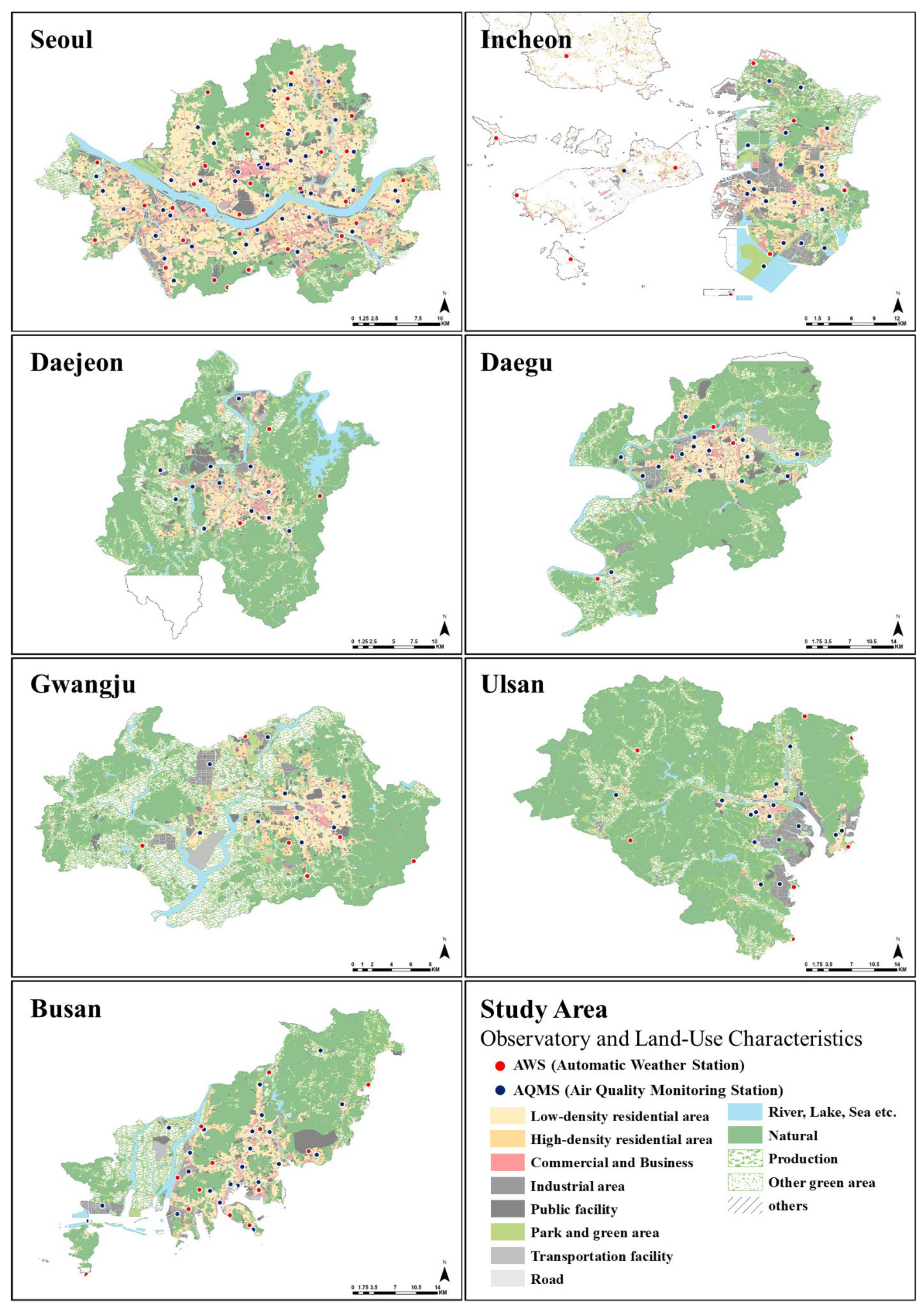
2.1. Scope of Study

This study focuses on PM monitoring stations installed in seven cities in South Korea and the surrounding environment (see Figure 1). With a total population of 51.83 million, about 43% of the population in South Korea lives in metropolitan cities. Based on the Enforcement Decree of the Local Autonomy Act [50], there are mega cities: Seoul (a special metropolitan city,) Busan, Daegu, Incheon, Gwangju, Daejeon, and Ulsan (metropolitan cities.) As of 2020, the populations of Seoul, Busan, Daegu, Incheon, Gwangju, Daejeon, and Ulsan were approximately 9.58, 3.35, 2.41, 2.95, 1.48, 1.49, and 1.14 million, respectively [53].

There are a total of 138 PM measuring stations installed in metropolitan cities in South Korea: 40 in Seoul, 24 in Busan, 20 in Incheon, 17 in Ulsan, 16 in Daegu, 12 in Daejeon, and 9 in Gwangju [41]. A metropolitan city is an administrative term used for cities with a population of 1 million or more in Korea. There are six metropolitan cities in addition to the capital, Seoul, which were designated before 2000. The land use status of these cities, and the air quality monitoring stations (AQMSs) and automatic weather stations (AWS) are mainly installed in urban areas (see Figure 2). Land use is divided into residential, commercial, industrial, public facilities, parks and green spaces, transportation facilities, roads, rivers, lakes, and natural agricultural and forestry areas.

Two advantages can be obtained using the South Korean metropolitan area as the research subject. First, the AQMSs for PM measurement are installed in various areas, making it easier to analyze the relationship between the surrounding land-use pattern and PM. Second, macroscopic factors, such as location and climate characteristics, can be naturally reflected in the analysis. Moreover, the results of this study can be considered to have significant generalizability to other cities in South Korea and other countries in East Asia.

2.2. Data Source for PM 10 and Built Environment

We used PM data from AQMSs installed to measure air pollution in urban areas and roads managed by local governments. In South Korea, as of 2018, 445 AQMSs were installed and operated nationwide, with a total of 138 stations in metropolitan cities, including Seoul, Incheon, Dajeon, Daegu, Gwangju, Ulsan, and Busan. The AirKorea website offers hourly and daily PM and other air pollutant data [41].

In this study, we used the concentration (µg/m³) of PM10 measured every hour in 2018 as the main PM data. The data on PM10 are measured by four types of location, classified into urban areas, roadsides, suburban areas, and nationwide to monitor the degree of air pollution in South Korea. Local governments are the main operating entities for monitoring air pollution, and measure air pollutants, such as PM10 and PM2.5, on urban and roadside atmospheric measurement stations, as well as SO₂, CO, NOx, and O₃. They also monitor the microclimate environment, such as temperature and wind speed. Nevertheless, the central government independently operates the air pollution-oriented monitoring network, which is installed not only on a national scale but also on the inflow and outflow status of air pollutants from foreign countries and the long-distance movement of air pollutants. The measuring stations installed in Baengnyeongdo (island), the metropolitan area that includes Seoul, Busan, Incheon, Daejeon, Daegu, Gwangju, and Ulsan, and Jeju-do (island) are specially operated to monitor the long-distance movement of air pollutants. For reference, Baengnyeongdo (island) is located in the West Sea of Korea, a place where the atmospheric environment flowing in from China can be monitored. In this study, the PM data from Baengnyeongdo were used as a representative value of PM coming from outside South Korea.

Microclimate data were constructed using automatic weather system (AWS) data from the Korea Meteorological Administration (KMA) [54]. The AWS measures temperature, precipitation, wind direction, wind speed, humidity, and sea level pressure every hour and provides corrected data. However, weather data measured by the AWS may be partially omitted during preprocessing.

To measure various spatial variables, such as buildings, roads, boundaries, and so on, we used elementary spatial information data provided by the Census Track Data from the Korean Statistical Information Service (KOSIS) [53] and Ministry of the Interior and Safety. To measure population, land use, and built environment, we used data from the National Spatial Data Information Portal (NSDI).

In this study, we used the R 4.1.0 and ArcGIS 10.5 programs to collect, preprocess, and analyze data [55].

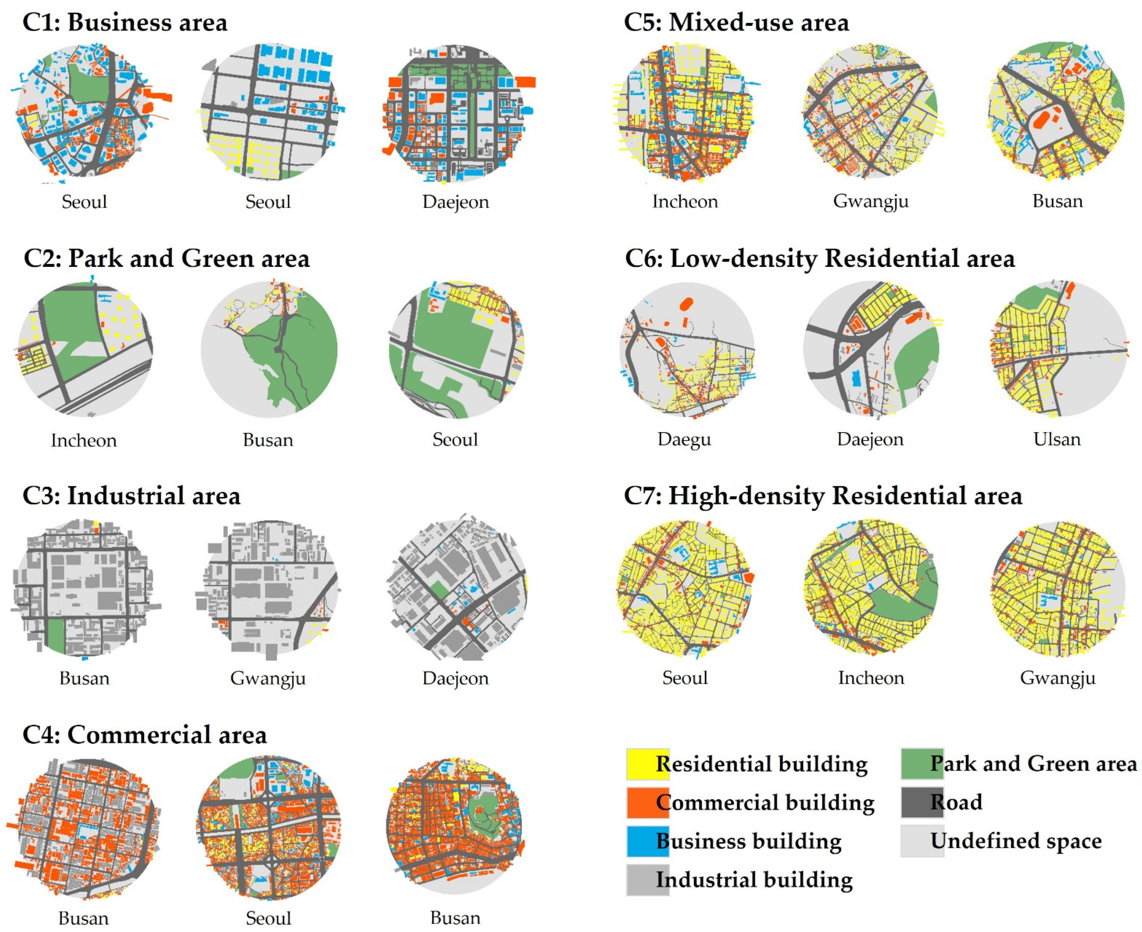
2.3. K-Means Clustering for Land-Use Clarification around AQMS

We applied K-means clustering to analyze the physical environment characteristics represented by individual PM measuring stations installed in urban areas. In other words, it analyzed the land-use characteristics of the surrounding environment where the measuring station is installed. The K-means clustering algorithm is a method that finds optimal clusters from data so that the averages of each cluster have independent relationships with each other, according to the number of clusters defined by the researcher in advance [56,57]. In this study, R version 4.1.0, and libraries such as kmeans, nortest, and dunn.test were used for clustering analysis.

Because the number of cluster is not analyzed in K-means clustering, the researcher must determine whether the analysis result is appropriate through post-hoc analysis. The normality test, Kruskal–Wallis Rank-Sum test, and Bonferroni post-hoc test were sequentially applied to ensure an objective basis for judgment rather than the subjectivity of the researcher. For the normality test, the Anderson–Darling test and the Shapiro–Francia test were used [58,59,60], and the rejection of the null hypothesis was judged conservatively. When the normality assumption was not satisfied through the normality test, the Kruskal–Wallis rank-sum test was performed among the nonparametric tests to analyze the characteristics of each cluster [61]. Finally, we applied the Bonferroni post-hoc test, which is used as a conservative post-hoc analysis method, to analyze the differences by cluster.

To categorize the surrounding environment of a PM measuring station in the urban area, the spatial range was limited to a radius of 500 m from the measuring station, and spatial data were constructed for this range. The reason for limiting it to 500 m is that the size of the neighborhood suggested by urban design theories, such as Clarence Perry and New Urbanism, is about 500 m in radius. The space-related variables were buildings and land-use, green and parks, roads, and the entropy index [62,63,64,65,66,67]. The reason for configuring these variables is that they can be used as a framework for analyzing urban form and land-use characteristics. The main variables were land use, mixed use, and street networks. Since PM is closely related to human activities, these variables are suitable for categorizing the environment surrounding the measuring station. For this reason, density, single or mixed land use, and road variables were set for clustering to find land-use patterns in the surrounding environment of a measuring station (

Table 1. Variables and Data Sources for Clustering.

Variables		Source
Density	Population	KOSIS(2017)
	Building Floor area	Road Name Address development system(2018) from Ministry of the Interior and Safety
Single Land use	Residential building area
	Business building area
	Commercial building area
	Industrial building area
	Parks and green area
Mixed land use	Entropy index
Road	Road area

).

2.4. Model Specification

We used two log-lin regression models to empirically verify the effects of each land-use type on fine dust. The first model examined the relationship between the daily PM10 average concentration and land-use type, while the second model explored the relationship between daily PM10 variability and land-use type.

Log-lin regression was applied for two reasons [68,69]. First, it is necessary to change the PM10 concentration distribution to a normal distribution through log transformation (Figure 3) because the average and variability of the daily PM10 concentrations are extremely right-skewed. Second, it is possible to interpret the coefficients of variables as rate of change for dependent variable by applying the log-lin model, which enables intuitive interpretation of the effects of independent variables on dependent variables. The coefficient of the model indicates the percentage change in the dependent variable when the individual independent variable changes by one unit [68,69].

The dependent variables in the two models were the daily mean concentrations and variability of PM10. The explanatory variables were composed of land use, seasonal, and macro or microclimate features. Furthermore, a region dummy was added as a control variable to reflect the characteristics of each city that are difficult to explain with the independent variables (

Table 2. Variables of the log-lin models.

Variables			Measurement	Unit	Source
Dependent Variables		Daily PM10 concentration	Average concentration of PM10 measured every hour	µg/m3	Korean AQMS data from AirKorea
		Daily PM10 variation	Variation of PM10 concentration measured every hour	-
Independent Variables	Land-use features	Business area	Predicted Type by K-means Clustering Analysis	dummy	National Spatial Information Portal from Ministry of Land, Infrastructure and Transport/Road Name Address development system from Ministry of the Interior and Safety
		Industrial area
		Commercial area
		Mixed area
		Residential with Low density
		Residential with High density
		Green area (reference)
	Seasonal features	Spring	March, April, May	dummy	Korean AQMS data from AirKorea
		Summer	June, July, August
		fall	September, October, November
		Winter (reference)	December, January, February
	Macro or Microclimate features	Temperature	Average of hourly recorded values per day	°C	Korean AWS data from KMA
		Precipitation		mm
		Windspeed		m/s
		PM2.5 from overseas		µg/m3	Korean AQMS data from AirKorea
Control Variables	Regional features	Seoul (reference)		dummy	Road Name Address development system from Ministry of the Interior and Safety
		Incheon
		Daejeon
		Daegu
		Gwangju
		Ulsan
		Busan

).

3. Results and Discussion

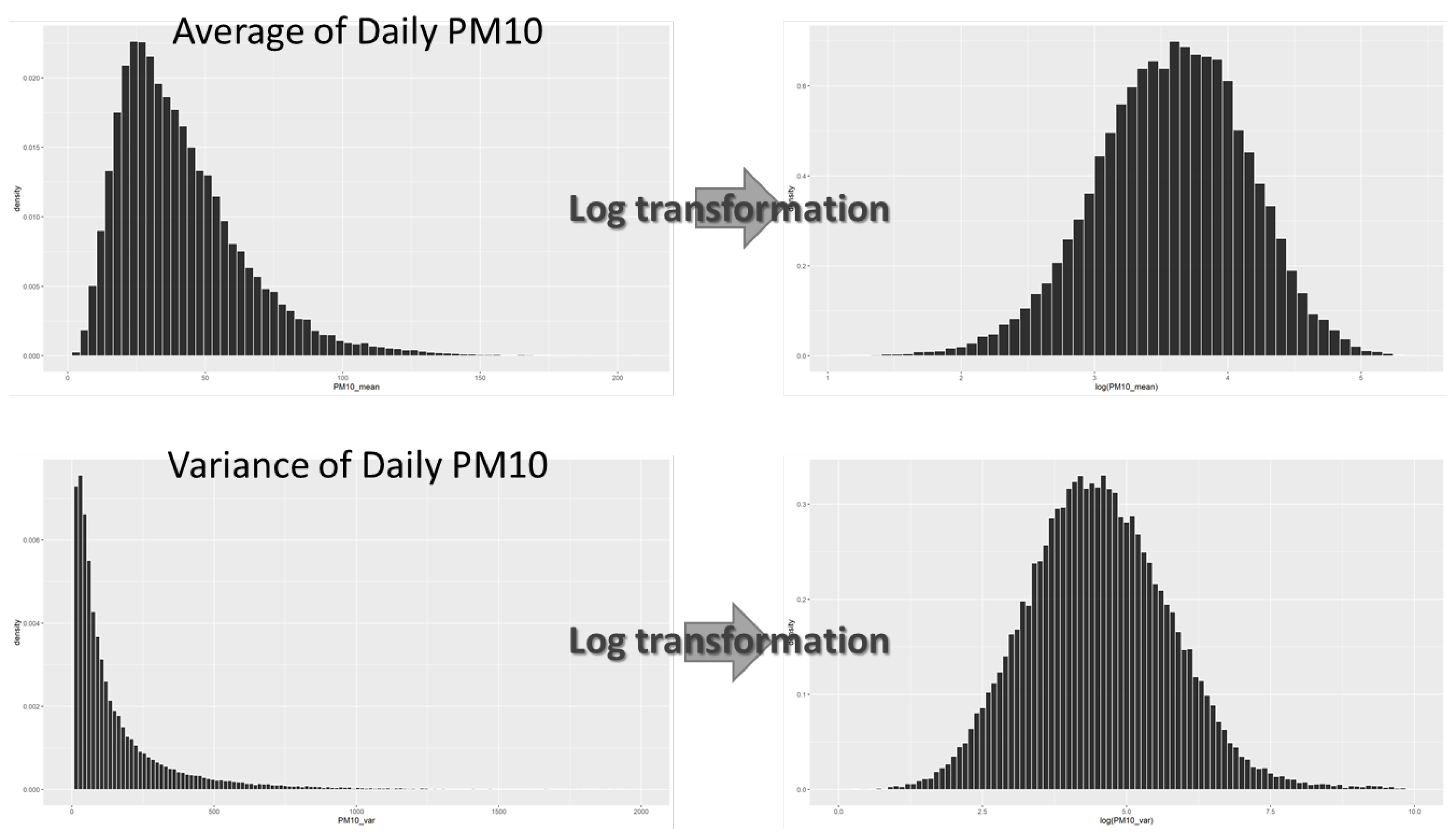
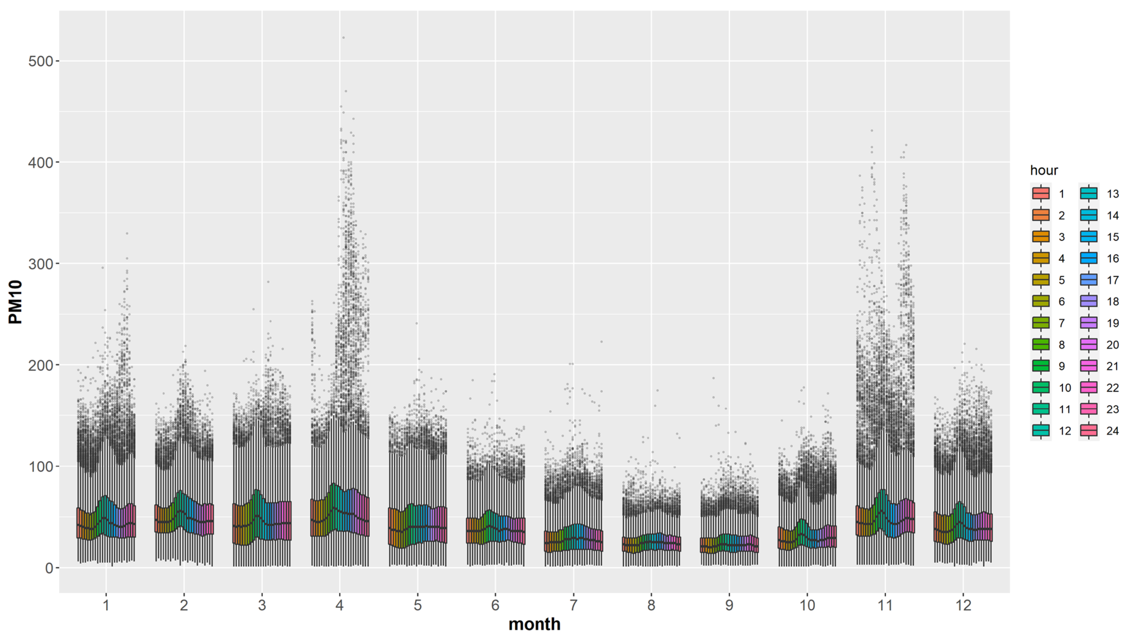
3.1. General Characteristics of PM10 Distribution

A boxplot of the hourly PM₁₀ concentration (µg/m³) distribution in metropolitan areas in South Korea in 2018 shows various patterns depending on the season and time (see Figure 4). The annual average concentration of PM10 measured in South Korea was 41.56 µg/m³, while the minimum value was 1 µg/m³ and the maximum value was 523 µg/m³, with a standard deviation of 774.53 µg/m³.

Note that the pattern of the PM₁₀ distribution varies according to the season. In South Korea, not only was the average concentration of PM₁₀ low in July, August, and September but its variability was also minimal. However, in February, April, November, and January, the average concentration of the PM was high (Appendix A), and in April, February, March, and November, the variability was relatively large (Appendix B). This is due to the climatic characteristics of the East Asian region. In general, summer is a season with little macroscopic atmospheric change, as the North Pacific high pressure with hot air is stably located near the Korean Peninsula, whereas, in autumn, the inflow of PM increases as the atmosphere flows from the west under the influence of westerly winds. Additionally, in April, yellow dust from Inner Mongolia flows into East Asia. In the spring season, it can be understood that the concentration of PM caused by yellow dust is high and the variability is significant.

Another characteristic of the PM10 distribution in South Korea is that it shows a certain pattern depending on the time. In the afternoon, when humans are active and the temperature rises, the PM concentration is high and the variability is large. Conversely, during late-night hours, when human activity and the temperature decrease, the PM concentration decreases as well. These patterns were found to be independent of the seasonal influences, indicating that PM in large cities is closely related to human activities.

3.2. Differences in the PM10 Level According to Land-Use Clarification

The K-means clustering algorithm was applied to analyze the land-use characteristics of 138 measuring stations installed in large cities in South Korea. Through repeated experiments through a Scree plot, it was determined that the seven clusters were appropriate (see Figure 5).

By applying the normality test, the land-use variables did not satisfy the null hypothesis of normality. Therefore, the nonparametric Kruskal–Wallis rank-sum test and post-hoc analysis were performed to verify the differences between clusters (see

Table 3. Analysis of normality and differences in cluster analysis.

	Overall	C1	C2	C3	C4	C5	C6	C7	Normality and Kruskal–Wallis Test
Population	17.706	8.611	11.991	1.588	10.343	23.710	12.814	27.315	(A.D.) A = 0.70768, p-value = 0.06333/ (S.F.) W = 0.97615, p-value = 0.01769/ (K.W.) chi-squared = 83.727, p-value ≤ 0.0001
Building Floor Area	0.2204	0.2045	0.1049	0.2368	0.3244	0.2562	0.1140	0.2617	(A.D.) A = 1.7413, p-value ≤ 0.001/ (K.W.) chi-squared = 85.631, p-value ≤ 0.0001
Residential Area	0.0983	0.0391	0.0515	0.0086	0.0456	0.1258	0.0606	0.1836	(A.D.) A = 0.94099, p-value = 0.01671/ (K.W.) chi-squared = 42.732, p-value ≤ 0.0001
Business Area	0.0248	0.0828	0.0204	0.0066	0.0386	0.0311	0.0144	0.0160	(A.D.) A = 3.8835, p-value ≤ 0.0001/ (K.W.) chi-squared = 66.993, p-value ≤ 0.0001
Commercial Area	0.0596	0.0548	0.0255	0.0075	0.1829	0.0785	0.0265	0.0452	(A.D.) A = 4.8815, p-value ≤ 0.0001/ (K.W.) chi-squared = 95.102, p-value ≤ 0.0001
Industrial Area	0.0377	0.0277	0.0076	0.2140	0.0573	0.0209	0.0126	0.0168	(A.D.) A = 26.082, p-value ≤ 0.0001/ (K.W.) chi-squared = 58.329, p-value ≤ 0.0001
Park and Green Area	0.0476	0.0359	0.2448	0.0193	0.0301	0.0127	0.0414	0.0443	(A.D.) A = 15.919, p-value ≤ 0.0001/ (K.W.) chi-squared = 42.732, p-value ≤ 0.0001
Entropy Index	0.3926	0.4587	0.4478	0.0606	0.4197	0.4621	0.4377	0.3383	(A.D.) A = 8.5061, p-value ≤ 0.0001/ (K.W.) chi-squared = 76.419, p-value ≤ 0.0001
Road Area	0.1670	0.2061	0.1212	0.0942	0.2212	0.1986	0.1301	0.1705	(A.D.) A = 0.5647, p-value = 0.1412/ (S.F.) W = 0.9842, p-value = 0.1027/ (K.W.) chi-squared = 74.632, p-value ≤ 0.0001

(1) Units: Squared kilometer for the area variables, and one thousand people for population. (2) A.D.: the Anderson–Darling test for normality; S.F.: the Shapiro–Francia test for normality; K.W.: Kruskal–Wallis Test as one of the nonparametric statistical methods. (3) The entropy index has a value between 0 and 1, with values closer to 0 indicating single land use, and those closer to 1 indicating mixed land use.

and the Appendix C). Consequently, the surrounding environment of the PM10 measurement stations was divided into seven types through cluster analysis and post-analysis (see Figure 6): business area (C1), park and green area (C2), industrial area (C3), commercial area (C4), mixed area (C5), low-density residential area (C6), and high-density residential area (C7). By land-use type, the mixed area (C5) had the most stations at 43, followed by the high-density residential area (C7) with 28 and the low-density residential area (C6) with 25, resulting in a total of 53 residential areas. Additionally, 12 parks and green areas (C2), industrial areas (C3), and commercial areas (C4) were drawn evenly, with six business areas (C1) found.

The difference in the daily mean concentration and variability of PM10 by cluster type was further tested using nonparametric ANOVA. After dividing the environment surrounding the measuring station into seven types, the average PM10 concentration was found to be high in industrial, commercial, and business areas, with the difference between the three groups being not statistically significant. The mixed- and high-density residential areas appeared next, with the parks and green areas and low-density residential areas showing the lowest average PM10 concentration (

Table 4. Differences in PM10 concentration and variability by cluster.

Cluster Type		Average of Daily PM10	Variance of Daily PM10	n
C1	Business Areas	43.6	253.1	2190
C2	Parks and Green Areas	38.9	206.7	4324
C3	Industrial Areas	44.4	280.4	3834
C4	Commercial Areas	43.6	258.0	4380
C5	Mixed areas	41.5	240.7	15,029
C6	Residential Areas with Low density	38.8	206.4	8057
C7	Residential Areas with High density	41.9	244.2	10,220

(1) For Average of Daily PM10. Bartlett Test for Average of Daily PM10: K-squared = 217.85, df = 6, p-value < 0.001. Kruskal–Wallis Rank-Sum Test for Average of Daily PM10: Chi-squared = 249.99, p-value < 0.001. (2) For Variance of Daily PM10. Bartlett Test for Variance of Daily PM10: K-squared = 732, df = 6, p-value < 0.001. Kruskal–Wallis Rank-Sum Test for Variance of Daily PM10: Chi-squared = 276.91, p-value < 0.001.

and Appendix D). The PM10 variability was similar to the mean concentration results but with one difference. The variability of industrial, commercial, and business areas was similar, while mixed areas showed higher variability than high-density residential areas. The parks and green areas and the low-density residential areas showed the lowest variability at a similar level (Table 4 and Appendix E).

These results are closely related to the generation of PM10 caused by urban activities. It was found that the concentration and variability of PM10 were large in land-use types with dense transportation (25%) and industrial (18%) activities [3]. Industrial activities and scattering dust due to wide roads are generated in industrial areas [36]. Therefore, it is understandable that the concentration and variability of PM10 in industrial areas are high. However, it is noteworthy that commercial and business areas do not differ from industrial areas in terms of PM10 levels. This means that in metropolitan cities, the activity itself is more important for PM10 generation than the type of urban activity, except for residential areas. In the residential area, the results were interesting. There is no difference in the concentration of PM10 by the density of residential areas, but the density is expected to affect the variability of PM10.

Meanwhile, what is interesting is the relationship between the mixed areas and PM10. In mixed areas, both the concentration and variability of PM10 were found to be lower than those of industrial, commercial, and business areas created as a single purpose land use. This suggests the possibility of reducing the impact of urban activities on the generation of PM through mixed land use.

3.3. The Relationship between PM10 and Land-Use Type Using Log-Linear Regression Models

3.3.1. The Correlation between Average Daily PM10 Concentration and Land-Use Type

The log-linear regression analysis was performed with the average daily PM10 concentration as the dependent variable, and the land-use type obtained from previous clustering analysis, seasonal dummy, microclimate features, and regional dummy as explanatory variables.

Table 5. Descriptive statistics.

Variables		min	mean	max	sd	n
Dependent variables	Average of Daily PM10	3.042	41.449	41.449	23.370	46,370
	Variation of Daily PM10	0.042	237.9	25,549	799.0	46,366
Land-use features	Business area	0.000	0.046	1.000	0.209	2190
	Industrial area	0.000	0.080	1.000	0.271	3834
	Commercial area	0.000	0.091	1.000	0.288	4380
	Mixed area	0.000	0.313	1.000	0.464	15,029
	Residential with Low density	0.000	0.168	1.000	0.374	8057
	Residential with High density	0.000	0.213	1.000	0.409	10,220
	Green area (reference)	0.000	0.090	1.000	0.286	4324
Seasonal features	Spring	0.000	0.249	1.000	0.432	11,948
	Summer	0.000	0.252	1.000	0.434	12,099
	Fall	0.000	0.254	1.000	0.435	12,188
	Winter	0.000	0.246	1.000	0.430	11,799
Macro or Microclimate features	Temperature	−16.60	13.53	34.40	10.50	47,650
	Precipitation	0.000	3.679	249.5	13.075	47,908
	Wind speed	0.000	1.874	14.900	1.112	47,627
	PM2.5 from overseas	3.292	17.293	108.3	11.844	48,034
Regional features	Seoul (reference)	0.000	0.298	1.000	0.457	14,296
	Incheon	0.000	0.151	1.000	0.358	7244
	Daejeon	0.000	0.078	1.000	0.268	3736
	Daegu	0.000	0.112	1.000	0.315	5357
	Gwangju	0.000	0.068	1.000	0.252	3285
	Ulsan	0.000	0.127	1.000	0.333	6098
	Busan	0.000	0.167	1.000	0.373	8018
Full sample		48,034

reports the descriptive statistics of the variables used in the analysis. We identified various factors that influenced the average concentration of PM10 (

Table 6. Log-Lin Regression Model on Average Daily PM10 Concentration.

Variables	Estimate	Std. Error	t-Value	Pr (>|t|)
Cluster Type (reference: Parks and Green areas)
Business areas	0.138	0.012	11.522	<0.001 ***
Industrial areas	0.133	0.010	12.748	<0.001 ***
Commercial areas	0.115	0.010	11.398	<0.001 ***
Mixed areas	0.045	0.008	5.685	<0.001 ***
Low-density residential areas	0.000	0.009	0.038	0.97
High-density residential areas	0.057	0.008	6.742	<0.001 ***
Season dummy (reference: winter)
Spring	0.087	0.008	10.594	<0.001 ***
Summer	−0.171	0.012	−14.101	<0.001 ***
Fall	−0.141	0.009	−16.531	<0.001 ***
Microclimate features
Temperature	−0.005	0.000	−11.375	<0.001 ***
Rain (mm)	−0.010	0.000	−59.849	<0.001 ***
Wind	−0.138	0.002	−61.598	<0.001 ***
PM2.5 from overseas	0.018	0.000	95.848	<0.001 ***
Region dummy (reference: Seoul)
Incheon	−0.014	0.007	−2.015	0.043 **
Daejeon	0.008	0.009	0.871	0.383
Daegu	0.061	0.008	7.977	<0.001 ***
Gwangju	0.001	0.009	0.158	0.874
Ulsan	0.18	0.008	23.215	<0.001 ***
Busan	0.156	0.007	23.351	<0.001 ***
Intercept	3.556	0.010	343.178	<0.001 ***

(1) (1) Sample = 44,127 (2) Maximum of VIF = 6.593 (3) Residual Standard Error = 0.4349 (4) F-statistics = 1541, DF = 19 and 44,103, p-value < 0.001 (5) R-squared = 0.4349, Adjusted R-squared = 0.3987. ** means p-value < 0.05, *** means p-value < 0.001.

). The cluster type, season dummy, microclimate feature, and region dummy all had effects on PM10 concentration. Since the log-lin model was analyzed, the coefficient value of each explanatory variable can be directly interpreted as percentage change for a dependent variable. Additionally, each explanatory variable as categorical data should be interpreted as an effect compared to the reference group. When focusing on the effect of land-use type as the main target variable, the average PM10 concentration in business areas was approximately 13.8% higher than in parks and green areas as the reference group. PM10 in industrial, commercial, mixed, and high-density residential areas was approximately 13.3%, 11.5%, 4.5%, and 5.7% higher, respectively, than that of parks and green areas. Nevertheless, there was no statistically significant difference in PM10 distribution between parks and green areas and low-density residential areas. The average PM10 concentration was found to be high in land-use types, such as business, industrial, and commercial areas, where human activities are continuously occurring or have characteristics that induce PM10. However, the PM10 concentration in mixed areas was approximately 4.5% higher than that in parks and green areas. This is because the difference is relatively small compared to other land-use types, assuming that human activities occur evenly in mixed areas, with relatively few human activities occurring in parks and green areas.

The seasonal and microclimatic variables were also found to affect the PM10 distribution. Compared to winter as the reference group, the average daily PM10 concentrations were approximately 8.7% higher in spring, 17.1% lower in summer, and 14.1% lower in autumn. These results are consistent with the PM10 distribution in South Korea (see Figure 4). As for the microclimate effect, it was found that the higher the daily average temperature, the heavier the rain, the faster the wind blows, and the lower the average daily PM10 concentration. Owing to Korea’s climate characteristics, it is difficult to understand why PM10 decreases as the temperature rises, with all other variables being equal. However, it can be understood that temperature has an effect in two directions. When the temperature is high, the surface temperature is also high and the atmospheric convection is active, which, thus, reduces PM10. Conversely, nitrogen oxide in the atmosphere creates air pollutants such as PM10 at high temperatures [68]. Temperature also has the effect of reducing PM10 levels. However, with respect to the magnitude of the effect, when the average temperature rises by one Celsius degree, the PM10 concentration is reduced by approximately 0.05%, which is less effective than other variables.

Regional factors were also found to affect the daily PM10 concentration. Compared to Seoul as the reference group, Incheon showed approximately 1.4% lower PM10 concentration, whereas Daegu, Ulsan, and Busan had approximately 6.1%, 18.6%, and 15.6% higher average concentration, respectively. Incheon is located in the western part of the Korean Peninsula and is adjacent to the West Sea (Figure 1); thus, it can be interpreted that PM10 concentration is lower than in Seoul due to the location factor. Meanwhile, Busan and Ulsan are adjacently located in the southeast of the Korean Peninsula. These cities have grown into South Korea’s representative coastal industrial metropolises. Busan and Ulsan have approximately 210,000 and 170,000 manufacturing workers. That is, approximately 380,000 workers who are engaged in manufacturing in this region, making up 47.88% of the total number of manufacturing workers in Korea (Appendix F). Manufacturing workers also account for approximately 18% of total workers in Daegu, which can be interpreted as affecting PM generation due to industrial characteristics (Appendix F). Similarly, it can be interpreted that the level of PM in South Korea is higher than in Seoul owing to location factors.

3.3.2. Correlation between Variability of Daily PM10 Concentration and Land-Use Type

For the log-linear regression analysis, the variance of the PM10 concentration measured every hour was defined as the variability of PM10 and used as a dependent variable. The explanatory variables consisted of the land-use type obtained from previous clustering analysis, seasonal dummy, microclimate features, and regional dummy. The log-linear regression analysis indicated that various factors influenced the daily PM10 variability (

Table 7. Log-Lin Regression Model on Variability of Daily PM10 Concentration.

Variables	Estimate	Std. Error	t-Value	Pr (>|t|)
Cluster Type (reference: Parks and Green areas)
Business areas	0.236	0.029	8.014	<0.001 ***
Industrial areas	0.348	0.026	13.558	<0.001 ***
Commercial areas	0.241	0.025	9.74	<0.001 ***
Mixed areas	0.126	0.019	6.468	<0.001 ***
Low-density residential areas	0.016	0.022	0.718	0.473
High-density residential areas	0.062	0.021	2.952	0.003 **
Season dummy (reference: winter)
Spring	0.405	0.020	20.17	<0.001 ***
Summer	−0.272	0.030	−9.106	<0.001 ***
Fall	−0.162	0.021	−7.74	<0.001 ***
Microclimate features
Temperature	−0.009	0.001	−8.873	<0.001 ***
Rain (mm)	−0.003	0.000	−7.461	<0.001 ***
Wind	−0.178	0.005	−32.457	<0.001 ***
PM2.5 from overseas	0.035	0.000	75.589	<0.001 ***
Region dummy (reference: Seoul)
Incheon	−0.129	0.017	−7.446	<0.001 ***
Daejeon	−0.137	0.021	−6.42	<0.001 ***
Daegu	0.140	0.019	7.452	<0.001 ***
Gwangju	−0.140	0.022	−6.401	<0.001 ***
Ulsan	0.214	0.020	10.876	<0.001 ***
Busan	0.063	0.016	3.847	<0.001 ***
Intercept	4.243	0.025	166.509	<0.001 ***

(1) Sample = 40,308 (2) Maximum of VIF = 6.593 (3) Residual Standard Error = 1.7 (4) F-statistics = 736.7, DF = 19 and 44,103, p-value < 0.001 (5) R-squared = 0.2409, Adjusted R-squared = 0.2406. ** means p-value < 0.05, *** means p-value < 0.001.

). The cluster type, season dummy, microclimate feature, and region dummy all had effects on the variability of PM10 concentration Since the log-lin model was analyzed, the coefficient value of each explanatory variable can be directly interpreted as percentage change for a dependent variable. Additionally, each explanatory variable as categorical data should be interpreted as an effect compared to the reference group. When estimating the effect of land-use type as the target variable of this study, we found that the PM10 variance was about 23.6% higher in business areas than in parks and green areas as the reference group. Additionally, the PM10 variability values in industrial, commercial, mixed, low-density residential, and high-density residential areas were approximately 34.8%, 34.8%, 24.1%, 12.6%, and 6.2% higher than that in parks and green areas, respectively. However, there was no statistically significant difference in the PM10 variability between parks and green areas and low-density residential areas. The PM10 variability showed a pattern similar to the previous analysis results. The variability was high in land-use types, where humans were active, thus generating PM10 depending on the intensity of human activity. The main human activities in cities are transportation and industrial activities [1,3,36], and a large amount of PM is generated in areas where these activities happen. In addition, it can be interpreted that the greater the difference in activity intensity over time, the more land use is created for a single purpose, and then the greater the variability in the PM10 concentration due to activity. Conversely, mixed areas showed a lower level of variability compared to the single purposed land use area. These results mean that the variability of PM10 concentration can be controlled through land use planning. Mixed land use is a very effective spatial planning strategy for variability of PM10 rather than single land use. Additionally, looking at the results for residential areas, reducing the intensity of land use will help in reducing PM10 concentration variability.

The seasonal and microclimate variables were also found to affect the daily PM10 variability. Compared to winter as the reference group, the daily PM10 variability was approximately 40.5% higher in spring, 27.2% lower in summer, and 16.2% lower in autumn. These results are consistent with the PM10 time-series pattern (see Figure 2). As for the microclimate effect, we found that the higher the temperature, the higher the precipitation, the faster the wind blows, and the lower the daily PM10 variability. Moreover, we found that the higher the concentration of PM2.5 from overseas, the higher the variability of PM in South Korea. This can be interpreted as reducing the PM10 variability if the condition of allowing PM to flow without accumulating is satisfied.

Regional factors were also found to have an impact on PM10 variability. Compared to Seoul as the reference group, Incheon, Daejeon, Gwangju, Daegu, Ulsan, and Busan showed less PM10 variability by approximately −12.9%, −13.7%, −14.0%, 14.0%, 21.4%, and 6.3%, respectively. In addition, the variability of PM10 due to urban activities is greater in the southeastern region of the Korean Peninsula than in other regions. It can be interpreted that cities with a relatively high manufacturing ratio, such as Busan, Ulsan, and Daegu (Appendix F), show greater variability in PM10 concentration.

4. Conclusions

4.1. Need to Reduce Exposure to PM or Adaptive Land-Use Planning

Based on the results obtained, it is necessary to lower the intensity of human activities that generate PM, as we found a statistically significant difference in PM concentration and variability in the business, commercial, industrial, and high-density residential areas compared to areas, such as parks and green areas, with less activity. In other words, although the intensity and type of activity differ depending on the characteristics of land use, the concentration of human activities causes high PM concentrations, thus increasing the risk of exposure to PM. Therefore, it is expected that PM levels can be reduced if the intensity of land use is lowered.

When considering the effects of each land-use type on the concentration and variability of PM, the effectiveness of a mixed land-use planning strategy was confirmed. In modern urban planning such as New Urbanism, mixed land-use strategies are advocated to create sustainable, pedestrian-friendly, and lively neighborhoods [65,66,70,71]. In this regard, this study supports the idea that a mixed land-use strategy can reduce the risk of exposure to high PM concentrations by dispersing PM generation in urban areas. Therefore, to reduce the occurrence and variability of PM, it is necessary to formulate and implement a mixed land-use strategy as a key land-use plan direction.

Furthermore, it is necessary that the land-use strategy secures sufficient open space. In the empirical analysis, parks and green areas, which represented the reference group, showed statistically significant differences in PM concentration and variability of PM compared to other land-use types, except for low-density residential areas. Compared to parks and green areas, low-density residential areas have very little PM effect, produce less PM, and do not accumulate PM due to sufficient open space and green cover. Therefore, it is necessary to secure sufficient open space in consideration of these effects in other land-use types.

4.2. Need to Make PM Reduction Guideline Considering Microclimate Characteristics

The microclimatic factors also affect PM concentrations and variability. The empirical analysis confirmed that PM concentration and variability decreased as the temperature rose, the wind blew faster, and rain fell. Therefore, spatial planning that can properly utilize microclimate factors in urban areas is required. This can be interpreted as the fact that PM does not accumulate and is blown away under suitable microclimate conditions. As various systems and guidelines were created to improve the poor urban environment during the Industrial Revolution, it is necessary to consider microclimatic factors in spatial planning, such as creating wind paths to reduce PM and secure sufficient sunlight.

4.3. Necessity of a Plan to Reduce Exposure to PM in Consideration of Season and Time

It is necessary to understand the various phenomena that occur when domestic and foreign factors are combined with season and time, and to establish an adaptive plan for PM that considers all these factors. East Asia, including Korea, experience yellow dust from Inner Mongolia for a long time, in March and April. During this period, in South Korea, media delivers news related to yellow dust, to urge caution. A similar strategy needs to be adopted for PM. With the popularity of the Internet and smartphones, real-time information on fine dust can be obtained, making it is possible to understand the PM behavior according to the season and their variability patterns in the morning and afternoon hours of the day, thus minimizing exposure to PM.

This study has the following limitations. We verified the relationship between PM and land-use type using data from 2018 for large cities in South Korea. However, since various climate characteristics are experienced every year because of climate change, it is necessary to use multi-year data to control for these macroscopic changes. Additionally, in this study, since one day was used as the unit of analysis, the effect of various times was not reflected. In addition, since PM10 is closely related to the emission of air pollutants by facilities, it is necessary to establish a more comprehensive LUR model by acquiring air pollutant emission data for each facility. Therefore, future research should apply spatiotemporal analysis to obtain research results that reflect spatiotemporal characteristics along with a more rigorous analysis.

References

1. World Health Organization Regional Office for Europe. Review of Evidence on Health Aspects of Air Pollution—REVIHAAP Project: Technical Report; World Health Organization Regional Office for Europe: Copenhagen, Denmark, 2013. [Google Scholar]
2. World Health Organization Regional Office for Europe. Health Risks of Air Pollution in Europe—HRAPIE Project; World Health Organization Regional Office for Europe: Copenhagen, Denmark, 2013. [Google Scholar]
3. Karagulian, F.; Belis, C.A.; Dora, C.F.C.; Prüss-Ustün, A.M.; Bonjour, S.; Adair-Rohani, H.; Amann, M. Contributions to cities’ ambient particulate matter (PM): A systematic review of local source contributions at global level. Atmos. Environ. 2015, 120, 475–483. [Google Scholar] [CrossRef]
4. OECD. The Economic Consequences of Outdoor Air Pollution; OECD Publishing: Paris, France, 2016. [Google Scholar]
5. World Health Organization. Global Health Observatory. Available online: https://www.who.int/data/gho/data/themes/theme-details/GHO/air-pollution (accessed on 16 September 2021).
6. Chen, L.; Bai, Z.; Kong, S.; Han, B.; You, Y.; Ding, X.; Du, S.; Liu, A. A land use regression for predicting NO2 and PM10 concentrations in different seasons in Tianjin region, China. J. Environ. Sci. 2010, 22, 1364–1373. [Google Scholar] [CrossRef]
7. Pope, C.A.; Burnett, R.T.; Thun, M.J.; Calle, E.E.; Krewski, D.; Ito, K.; Thurston, G.D. Lung cancer, cardiopulmonary mortality, and long-term exposure to fine particulate air pollution. JAMA 2002, 287, 1132–1141. [Google Scholar] [CrossRef] [Green Version]
8. Eeftens, M.; Tsai, M.-Y.; Ampe, C.; Anwander, B.; Beelen, R.; Bellander, T.; Cesaroni, G.; Cirach, M.; Cyrys, J.; de Hoogh, K.; et al. Spatial Variation of PM2.5, PM10, PM2.5 Absorbance and PM Coarse Concentrations between and within 20 European Study Areas and the Relationship with NO2—Results of the ESCAPE Project. Atmos. Environ. 2012, 62, 303–317. [Google Scholar] [CrossRef] [Green Version]
9. Allan, J.D.; Williams, P.I.; Morgan, W.T.; Martin, C.L.; Flynn, M.J.; Lee, J.; Nemitz, E.; Phillips, G.J.; Gallagher, M.W.; Coe, H. Contributions from transport, solid fuel burning and cooking to primary organic aerosols in two UK cities. Atmos. Chem. Phys. 2010, 10, 647–668. [Google Scholar] [CrossRef] [Green Version]
10. Lanz, V.; Alfarra, M.; Baltensperger, U.; Buchmann, B.; Hueglin, C.; Prevot, A. Source apportionment of submicron organic aerosols at an urban site by factor analytical modeling of aerosol mass spectra. Atmos. Chem. Phys. 2007, 7, 1503–1522. [Google Scholar] [CrossRef] [Green Version]
11. Karner, A.A.; Eisinger, D.S.; Niemeier, D.A. Near-Roadway Air Quality: Synthesizing the Findings from Real-World Data. Environ. Sci. Technol. 2010, 44, 5334–5344. [Google Scholar] [CrossRef]
12. Massoli, P.; Fortner, E.C.; Canagaratna, M.R.; Williams, L.R.; Zhang, Q.; Sun, Y.; Schwab, J.J.; Trimborn, A.; Onasch, T.B.; Demerjian, K.L.; et al. Pollution Gradients and Chemical Characterization of Particulate Matter from Vehicular Traffic near Major Roadways: Results from the 2009 Queens College Air Quality Study in NYC. Aerosol Sci. Technol. 2012, 46, 1201–1218. [Google Scholar] [CrossRef]
13. Bayer-Oglesby, L.; Schindler, C.; Arx, M.; Braun-Fahrländer, C.; Keidel, D.; Rapp, R.; Künzli, N.; Braendli, O.; Burdet, L.; Liu, L.-J.; et al. Living near Main Streets and Respiratory Symptoms in Adults the Swiss Cohort Study on Air Pollution and Lung Diseases in Adults. Am. J. Epidemiol. 2007, 164, 1190–1198. [Google Scholar] [CrossRef] [Green Version]
14. Beelen, R.; Raaschou-Nielsen, O.; Stafoggia, M.; Andersen, Z.J.; Weinmayr, G.; Hoffmann, B.; Wolf, K.; Samoli, E.; Fischer, P.; Nieuwenhuijsen, M.; et al. Effects of long-term exposure to air pollution on natural-cause mortality: An analysis of 22 European cohorts within the multicentre ESCAPE project. Lancet 2014, 383, 785–795. [Google Scholar] [CrossRef]
15. Alam, M.S.; McNabola, A. Exploring the modeling of spatiotemporal variations in ambient air pollution within the land use regression framework: Estimation of PM10 concentrations on a daily basis. J. Air Waste Manag. Assoc. 2015, 65, 628–640. [Google Scholar] [CrossRef] [PubMed]
16. Brauer, M.; Lencar, C.; Tamburic, L.; Koehoorn, M.; Demers, P.; Karr, C. A cohort study of traffic-related air pollution impacts on birth outcomes. Environ. Health Perspect. 2008, 116, 680–686. [Google Scholar] [CrossRef] [PubMed] [Green Version]
17. Janssen, S.; Dumont, G.; Fierens, F.; Mensink, C. Spatial interpolation of air pollution measurements using CORINE land cover data. Atmos. Environ. 2008, 42, 4884–4903. [Google Scholar] [CrossRef]
18. Jerrett, M.; Arain, A.; Kanaroglou, P.; Beckerman, B.; Potoglou, D.; Sahsuvaroglu, T.; Morrison, J.; Giovis, C. A review and evaluation of intraurban air pollution exposure models. J. Expo. Sci. Environ. Epidemiol. 2005, 15, 185–204. [Google Scholar] [CrossRef]
19. Kim, E.; Park, H.; Park, E.A.; Hong, Y.-C.; Ha, M.; Kim, H.-C.; Ha, E.-H. Particulate matter and early childhood body weight. Environ. Int. 2016, 94, 591–599. [Google Scholar] [CrossRef]
20. Künzli, N.; Jerrett, M.; Mack, W.J.; Beckerman, B.; LaBree, L.; Gilliland, F.; Thomas, D.; Peters, J.; Hodis, H.N. Ambient air pollution and atherosclerosis in Los Angeles. Environ. Health Perspect. 2005, 113, 201–206. [Google Scholar] [CrossRef]
21. Liu, W.; Li, X.; Chen, Z.; Zeng, G.; León, T.; Liang, J.; Huang, G.; Gao, Z.; Jiao, S.; He, X.; et al. Land use regression models coupled with meteorology to model spatial and temporal variability of NO2 and PM10 in Changsha, China. Atmos. Environ. 2015, 116, 272–280. [Google Scholar] [CrossRef]
22. Miri, M.; Ghassoun, Y.; Dovlatabadi, A.; Ebrahimnejad, A.; Löwner, M.-O. Estimate annual and seasonal PM1, PM2.5 and PM10 concentrations using land use regression model. Ecotoxicol. Environ. Saf. 2019, 174, 137–145. [Google Scholar] [CrossRef]
23. Wrenn, D.H.; Sam, A.G. Geographically and temporally weighted likelihood regression: Exploring the spatiotemporal determinants of land use change. Reg. Sci. Urban Econ. 2014, 44, 60–74. [Google Scholar] [CrossRef]
24. Ng, E. Policies and technical guidelines for urban planning of high-density cities—Air ventilation assessment (AVA) of Hong Kong. Build. Environ. 2009, 44, 1478–1488. [Google Scholar] [CrossRef]
25. Briggs, D.; Collins, S.; Elliott, P.; Fischer, P.; Kingham, S.; Lebret, E.; Pryl, K.; Reeuwijk, H.; Smallbone, K.; Veen, A. Mapping Urban Air Pollution Using GIS: A Regression-Based Approach. Int. J. Geogr. Inf. Sci. 1997, 11, 699–718. [Google Scholar] [CrossRef] [Green Version]
26. Dons, E.; Van Poppel, M.; Kochan, B.; Wets, G.; Int Panis, L. Modeling temporal and spatial variability of traffic-related air pollution: Hourly land use regression models for black carbon. Atmos. Environ. 2013, 74, 237–246. [Google Scholar] [CrossRef]
27. Hoek, G.; Beelen, R.; de Hoogh, K.; Vienneau, D.; Gulliver, J.; Fischer, P.; Briggs, D. A review of land-use regression models to assess spatial variation of outdoor air pollution. Atmos. Environ. 2008, 42, 7561–7578. [Google Scholar] [CrossRef]
28. Briggs, D.J.; de Hoogh, C.; Gulliver, J.; Wills, J.; Elliott, P.; Kingham, S.; Smallbone, K. A regression-based method for mapping traffic-related air pollution: Application and testing in four contrasting urban environments. Sci. Total Environ. 2000, 253, 151–167. [Google Scholar] [CrossRef]
29. Gulliver, J.; Briggs, D.J. Time-space modeling of journey-time exposure to traffic-related air pollution using GIS. Environ. Res. 2005, 97, 10–25. [Google Scholar] [CrossRef]
30. Gilbert, N.L.; Goldberg, M.S.; Beckerman, B.; Brook, J.R.; Jerrett, M. Assessing spatial variability of ambient nitrogen dioxide in Montréal, Canada, with a land-use regression model. J. Air Waste Manag. Assoc. 2005, 55, 1059–1063. [Google Scholar] [CrossRef] [PubMed] [Green Version]
31. Hystad, P.; Setton, E.; Cervantes-Larios, A.; Poplawski, K.; Deschenes, S.; Martin, R.; Van Donkelaar, A.; Atari, O.; Demers, P.A. Canada Wide Land-use Regression Models Created from Fixed Site Monitors and Validated with Independent City-specific Measurements. Epidemiology 2011, 22, S214. [Google Scholar] [CrossRef]
32. Novotny, E.V.; Bechle, M.J.; Millet, D.B.; Marshall, J.D. National satellite-based land-use regression: NO2 in the United States. Environ. Sci. Technol. 2011, 45, 4407–4414. [Google Scholar] [CrossRef]
33. Ross, Z.; English, P.B.; Scalf, R.; Gunier, R.; Smorodinsky, S.; Wall, S.; Jerrett, M. Nitrogen dioxide prediction in Southern California using land use regression modeling: Potential for environmental health analyses. J. Expo. Sci. Environ. Epidemiol. 2006, 16, 106–114. [Google Scholar] [CrossRef]
34. Amini, H.; Taghavi-Shahri, S.M.; Henderson, S.B.; Naddafi, K.; Nabizadeh, R.; Yunesian, M. Land use regression models to estimate the annual and seasonal spatial variability of sulfur dioxide and particulate matter in Tehran, Iran. Sci. Total. Environ. 2014, 488, 343–353. [Google Scholar] [CrossRef]
35. Kashima, S.; Yorifuji, T.; Tsuda, T.; Doi, H. Application of land use regression to regulatory air quality data in Japan. Sci. Total. Environ. 2009, 407, 3055–3062. [Google Scholar] [CrossRef] [PubMed]
36. Kim, H. Land Use Impacts on Particulate Matter Levels in Seoul, South Korea: Comparing High and Low Seasons. Land 2020, 9, 142. [Google Scholar] [CrossRef]
37. Shi, Y.; Lau, K.K.-L.; Ng, E. Developing Street-Level PM2.5 and PM10 Land Use Regression Models in High-Density Hong Kong with Urban Morphological Factors. Environ. Sci. Technol. 2016, 50, 8178–8187. [Google Scholar] [CrossRef] [PubMed]
38. Stedman, J.R.; Vincent, K.J.; Campbell, G.W.; Goodwin, J.W.L.; Downing, C.E.H. New high resolution maps of estimated background ambient NOx and NO2 concentrations in the U.K. Atmos. Environ. 1997, 31, 3591–3602. [Google Scholar] [CrossRef]
39. Arain, M.A.; Blair, R.; Finkelstein, N.; Brook, J.R.; Sahsuvaroglu, T.; Beckerman, B.; Zhang, L.; Jerrett, M. The use of wind fields in a land use regression model to predict air pollution concentrations for health exposure studies. Atmos. Environ. 2007, 41, 3453–3464. [Google Scholar] [CrossRef]
40. Blanchard, C.L.; Tanenbaum, S.; Hidy, G.M. Spatial and temporal variability of air pollution in Birmingham, Alabama. Atmos. Environ. 2014, 89, 382–391. [Google Scholar] [CrossRef]
41. AirKorea. Available online: https://www.airkorea.or.kr (accessed on 16 September 2021).
42. “Asian Dust” Wikipedia. Available online: https://en.wikipedia.org/wiki/Asian_Dust (accessed on 16 September 2021).
43. “Siberian High” Wikipedia. Available online: https://en.wikipedia.org/wiki/Siberian_High (accessed on 16 September 2021).
44. “North Pacific High” Wikipedia. Available online: https://en.wikipedia.org/wiki/North_Pacific_High (accessed on 16 September 2021).
45. Lee, S.; Ho, C.-H.; Lee, Y.G.; Choi, H.-J.; Song, C.-K. Influence of transboundary air pollutants from China on the high-PM10 episode in Seoul, Korea for the period 16–20 October 2008. Atmos. Environ. 2013, 77, 430–439. [Google Scholar] [CrossRef]
46. Joint Research Project for Long–Range Transboundary Air Pollutants in Northeast Asia. In Summary Report of the 4th Stage (2013–2017) LTP Project; Research Report to National Institute of Environmental Research: Incheon, Korea, 2019.
47. Park, S.; Kim, M.; Im, J. Estimation of Ground-level PM10 and PM2.5 Concentrations Using Boosting-based Machine Learning from Satellite and Numerical Weather Prediction Data. Korean J. Remote Sens. 2021, 37, 321–335. [Google Scholar]
48. Ryu, H.-W.; Jang, D.-H. A Study on the Conformity Assessment of GWR Model through Analyzing the Correlation between Fine Particles(PM10) Concentration and Land-cover. J. Assoc. Korean Photo Geogr. 2019, 29, 73–84. [Google Scholar] [CrossRef]
49. Krynicka, J.; Drzeniecka-Osiadacz, A. Analysis of Variability in PM 10 Concentration in the Wrocław Agglomeration. Pol. J. Environ. Stud. 2013, 22, 1091–1099. [Google Scholar]
50. Honderich, T. The Oxford Companion to Philosophy; Oxford University Press: Oxford, UK, 2005; p. 703. [Google Scholar]
51. Babbie, E. The Practice of Social Research, 12th ed.; Cengage Learning: Boston, MA, USA, 2009; p. 625. [Google Scholar]
52. Gu, P.; Li, H.Z.; Ye, Q.; Robinson, E.S.; Apte, J.S.; Robinson, A.L.; Presto, A.A. Intracity Variability of Particulate Matter Exposure Is Driven by Carbonaceous Sources and Correlated with Land-Use Variables. Environ. Sci. Technol. 2018, 52, 11545–11554. [Google Scholar] [CrossRef] [PubMed]
53. KOSIS. Available online: https://kostat.go.kr/ (accessed on 16 September 2021).
54. KMA. Available online: https://www.weather.go.kr/ (accessed on 16 September 2021).
55. R Core Team: A Language and Environment for Statistical Computing; R Foundation for Statistical Computing: Vienna, Austria, 2020.
56. Kodinariya, T.M.; Makwana, P.R. Review on determining number of Cluster in K-Means Clustering. Int. J. Mol. Sci. 2013, 1, 90–95. [Google Scholar]
57. MacQueen, J. Some methods for classification and analysis of multivariate observations. In Proceedings of the Fifth Berkeley Symposium on Mathematical Statistics and Probability; University of California Press: Berkeley/Los Angeles, CA, USA, 1967; Volume 1, pp. 281–297. [Google Scholar]
58. D’Agostino, R.B. Goodness-of-Fit-Techniques; CRC Press: New York, NY, USA, 1986; Volume 68. [Google Scholar]
59. Thode, H.C. Testing for Normality; CRC Press: Boca Raton, FL, USA, 2002. [Google Scholar]
60. Royston, P. A pocket-calculator algorithm for the shapiro-francia test for non-normality: An application to medicine. Stat. Med. 1993, 12, 181–184. [Google Scholar] [CrossRef] [PubMed]
61. Hollander, M.; Wolfe, D. Nonparametric Statistical Methods; John Wiley & Sons: New York, NY, USA, 1999. [Google Scholar]
62. Ewing, R.; Handy, S. Measuring the unmeasurable: Urban design qualities related to walkability. J. Urban Des. 2009, 14, 65–84. [Google Scholar] [CrossRef]
63. Ewing, R.H.; Clemente, O.; Neckerman, K.M.; Purciel-Hill, M.; Quinn, J.W.; Rundle, A. Measuring Urban Design: Metrics for Livable Places; Springer: Berlin/Heidelberg, Germany, 2013; Volume 200. [Google Scholar]
64. Hamidi, S.; Ewing, R.; Preuss, I.; Dodds, A. Measuring sprawl and its impacts: An update. J. Plan. Educ. Res. 2015, 35, 35–50. [Google Scholar] [CrossRef]
65. Kim, H.; Ahn, K.-H. The Effects of Compact City Planning Strategies on Commuting Distance of Differenct Income Levels: Focused on Seoul, Korea. J. Urban. Des. Insitute Korea 2011, 12, 55–70. [Google Scholar]
66. Kim, H.; Ahn, K.-H.; Kwon, Y.-S. The Effects of Residential Environmental Factors on Personal Walking Probability—Focused on Seoul. J. Urban. Des. Insitute Korea 2014, 15, 5–18. [Google Scholar]
67. Southworth, M. Walkable suburbs?: An evaluation of neotraditional communities at the urban edge. J. Am. Plan. Assoc. 1997, 63, 28–44. [Google Scholar] [CrossRef]
68. Gelman, A.; Hill, J.; Vehtari, A. Regression and Other Stories; Cambridge University Press: Cambridge, UK, 2020. [Google Scholar]
69. Gujarati, D.N.; Porter, D.C.; Gunasekar, S. Basic Econometrics; Tata McGraw-Hill Education: Boston/NewYork, NY, USA, 2012. [Google Scholar]
70. CNU. Charter of the new urbanism. Bull. Sci. Technol. Soc. 2000, 20, 339–341. [Google Scholar] [CrossRef] [Green Version]
71. McCormack, G.R.; Shiell, A. In search of causality: A systematic review of the relationship between the built environment and physical activity among adults. Int. J. Behav. Nutr. Phys. Act. 2011, 8, 1–11. [Google Scholar] [CrossRef] [Green Version]
Figure 1. Research subject: Seven megacities in South Korea.
Land 11 00023 g001
Figure 2. Observatory and Land-use Characteristics in seven metropolitan cities.
Land 11 00023 g002
Figure 3. Distribution of dependent variables and log transformation.
Land 11 00023 g003
Figure 4. Boxplot of Daily PM10 Concentration in 2018.
Land 11 00023 g004
Figure 5. Scree Plot: internal variance change by the number of clusters.
Land 11 00023 g005
Figure 6. Representative case areas for each cluster: Each circle represents an area corresponding to a radius of 500 m from the AQMS. The AQMSs are located at the center of the circles. Whether the cluster analysis was performed properly can be checked through the visualization of land use around the AQMS.
Land 11 00023 g006