Abstract
The impact of the pandemic caused by COVID-19 on urban pollution in our cities is a proven fact, although its mechanisms are not known in great detail. The change in urban mobility patterns due to the restrictions imposed on the population during lockdown is a phenomenon that can be parameterized and studied from the perspective of spatial analysis. This study proposes an analysis of the guiding parameters of these changes from the perspective of spatial analysis. To do so, the case study of the city of Cartagena, a medium-sized city in Spain, has been analyzed throughout the period of mobility restrictions due to COVID-19. By means of a geostatistical analysis, changes in urban mobility patterns and the modal distribution of transport have been correlated with the evolution of environmental air quality indicators in the city. The results show that despite the positive effect of the pandemic in its beginnings on the environmental impact of urban mobility, the changes generated in the behavior patterns of current mobility users favor the most polluting modes of travel in cities.
1. Introduction
Air pollution in cities and rural areas around the world causes seven million premature deaths each year, with more than 400,000 in Europe alone [1,2]. In this context, transport accounts for 25% of greenhouse gases of the planet, with 70% of these gases produced by urban mobility in the form of cars, buses, vans, etc. [3,4].
It is true that urban pollution is not only due to issues arising from mobility and transport [5], as it is also linked to other activities, such as industry or the evolution of climatological variables, as has been detected in some cities [6,7]. Some of its causes, such as in the case of suspended solids, are not even anthropogenic, but can even come from natural elements [8].
However, most experts agree that pollution from urban mobility is currently the greatest challenge in relation to the future of air quality in cities [9,10] and its analysis through the indicator PM 2.5 the most effective way for its investigation [11,12,13]. In this context, it is important to bear in mind that we are facing a phenomenon of growing importance for some time in large cities around the world [14], which in the case of Europe is now also beginning to spread to medium-sized cities [15,16,17]. This argument is clearly supported by the seasonality in the values of the air quality measurement stations in many cities, in which periodic hourly and weekly behavior is reproduced with patterns very similar to those of traffic congestion [18].
In the last two years, the pandemic caused by the SARS-CoV-2 virus has brought about a very profound change in our society’s way of life at all levels. One of the aspects on which the pandemic has had a greater impact has been the field of urban mobility, due to the restrictions imposed in many countries. This has caused a temporary transformation of mobility patterns in cities, the impact of which is only partially known. At a general level, the first studies on the matter highlighted that, during the time of the greatest restrictions on mobility in cities, pollution levels fell by 50% in developed countries [19,20].
Nevertheless, these first figures are only part of the phenomenon, since the subsequent changes caused by the pandemic in the behavior patterns of urban mobility are not limited to the transitory impact of the initial reduction of polluting gases caused by people remaining at home due to lockdown. The capacity restrictions in public transport, the greater use of private vehicles because of the psychological effect of the possibility of contagion, or the change in the lifestyle habits of users throughout this past and present period have had effects that should also be analyzed from a broader perspective at the environmental level.
However, this issue is far from simple to analyze as it implies knowledge of the details of COVID-19 pandemic impact in the areas related to the behavior patterns of urban mobility and application to the field of environmental impact. In such a context, numerous studies have already appeared using different methodological approaches. A traditional approach involves the use of surveys combined with the analysis of air quality indicators [21,22,23]. An interesting variant within that approach is the growing use of apps to know the trends of user mobility through the use of information technologies [24]. It is also common to find mathematical models that allow to correlate global indicators of transport use with statistically inferred environmental conditions [25,26,27]. A more sophisticated approach to predict future polluting scenarios that has been used recently is to incorporate the spatial dimension by analyzing heat islands in cities [28]. Within this field, the use of sustainability indices is a tool that is being increasingly used to correlate urban mobility and environmental impact in cities [29,30,31]. This type of spatial analysis by means of indicators is typically very useful, albeit with significant shortcomings when, for example, analyzing the changing modal distribution of urban mobility [32,33]. In this sense, several mathematical and statistical models can be incorporated to improve per region analysis and perform comparative studies [34].
However, the complexity of the pandemic requires approaching the analysis of its impacts from a perspective more adapted to the boundary conditions that have occurred than that offered by traditional analyses. In this sense, spatial analysis using geostatistical tools can be of great help to understand, in the first place, what change has occurred in the behavior patterns of urban mobility during the pandemic, and subsequently, to correlate that change with the effects that it has on mobility-related behavioral habits of individuals at an environmental level in cities.
To address this, we have studied the urban mobility patterns in the city of Cartagena (southeast Spain) during the pandemic from the perspective of spatial statistical analysis. Urban mobility patterns reflecting behavioral motifs in the city before and during the pandemic have been contrasted by means of GIS spatial analysis indicators. These patterns have also been statistically correlated at the spatial level in the city using geostatistical analysis tools to infer the region-specific evolution of the different environmental impacts caused by the pandemic.
2. Methodology
2.1. Area of Study and Data Source
The study area is located in Cartagena, a medium-sized city in the southeast of Spain. Assessment of this phenomenon in a city of this category is not a random decision. Cartagena is a city that, due to its size, allows access to a critical mass of data on key pertinent variables, thus enabling robust statistical analysis without having to address the difficulty of handling large numbers of variables and data that would surely be involved in the context of a similar analysis in major European or American capital cities [35].
The city has several public transport alternatives such as urban and intercity buses (90,000 trips per day), medium and long-distance trains, and a complete taxi service. The size of the city means that the private-hire driver companies (VTCs) sector has yet to acquire sufficient critical mass to be considered as a relevant transport alternative, which makes it possible to simplify the analysis, assuming that all mobility linked to that option is provided by the taxi service. In the same way, private transport coexists with some current transport alternatives based on the concept of a collaborative economy, such as car sharing or carpooling, with incipient commercial platforms which have a minor presence in the modal distribution of mobility in the city. This implies that private transport can be assumed to correspond to the traditional use of transport with a self-owned vehicle with almost 200,000 trips per day.
On the other hand, as Cartagena is a touristic and university city (the municipality has a registered population of about 220,000 inhabitants plus a floating population of another 100,000 inhabitants linked to tourism), it has an important endowment of bike lanes, and new transport alternatives are developing, such as personal mobility vehicles, without being a particularly noteworthy figure within the set of bike lane users (representing this set of alternatives almost 35,000 trips per day). Last, pedestrian movements constitute a major component of mobility, representing 360,000 of the 700,000 total trips that are made in the city on a daily basis. The analysis will focus on the urban perimeter shown in Figure 1.
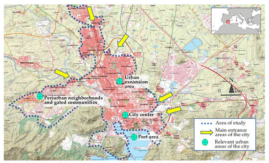
Figure 1.
Delineation of the area of study (urban area of the city of Cartagena).
Although tourism is a quite relevant activity in the city, regarding the seasonality of the data, it should be noted that the urban tourist offering in the city of Cartagena is quite seasonally adjusted. Therefore, there are no strong distortions regarding possible specific concentrations derived from the high tourism season. We must also note the existence of daily arrivals of cruise ships with several thousand tourists to the city’s seafront. However, the environmental impact of cruise ships that dock in the urban area of the port is quite reduced because of winds from the land-sea direction, which therefore prevents these emissions from entering the city.
The data used in relation to public transport and the use of private vehicles have been obtained from the information provided by the concessionaires regarding public transport by bus, the associations of taxi drivers, and the traffic analyses periodically carried out by the City Council in several of its streets through the municipal traffic control center. As for the information on pedestrian mobility, by bicycle and through personal mobility vehicles, the data have been obtained through a series of surveys carried out during the development of the Sustainable Urban Mobility Plan of the city of Cartagena through apps with georeferenced information systems (see Figure 2) that allowed to obtain spatial information on the itineraries used, the frequencies of use, and the profiles of non-users (see Figure 3).
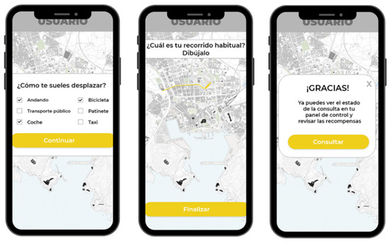
Figure 2.
Apps with georeferenced information used for the development of surveys in Cartagena.
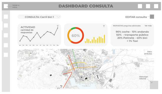
Figure 3.
Example of survey software for spatial analysis of bike lane activity during the pandemic.
2.2. GIS Indicators of Urban Mobility Spatial Patterns and Environmental Impact Assessment
For the purposes of this study, a spatial discretization of the urban area of the city has first been carried out. This process of compartmentalizing the urban continuum has been carried out based on the administrative structure of the city’s neighborhoods (mainly taking into account the urban and social configuration of the urban fabric). Specific sectors derived from urban configurations that require a singular treatment due to having specific characteristics (university areas, industrial estates, hospital spaces or large facilities, etc.) were subsequently added. The results obtained can be seen in Figure 4.
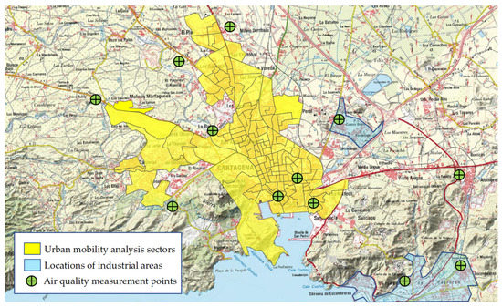
Figure 4.
Compartmentalization of the city of Cartagena into sectors according to the criteria described in the text.
Cartagena is also a city with an important industrial activity. In this sense, industrial zones have been identified on the maps in the revised version of the article. These areas were not considered within the scope of analysis to avoid a possible bias in the results, as they are also located outside the urban environment analyzed, so their associated traffic cannot be considered exactly urban mobility, but rather inter-urban or periurban movements. What will be studied in more detail is the contrast between the pedestrianized historic center of the city and the expansion areas of the city with heavy traffic loads.
Analysis has been limited to urbanized areas and with some interest for the study of phenomena related to urban mobility (therefore discarding the peri-urban areas of interest for the purposes of inter-urban mobility). The heterogeneous size of the sectors corresponds to different levels of population density and urban structure in relation to mobility. Small sectors tend to be located in areas with a high concentration of population or traffic in the city center. Larger sectors are generally located in areas of lower density, but with some road traffic to the city or with transitional pedestrian mobility between different sectors. In these urban sectors, indicators related to the different modal alternatives for urban mobility, as well as an indicator related to the environmental situation in the city, have been computed and spatially analyzed. The indicators used are described below.
2.2.1. Private Vehicle Use Density Index (PVUD)
This indicator assesses the evolution of the density of private vehicle use in a sector. Through the measurements and gauges of the City Council’s traffic control center in the different streets of the city, the level of traffic density in each of the sectors has been evaluated, comparing the existing values for the years 2019, 2020, and 2021. The indicator is formulated as follows:
with being the estimate of the number of daily trips in private vehicles in a sector during a period of time between and and the total set of z displacements produced in that sector between and .
2.2.2. Index of the Evolution of Public Transport Use (IPTU)
This indicator assesses the evolution of the density of public transport use in a sector. Through the measurements provided by the municipal public transport concession companies on the different lines and bus stops in the city, the level of density of public transport use in each of the sectors has been evaluated by comparing the existing values for the years 2019, 2020, and 2021. For this, the value obtained in each of the stops of the lines has been passed on, extrapolating an intermediate value between the closest stops in case the sector did not have any stops in its area, or by computing the arithmetic mean of the values of the stops in the same sector if there were several stops. The indicator is formulated as follows:
with being the estimate of the number of daily trips by public transport in a sector during a period of time between and and the total set of z displacements produced in that sector between and .
2.2.3. Healthy Mobility Density Index (HMD)
This indicator assesses the evolution of the density of use of mobility modalities classified as healthy (pedestrian movements and bicycle use) in a sector. By means of the data obtained from the surveys carried out through the municipal app, the level of density of use of these mobility modalities has been evaluated in each of the sectors, comparing the existing values for the years 2019, 2020, and 2021. The indicator is formulated as follows:
with being the estimate of the number of daily pedestrian or bicycle trips in a sector during a period of time between and and the total set of z displacements produced in that sector between and .
2.2.4. Evolution of Air Quality Index (EAQI)
In Europe, EU directives require that each member State routinely measure and provide updated information on different pollutants to citizens, environmental and consumer organizations, health organizations, etc. This obligation is described in detail in Directive 2008/50/EC [36] that is applied by each country. In Spain, air quality is measured in accordance with the National Decree of 2 September 2020, of the General Directorate of Environmental Quality and Assessment, which approves the National Air Quality Index. This indicator establishes different quality thresholds and limit values of daily exceedance for each year for the parameters PM2.5, PM10, O3, NO2, and SO2.
In the urban area of Cartagena, there are twelve air quality measurement stations (four administered by the regional government and eight administered by the City Council) located at strategic points in the city. These stations measure the Air Quality Index (AQI) parameters PM2.5, PM10, O3, NO2, and SO2 (see Appendix A). In this study, for the analysis of the air quality, the values of PM 2.5 have been taken as a reference of AQI since it is the one indicated by all the experts as the most currently linked to the problem of urban mobility, as previously underlined in the review of the state of the art. This parameter has been contrasted for the years 2019, 2020, and 2021 for a period of several days, to ensure that the readings were not merely due to weather phenomena, punctual pollution episodes or anomalous measurements. From these data, the available measurements are spatially distributed among the sectors by numerically interpolating the values of the stations as a function of the distance to the geometric center of the sector (using the inverse distance method). Thus, an evolution indicator is established according to the following formula:
with being the estimated AQI daily value for a sector during a period of time between and and the total number of days measured between and . In this case, it would be the mean value of the PM2.5 parameter over a period of N days.
2.3. Spatial Statistical Analysis
This section presents an analysis of the spatial patterns of the different indices related to the evolution of urban mobility and environmental impact, in terms of their spatial statistics. These spatial relationships are parameterized and assessed through the use of Global Moran’s I (for spatial Autocorrelation, [37]), Getis-Ord Gi (for cold and hot spot mapping, [38]) and Anselin’s Local Moran’s I (for cluster and outlier analysis, [39]), and implemented via geoprocessing tools of GvSIG Desktop 2.5.1 and ArcGIS Desktop 10.6.0.
Global Moran’s I statistic quantifies the degree of spatial autocorrelation of a set of indicators and the sign of this autocorrelation (positive or negative), and is defined as:
where is the deviation of an attribute for feature from its mean , is the spatial weight between feature and , is equal to the total number of features, and is the sum of all spatial weights:
The -score for the statistic is computed as:
where:
GIS routines typically return three values: the Moran’s I Index, the z-score, and the p-value. Given a set of features and an associated attribute, Global Moran’s I statistic evaluates whether the pattern expressed is clustered, dispersed, or random. When the z-score or p-value indicates statistical significance, a positive Moran’s I index value indicates a trend toward clustering, while a negative Moran’s I index value indicates a trend toward dispersion. The z-score and p-value are measures of statistical significance which inform us whether or not to reject the null hypothesis. For this tool, the null hypothesis states that the values associated with features are randomly distributed.
From the same set of features, we also identify statistically significant hot spots and cold spots using the Getis-Ord Gi statistic, defined as:
where is the attribute value for feature , is the spatial weight between feature and , is the total number of features and:
The statistic is a z-score quantifying the degree of attribute clustering for either high or low values. This High/Low Clustering tool returns four values: Observed General G, Expected General G, z-score, and p-value. The higher (or lower) the z-score is, the stronger the intensity of the clustering is. A z-score near zero indicates no apparent clustering within the study area. A positive z-score indicates clustering of high values. A negative z-score indicates clustering of low values.
Finally, given the same set of features/sectors, statistically significant hot spots, cold spots, and spatial outliers is graphically assessed using Anselin’s Local Moran’s I statistic defined as:
where is an attribute for feature , is the mean of the corresponding attribute, is the spatial weight between feature and , and:
with n equating to the total number of features. The -score for the statistic is computed as:
where:
The analysis implemented through GIS mapping of indicators enable us to distinguish configuration patterns of High-High clusters (a high value of a GIS mobility indicator surrounded primarily by high values of the environmental quality index), Low-Low clusters (a low value of a mobility indicator surrounded primarily by low values of the environmental quality index), and spatial outliers, either High-Low (high values surrounded primarily by low values) or Low-High (low values surrounded primarily by high values).
The subsequent bivariate statistical spatial correlation analysis between different indicators will help us to understand the urban mobility modal distribution at a socio-spatial level in the city. In addition, it will allow us to draft a first numerical reflection of the statistical correlation between changes in urban mobility patterns and environmental impacts during the pandemic. Scientific publications in this field are rather scarce despite the pandemic being a phenomenon that may probably be changing some urban mobility parameters in a way that is more than temporary.
3. Results
The results obtained based on the methodological framework described in the previous section are presented below. In the first place, numerical values related to the change of urban mobility due to COVID-19 in the city of Cartagena are presented from an aggregate approach. Second, the way that urban mobility patterns and their environmental impact have evolved during the pandemic is shown in a segmented manner, analyzing the proposed GIS indicators. Third, the geostatistical analysis of the spatial distribution of these indicators is carried out, statistically correlating their evolution in the different sectors of the city.
3.1. Aggregated Numerical Analysis of the Modal Distribution of Urban Mobility
The pandemic has had a very significant effect at an overall level in the city of Cartagena in terms of urban mobility. Upon looking at the values of urban public transport by bus, we observe that the number of passengers decreased by one third in 2020, from 3.3 million to 2.2 million users in the city. However, that drop was not homogeneous over time. A much more pronounced decline in mobility can be noted initially, compared to a later recovery in mobility due to the easing of restrictions in subsequent months. Figure 5 and Figure 6 present graphs showing average drops of 70% in demand in public transport use after the city went into lockdown in March and April 2020 due to the pandemic.
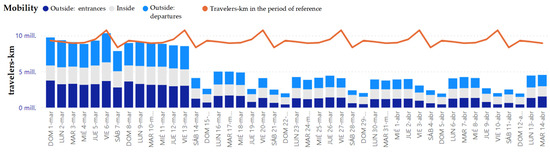
Figure 5.
Evolution of daily mobility using public transport in Cartagena from the entry into force of mobility restrictions in 2020 (in blue) compared to the previous year 2019 (in red). Data source: Ministry of Transport of Spain and Cartagena City Council.
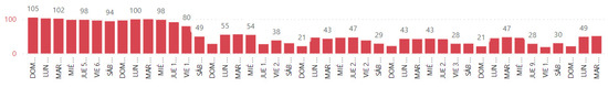
Figure 6.
Percentage of daily mobility using public transport in Cartagena in March and April 2020 compared to the same days in 2019. Data source: Ministry of Transport of Spain and Cartagena City Council.
With the partial return to normality and the relaxation of mobility restrictions brought about by the appearance of vaccines, the figures for the reduction of trips and use of transport in the initial months of the pandemic have been progressively nuanced in the city of Cartagena. In Figure 7 and Figure 8 we can see how up to 70–75% of the pre-pandemic values had recovered globally in the months of March and April 2021.
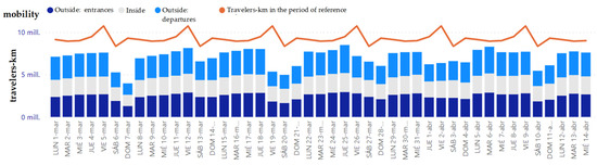
Figure 7.
Evolution of daily mobility using public transport in Cartagena in March and April 2021 (in blue) compared to 2019 (in red). Data source: Ministry of Transport of Spain and Cartagena City Council.
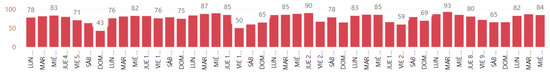
Figure 8.
Percentage of daily mobility using public transport in Cartagena in March and April 2021 compared to the same days in 2019. Data source: Ministry of Transport of Spain and Cartagena City Council.
3.2. Spatial Analysis of the Change of Urban Mobility Patterns during the Pandemic
If these aggregated data for the years 2019, 2020, and 2021 are spatially analyzed in the sectors described, the behavior patterns of the modal split are rather interesting. In the months of March and April of the aforementioned years, the relative weight in urban mobility as a whole has been analyzed for each of the mobility alternatives proposed in the GIS indicators (private transport, public transport, and bicycle/pedestrian travel). The results of the evolution of this relative weight can be seen in Figure 9, Figure 10 and Figure 11 below.
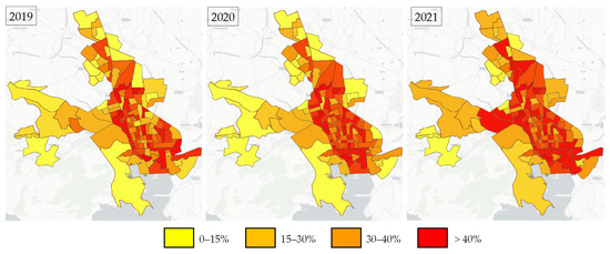
Figure 9.
Evolution of the relative weight of the PVUD indicator in the city’s sectors in the months of March and April of 2019, 2020, and 2021.
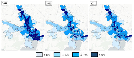
Figure 10.
Evolution of the relative weight of the IPTU indicator in the city’s sectors in the months of March and April of 2019, 2020, and 2021.
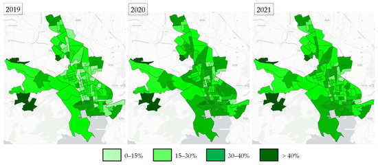
Figure 11.
Evolution of the relative weight of the HMD indicator in the city’s sectors in the months of March and April of 2019, 2020, and 2021.
In the case of the PVUD indicator, it is observed that during the pandemic the presence of private vehicles for accessing the city fell due to the reduction in interurban mobility, but their relative presence in the city center was strengthened due to the need to make essential trips in the urban area, to the detriment of public transport by bus, as confirmed by the IPTU indicator. Public transport suffered a sharp fall, mainly in the urban center during the pandemic in 2020, but unlike the previous case with private transport, it has not recovered to its pre-pandemic status. Only part of the transport in the city center has recovered. Walking and cycling, traditionally more present in low-density peri-urban areas and in the pedestrianized historic center of the city, made up for part of the decline in public transport in many sectors, and in private transport in some areas. However, this has generally returned to pre-pandemic values in the areas of the city where access to private transport has recovered. There is also a greater presence of bike and pedestrian displacements in general, although unable to make up for the sharp drop that still persists in public transport in 2021.
If we analyze these data in an aggregate way for each of the urban mobility alternatives, we can verify that there has been a substantial alteration in the usage patterns of urban mobility during the pandemic. The transfer flows of the modal split obtained through the app-based surveys, the data provided by the public transport concession companies, and the monitoring data of the City Council’s traffic control center are represented in a summarized and schematic way through a Sankey diagram in Figure 12.
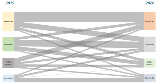
Figure 12.
Simplified Sankey diagram of modal distribution transfer between 2019 and 2020 due to the pandemic.
On the other hand, the behavior of the EAQI parameter of environmental air quality in the city during the pandemic has also been studied at a spatial level. The average values obtained for the months of March and April have been graphed for each of the sectors in the years 2019, 2020, and 2021 in Figure 13.
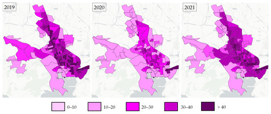
Figure 13.
Evolution of the spatial distribution of the EAQI values in the city’s sectors in the months of March and April of 2019, 2020, and 2021.
Based on the graphs, we can generally see lower pollution values in 2020 than in 2019 due to the pandemic. Following this same criterion, it would seem that, although there is a worsening of air quality in most sectors from 2020 to 2021, there has been a global improvement in the current situation with respect to the pre-pandemic stage. However, this apparently positive situation can be misleading, since traffic levels have not recovered to 2019 levels, and the behavior patterns of mobility have also been modified, as stated in the previous section. Consequently, a spatial statistical study of the correlation between the current trend in the distribution patterns of urban mobility and air quality in the different sectors is carried out to determine to what extent these trends produce positive or negative inertias at the environmental level.
3.3. Spatial Correlation between Changes in Urban Mobility Patterns and Environmental Air Quality Indicators
In the first place, the level of autocorrelation of the spatial indicators is analyzed using the Global Moran I statistic. The observed clustering values indicate that the spatial distribution patterns of urban mobility and air quality do not pose a statistical random behavior (see Table 1).

Table 1.
Global Moran’s I statistic for urban mobility and air quality indicators before and during the COVID-19 pandemic (data order: 2019/2020/2021).
Next, the level of bivariate statistical correlation existing from a spatial point of view between the distribution pattern of each of the modal mobility indicators and the level of air quality has been analyzed using Anselin’s Local Moran’s I statistic (see Table 2). This analysis has been complemented in an aggregate way with a numerical OLS analysis and with a spatial analysis of hot spots with the Getis-Ord Gi * statistic to understand, in a two-dimensional way, the patterns of clustering behavior and the outliers of the existing relationship between the different modal alternatives for mobility and environmental pollution in the city (see Table 3 and Figure 14).
Table 2.
Bivariate Global Moran’s I statistics for spatial correlation between mobility indicators and EQI index (data order: 2019/2020/2021).
Table 3.
Detailed multiple regression models (OLS) for LISA bidimensional analysis of the different levels of air quality index.
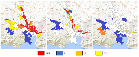
Figure 14.
Current trend of LISA hot spots maps between mobility indicators and AQI for March and April 2021 (case order: PVUD-EAQI/IPTU-EAQI/HMD-EAQI).
Based on the results, we can verify that there is a clear spatial correlation between the areas with the greatest increases in private vehicles and the areas of consolidation with a high level of environmental pollution. This is verified both at the numerical aggregate level in the analysis and in the spatial distribution of the behavior patterns of the modal alternatives linked to the private vehicle (HH cases in Figure 14). We also note that the increase in walking and cycling due to the pandemic is not enough to compensate for the increase in the level of pollution derived from the decline of public transport in most sectors. In any case, as shown by the numerical analysis of the Akaike’s in-formation criterion and the adjusted R2 value, the model behaves better in extreme situations (e.g., high or very low values of pollution levels in 2020) but is less reliable and robust in intermediate or transitional situations, such as in 2021, so these results cannot be taken as definitive.
4. Discussion
The results obtained reflect a more complex reality than that currently inferred on many occasions in relation to the effects of the pandemic in the context of urban mobility in cities, and consequently of the environmental impact of this phenomenon. It is evident that the general paralysis of economic activity, as a result of the inability of developed countries to cope with the spread of the SARS-CoV-2 virus during the first months after the declaration of the worldwide pandemic situation, led to a planet-wide reduction in greenhouse gas emissions, as confirmed by numerous studies [40,41,42,43].
In the case of transport, the reduction of its environmental impact has been prolonged over time in various sectors because of restrictions being maintained on international mobility between countries, as has happened, for example, in the sector of international aviation (which represents one of the most polluting means of transport). However, in the case of urban mobility, this analysis is more complex. The tougher restrictions on mobility in the initial phase of the pandemic led to a reduction in all trips in all modes of transport in cities [44,45], contributing to a global reduction in pollution in these areas, which usually represents a significant percentage (>70%) of all greenhouse gas emissions from transport [20,46]. However, once this initial stage of confusion in the face of the virus that forced administrations to resort to more drastic measures had been overcome, the subsequent re-establishment of the usual activity of the cities has opened a new scenario that is possibly less favorable to the environment [47].
In the case study presented in this work, maintaining certain mobility limitations, such as capacity restrictions in public transport, has led to an inevitable loss of modal share in the distribution of urban mobility alternatives, assuming a clear decrease in several of the most efficient alternatives at an environmental level, as pointed out in other recent case studies [48,49]. On the other hand, an increase in the use of private vehicles in municipal gauges once restrictions on mobility were relaxed has been found in the city of Cartagena. This growth is partially fueled by those users who have abandoned public transport due to the capacity restrictions imposed in this modality, but also by the changes in the behavioral habits of the users because of the psychological effect generated by the risk of contagion of the virus, as some authors point out in other cities [47]. This last pattern of behavior can be corroborated by the reduction in car-sharing systems, which have also experienced a reduction in use compared to private vehicles, as confirmed by the municipal capacity monitoring cameras and the surveys carried out.
The changes in the behavioral patterns of urban mobility are clearly confirmed by the spatial patterns of environmental impact in the different areas of the city where that type of behavior can be seen more clearly reflected (main entrances and points of high traffic concentration). This therefore reflects a dual situation in which, after an initial phase of general reduction in mobility and thus its environmental impacts [43], the effects of the pandemic did not result in a reduction in greenhouse gases, but rather a change of the behavioral patterns of urban mobility that favors a trend of higher environmental impact (but still not higher in total numbers) than the one that existed before the pandemic.
The spatial analysis developed using a spatial statistical approach has therefore been very suitable to carry out an evaluation of this problem in order to go beyond the study of the primary effects of the pandemic on issues such as urban mobility or greenhouse gas emissions. We are therefore facing a secondary effect that is not always easy to determine, as it is partially masked in the traditional aggregated statistical analyses by variables that do in fact maintain a behavior aimed at reducing greenhouse gases due to the absence of mobility in some activities.
It must be borne in mind that in this same initial post-shock period, after which mobility prior to the pandemic has partially recovered [49], several sectors that traditionally generate relevant urban mobility, such as universities or certain business activities, have continued to transfer their daily activity to the field of teleworking [41,50]. This has possibly had a beneficial effect on the reduction of trips, masking some environmental issues and not allowing us to clearly observe the effect of changes in the behavior patterns of other sectors of urban mobility.
However, it is important to analyze in detail these changes in the behavioral patterns of mobility, since, according to the spatial statistical correlation trends analyzed for this case, these changes may be producing a return of more negative characteristics in terms of sustainable mobility than the pre-COVID-19 scenario in which the use of private vehicles has been strengthened compared to public transport. The mitigating elements of the existing reality in 2021 will gradually disappear, whilst some changes in the habitual conduct of mobility users may nevertheless have been negatively consolidated.
The study presented therefore proposes an analysis of a scenario which will require vigilance, as other authors highlight in different studies [21,51,52]. Although it does not represent more than a field of research still in its initial phase (given that the definitive consequences and more permanent scenarios of post-COVID-19 society are not yet consolidated and there is still a long way to go until the pre-pandemic situation is fully recovered), it does reveal a phenomenon that needs to be monitored and analyzed to prevent it from degenerating into undesirable trends in urban and environmental planning in cities.
It must be noted that this study has addressed the existence of other possible sources of urban pollution distorting results. In the meteorological field, the values for the periods of May and April were analyzed for the three years indicated, without there having been any extreme meteorological event that could distort the average values of each of the years (in the case of Cartagena, the only relevant climatological event at the level of measurement of the AQI indicator is a Saharan dust phenomenon from North Africa called ‘calima’ generating high PM10 rates, which in this case did not occur during the months of April and May in any of the last three years). Regarding the wind values, it should be remarked that, in the case of Cartagena, these are fairly stable winds in terms of frequency and direction. Therefore, it can be assumed that the mean temperature, rainfall, and wind speed did not generate any statistically significant bias in the measurements analyzed during these last three years for the period analyzed.
Even so, the analysis carried out has certain clear limitations, since the case evaluated does not represent more than an isolated example and only evaluates a short period of time. It is important to contrast whether it is therefore a consolidated trend or a conjunctural process, so we would need to confirm the current trend in the coming years. The methodology also suffers from some limitations since actual air quality data were obtained at meteorological stations, their distribution across sectors by numerical interpolation of values depending on the distance to the geometric center of the sector (inverse distance method) is possibly not the best solution, since the influence of spatial parameters of buildings is not considered. Therefore, this approach must incorporate future methodological improvements to improve it and make it more statistically robust in the future.
In addition, the case study addressed corresponds to a medium-sized city whose size simplifies the number of variables to consider, thereby reducing the complexity of the analysis, as several authors corroborate for these kind of analysis of urban mobility [22,44,45,53]. Therefore, this does not allow the results to be directly extrapolated to the characteristics of cities with larger populations and sizes, where the trends may have been different, due to the existence of a greater number of variables to analyze in the field of urban mobility.
However, the work carried out does allow an initial research framework to be established with a view to addressing future lines of study involving more sophisticated methodologies based on the positive results obtained through the proposed approach. The existence of results similar to those found in other studies of larger cities on issues such as the drop in the modal share of public transport or the initial reduction in emissions as a consequence of the global reduction in mobility [54,55,56] can lead us to deduce that similar parameters could occur in larger cities.
5. Conclusions
The study carried out shows how the COVID-19 pandemic has affected behavioral patterns of urban mobility in Cartagena (Spain), redistributing the relative weight of each of the mobility alternatives in the city. Although the restrictions imposed by the administrations due to the pandemic initially led to a global reduction in mobility, thus contributing to the reduction of pollution indicators in the city, this study carried out on current trends shows a different inertia. A greater use of private vehicles is consolidated compared to public transport, which does not seem to be compensated by a certain recovery of more sustainable mobility alternatives, such as pedestrian movements and bicycles. These change in behavioral patterns of urban mobility may be temporary or may be consolidated in the coming years, so they should be monitored in the future to address possible effects of the pandemic on the environmental quality of cities.
Author Contributions
Conceptualization, S.G.-A.; methodology, S.G.-A. and P.K.; validation, S.G.-A. and P.K.; formal analysis, S.G.-A. and P.K.; resources, S.G.-A.; data curation, S.G.-A.; writing—original draft preparation, S.G.-A. and P.K.; supervision, S.G.-A. and P.K. All authors have read and agreed to the published version of the manuscript.
Funding
This research received no external funding.
Acknowledgments
The authors acknowledge the collaboration and the data provided by the local authorities of the city of Cartagena to carry out this research.
Conflicts of Interest
The authors declare no conflict of interest.
Appendix A
- Input data of the analysis:
- Urban area analyzed: 17.8 km2/Population: 216,000 inhabitants
- Number of sectors: 135/Bus lines: 32/Bus stops: 425/traffic gauging points: 228
- Number of app surveys: 6345 (2019); 5823 (2020); 3549 (2021, until October).
- Data source for air quality measurements (only regional ones): https://sinqlair.carm.es/calidadaire/ (accessed on 4 November 2021).
References
- Zhang, H.; Ji, Y.; Wu, Z.; Peng, L.; Bao, J.; Peng, Z.; Li, H. Atmospheric volatile halogenated hydrocarbons in air pollution episodes in an urban area of Beijing: Characterization, health risk assessment and sources apportionment. Sci. Total Environ. 2022, 806, 150283. [Google Scholar] [CrossRef]
- Renzi, M.; Marchetti, S.; de’ Donato, F.; Pappagallo, M.; Scortichini, M.; Davoli, M.; Frova, L.; Michelozzi, P.; Stafoggia, M. Acute Effects of Particulate Matter on All-Cause Mortality in Urban, Rural, and Suburban Areas, Italy. Int. J. Environ. Res. Public Heal. 2021, 18, 12895. [Google Scholar] [CrossRef]
- Gustafsson, M.; Svensson, N.; Eklund, M.; Dahl Öberg, J.; Vehabovic, A. Well-to-wheel greenhouse gas emissions of heavy-duty transports: Influence of electricity carbon intensity. Transp. Res. Part D Transp. Environ. 2021, 93, 102757. [Google Scholar] [CrossRef]
- Deenapanray, P.N.K.; Khadun, N.A. Land transport greenhouse gas mitigation scenarios for Mauritius based on modelling transport demand. Transp. Res. Interdiscip. Perspect. 2021, 9, 100299. [Google Scholar] [CrossRef]
- Abarca-Alvarez, F.J.; Navarro-Ligero, M.L.; Valenzuela-Montes, L.M.; Campos-Sánchez, F.S. European Strategies for Adaptation to Climate Change with the Mayors Adapt Initiative by Self-Organizing Maps. Appl. Sci. 2019, 9, 3859. [Google Scholar] [CrossRef] [Green Version]
- Zhou, Y.; Han, J.; Li, J.; Zhou, Y.; Wang, K.; Huang, Y. Building resilient cities with stringent pollution controls: A case study of robust planning of Shenzhen City’s urban agriculture system. J. Clean. Prod. 2021, 311, 127452. [Google Scholar] [CrossRef]
- Yin, H.; Islam, M.S.; Ju, M. Urban river pollution in the densely populated city of Dhaka, Bangladesh: Big picture and rehabilitation experience from other developing countries. J. Clean. Prod. 2021, 321, 129040. [Google Scholar] [CrossRef]
- Millán-Martínez, M.; Sánchez-Rodas, D.; Sánchez de la Campa, A.M.; de la Rosa, J. Contribution of anthropogenic and natural sources in PM10 during North African dust events in Southern Europe. Environ. Pollut. 2021, 290, 118065. [Google Scholar] [CrossRef]
- Guo, L.; Luo, J.; Yuan, M.; Huang, Y.; Shen, H.; Li, T. The influence of urban planning factors on PM2.5 pollution exposure and implications: A case study in China based on remote sensing, LBS, and GIS data. Sci. Total Environ. 2019, 659, 1585–1596. [Google Scholar] [CrossRef]
- Castells-Quintana, D.; Dienesch, E.; Krause, M. Air pollution in an urban world: A global view on density, cities and emissions. Ecol. Econ. 2021, 189, 107153. [Google Scholar] [CrossRef]
- Bächler, P.; Müller, T.K.; Warth, T.; Yildiz, T.; Dittler, A. Impact of ambient air filters on PM concentration levels at an urban traffic hotspot (Stuttgart, Am Neckartor). Atmos. Pollut. Res. 2021, 12, 101059. [Google Scholar] [CrossRef]
- Meng, M.-R.; Cao, S.-J.; Kumar, P.; Tang, X.; Feng, Z. Spatial distribution characteristics of PM2.5 concentration around residential buildings in urban traffic-intensive areas: From the perspectives of health and safety. Saf. Sci. 2021, 141, 105318. [Google Scholar] [CrossRef]
- Fachinger, F.; Drewnick, F.; Borrmann, S. How villages contribute to their local air quality—The influence of traffic- and biomass combustion-related emissions assessed by mobile mappings of PM and its components. Atmos. Environ. 2021, 263, 118648. [Google Scholar] [CrossRef]
- Luppi, B.; Parisi, F.; Rajagopalan, S. The rise and fall of the polluter-pays principle in developing countries. Int. Rev. Law Econ. 2012, 32, 135–144. [Google Scholar] [CrossRef] [Green Version]
- Loorbach, D.; Schwanen, T.; Doody, B.J.; Arnfalk, P.; Langeland, O.; Farstad, E. Transition governance for just, sustainable urban mobility: An experimental approach from Rotterdam, the Netherlands. J. Urban Mobil. 2021, 1, 100009. [Google Scholar] [CrossRef]
- Tenailleau, Q.M.; Tannier, C.; Vuidel, G.; Tissandier, P.; Bernard, N. Assessing the impact of telework enhancing policies for reducing car emissions: Exploring calculation methods for data-missing urban areas—Example of a medium-sized European city (Besançon, France). Urban Clim. 2021, 38, 100876. [Google Scholar] [CrossRef]
- Campos-Sánchez, F.S.; Valenzuela-Montes, L.M.; Abarca-Álvarez, F.J. Evidence of Green Areas, Cycle Infrastructure and Attractive Destinations Working Together in Development on Urban Cycling. Sustainability 2019, 11, 4730. [Google Scholar] [CrossRef] [Green Version]
- Sharmilaa, G.; Ilango, T. Vehicular air pollution based on traffic density—A case study. Mater. Today Proc. 2021. [Google Scholar] [CrossRef]
- Kazancoglu, Y.; Ozbiltekin-Pala, M.; Ozkan-Ozen, Y.D. Prediction and evaluation of greenhouse gas emissions for sustainable road transport within Europe. Sustain. Cities Soc. 2021, 70, 102924. [Google Scholar] [CrossRef]
- Quintyne, K.I.; Kelly, C.; Sheridan, A.; Kenny, P.; O’Dwyer, M. COVID-19 transport restrictions in Ireland: Impact on air quality and respiratory hospital admissions. Public Health 2021, 198, 156–160. [Google Scholar] [CrossRef]
- Wimbadi, R.W.; Djalante, R.; Mori, A. Urban experiments with public transport for low carbon mobility transitions in cities: A systematic literature review (1990–2020). Sustain. Cities Soc. 2021, 72, 103023. [Google Scholar] [CrossRef]
- Gonzalez, J.N.; Perez-Doval, J.; Gomez, J.; Vassallo, J.M. What impact do private vehicle restrictions in urban areas have on car ownership? Empirical evidence from the city of Madrid. Cities 2021, 116, 103301. [Google Scholar] [CrossRef]
- De Oña, J.; Estévez, E.; de Oña, R. Public transport users versus private vehicle users: Differences about quality of service, satisfaction and attitudes toward public transport in Madrid (Spain). Travel Behav. Soc. 2021, 23, 76–85. [Google Scholar] [CrossRef]
- Gomez, J.; Aguilera-García, Á.; Dias, F.F.; Bhat, C.R.; Vassallo, J.M. Adoption and frequency of use of ride-hailing services in a European city: The case of Madrid. Transp. Res. Part C Emerg. Technol. 2021, 131, 103359. [Google Scholar] [CrossRef]
- Sánchez-Barroso, G.; González-Domínguez, J.; García-Sanz-Calcedo, J.; Sokol, M. Impact of weather-influenced urban mobility on carbon footprint of Spanish healthcare centres. J. Transp. Heal. 2021, 20, 101017. [Google Scholar] [CrossRef]
- Muñiz, I.; Sánchez, V. Urban Spatial Form and Structure and Greenhouse-gas Emissions From Commuting in the Metropolitan Zone of Mexico Valley. Ecol. Econ. 2018, 147, 353–364. [Google Scholar] [CrossRef]
- Fernández, R.Á.; Caraballo, S.C.; López, F.C. A probabilistic approach for determining the influence of urban traffic management policies on energy consumption and greenhouse gas emissions from a battery electric vehicle. J. Clean. Prod. 2019, 236, 117604. [Google Scholar] [CrossRef]
- Ribeiro, F.N.D.; Umezaki, A.S.; Chiquetto, J.B.; Santos, I.; Machado, P.G.; Miranda, R.M.; Almeida, P.S.; Simões, A.F.; Mouette, D.; Leichsenring, A.R.; et al. Impact of different transportation planning scenarios on air pollutants, greenhouse gases and heat emission abatement. Sci. Total Environ. 2021, 781, 146708. [Google Scholar] [CrossRef]
- Regmi, M.B. Measuring sustainability of urban mobility: A pilot study of Asian cities. Case Stud. Transp. Policy 2020, 8, 1224–1232. [Google Scholar] [CrossRef]
- Silva, B.V.F.; Teles, M.P.R. Pathways to sustainable urban mobility planning: A case study applied in São Luís, Brazil. Transp. Res. Interdiscip. Perspect. 2020, 4, 100102. [Google Scholar] [CrossRef]
- García-Ayllón, S. Retro-diagnosis methodology for land consumption analysis towards sustainable future scenarios: Application to a mediterranean coastal area. J. Clean. Prod. 2018, 195, 1408–1421. [Google Scholar] [CrossRef]
- De Miguel Molina, M.; De Miguel Molina, B.; Catalá Pérez, D.; Santamarina Campos, V. Connecting passenger loyalty to preferences in the urban passenger transport: Trends from an empirical study of taxi vs. VTC services in Spain. Res. Transp. Bus. Manag. 2021, 100661. [Google Scholar] [CrossRef]
- de Oña, J. The role of involvement with public transport in the relationship between service quality, satisfaction and behavioral intentions. Transp. Res. Part A Policy Pract. 2020, 142, 296–318. [Google Scholar] [CrossRef]
- de Oña, J.; Estévez, E.; de Oña, R. How does private vehicle users perceive the public transport service quality in large metropolitan areas? A European comparison. Transp. Policy 2021, 112, 173–188. [Google Scholar] [CrossRef]
- Garcia-Ayllon, S.; Hontoria, E.; Munier, N. The Contribution of MCDM to SUMP: The Case of Spanish Cities during 2006-2021. Int. J. Environ. Res. Public Heal. 2022, 19, 294. [Google Scholar] [CrossRef]
- European Commission Directive 2008/50/EC of the European Parliament and of the Council of 21 May 2008 on ambient air quality and cleaner air for Europe. Off. J. Eur. Union 2008, 152, 1–44.
- Wu, C. Handbook of Applied Spatial Analysis: Software Tools, Methods and Applications edited by Manfred, M. Fischer and Arthur Getis. J. Reg. Sci. 2012, 52, 386–388. [Google Scholar] [CrossRef]
- Ding, Y.; Fotheringham, A.S. The integration of spatial analysis and gis. Comput. Environ. Urban Syst. 1992, 16, 3–19. [Google Scholar] [CrossRef] [Green Version]
- Anselin, L. Local Indicators of Spatial Association—LISA. Geogr. Anal. 1995, 27, 93–115. [Google Scholar] [CrossRef]
- Singh, V.; Mishra, V. Environmental impacts of coronavirus disease 2019 (COVID-19). Bioresour. Technol. Reports 2021, 15, 100744. [Google Scholar] [CrossRef] [PubMed]
- Perkins, K.M.; Munguia, N.; Ellenbecker, M.; Moure-Eraso, R.; Velazquez, L. COVID-19 pandemic lessons to facilitate future engagement in the global climate crisis. J. Clean. Prod. 2021, 290, 125178. [Google Scholar] [CrossRef] [PubMed]
- Kumar, A.; Singh, P.; Raizada, P.; Hussain, C.M. Impact of COVID-19 on greenhouse gases emissions: A critical review. Sci. Total Environ. 2022, 806, 150349. [Google Scholar] [CrossRef] [PubMed]
- Abubakar, L.; Salemcity, A.J.; Abass, O.K.; Olajuyin, A.M. The impacts of COVID-19 on environmental sustainability: A brief study in world context. Bioresour. Technol. Reports 2021, 15, 100713. [Google Scholar] [CrossRef]
- Bazzana, D.; Cohen, J.J.; Golinucci, N.; Hafner, M.; Noussan, M.; Reichl, J.; Rocco, M.V.; Sciullo, A.; Vergalli, S. A multi-disciplinary approach to estimate the medium-term impact of COVID-19 on transport and energy: A case study for Italy. Energy 2022, 238, 122015. [Google Scholar] [CrossRef]
- Zhang, R.; Zhang, J. Long-term pathways to deep decarbonization of the transport sector in the post-COVID world. Transp. Policy 2021, 110, 28–36. [Google Scholar] [CrossRef]
- Cződörová, R.; Dočkalik, M.; Gnap, J. Impact of COVID-19 on bus and urban public transport in SR. Transp. Res. Procedia 2021, 55, 418–425. [Google Scholar] [CrossRef]
- Echaniz, E.; Rodríguez, A.; Cordera, R.; Benavente, J.; Alonso, B.; Sañudo, R. Behavioural changes in transport and future repercussions of the COVID-19 outbreak in Spain. Transp. Policy 2021, 111, 38–52. [Google Scholar] [CrossRef]
- Nguyen, M.H.; Pojani, D. Covid-19 need not spell the death of public transport: Learning from Hanoi’s safety measures. J. Transp. Heal. 2021, 23, 101279. [Google Scholar] [CrossRef] [PubMed]
- Beck, M.J.; Hensher, D.A.; Nelson, J.D. Public transport trends in Australia during the COVID-19 pandemic: An investigation of the influence of bio-security concerns on trip behaviour. J. Transp. Geogr. 2021, 96, 103167. [Google Scholar] [CrossRef] [PubMed]
- Spadaro, I.; Pirlone, F. Sustainable Urban Mobility Plan and Health Security. Sustainability 2021, 13, 4403. [Google Scholar] [CrossRef]
- Askarizad, R.; Jinliao, H.; Jafari, S. The influence of COVID-19 on the societal mobility of urban spaces. Cities 2021, 119, 103388. [Google Scholar] [CrossRef]
- Kesselring, S.; Freudendal-Pedersen, M. Searching for urban mobilities futures. Methodological innovation in the light of COVID-19. Sustain. Cities Soc. 2021, 75, 103138. [Google Scholar] [CrossRef]
- Romero, F.; Gomez, J.; Rangel, T.; Vassallo, J.M. Impact of restrictions to tackle high pollution episodes in Madrid: Modal share change in commuting corridors. Transp. Res. Part D Transp. Environ. 2019, 77, 77–91. [Google Scholar] [CrossRef]
- Abdullah, M.; Ali, N.; Javid, M.A.; Dias, C.; Campisi, T. Public transport versus solo travel mode choices during the COVID-19 pandemic: Self-reported evidence from a developing country. Transp. Eng. 2021, 5, 100078. [Google Scholar] [CrossRef]
- Vickerman, R. Will Covid-19 put the public back in public transport? A UK perspective. Transp. Policy 2021, 103, 95–102. [Google Scholar] [CrossRef] [PubMed]
- Lin, N.; Du, W.; Wang, J.; Yun, X.; Chen, L. The effect of COVID-19 restrictions on particulate matter on different modes of transport in China. Environ. Res. 2021, 112205. [Google Scholar] [CrossRef] [PubMed]
Publisher’s Note: MDPI stays neutral with regard to jurisdictional claims in published maps and institutional affiliations. |
© 2022 by the authors. Licensee MDPI, Basel, Switzerland. This article is an open access article distributed under the terms and conditions of the Creative Commons Attribution (CC BY) license (https://creativecommons.org/licenses/by/4.0/).