
Effects of Cropland Expansion on Temperature Extremes in Western India from 1982 to 2015


Abstract
1. Introduction

2. Materials and Methods
2.1. Materials
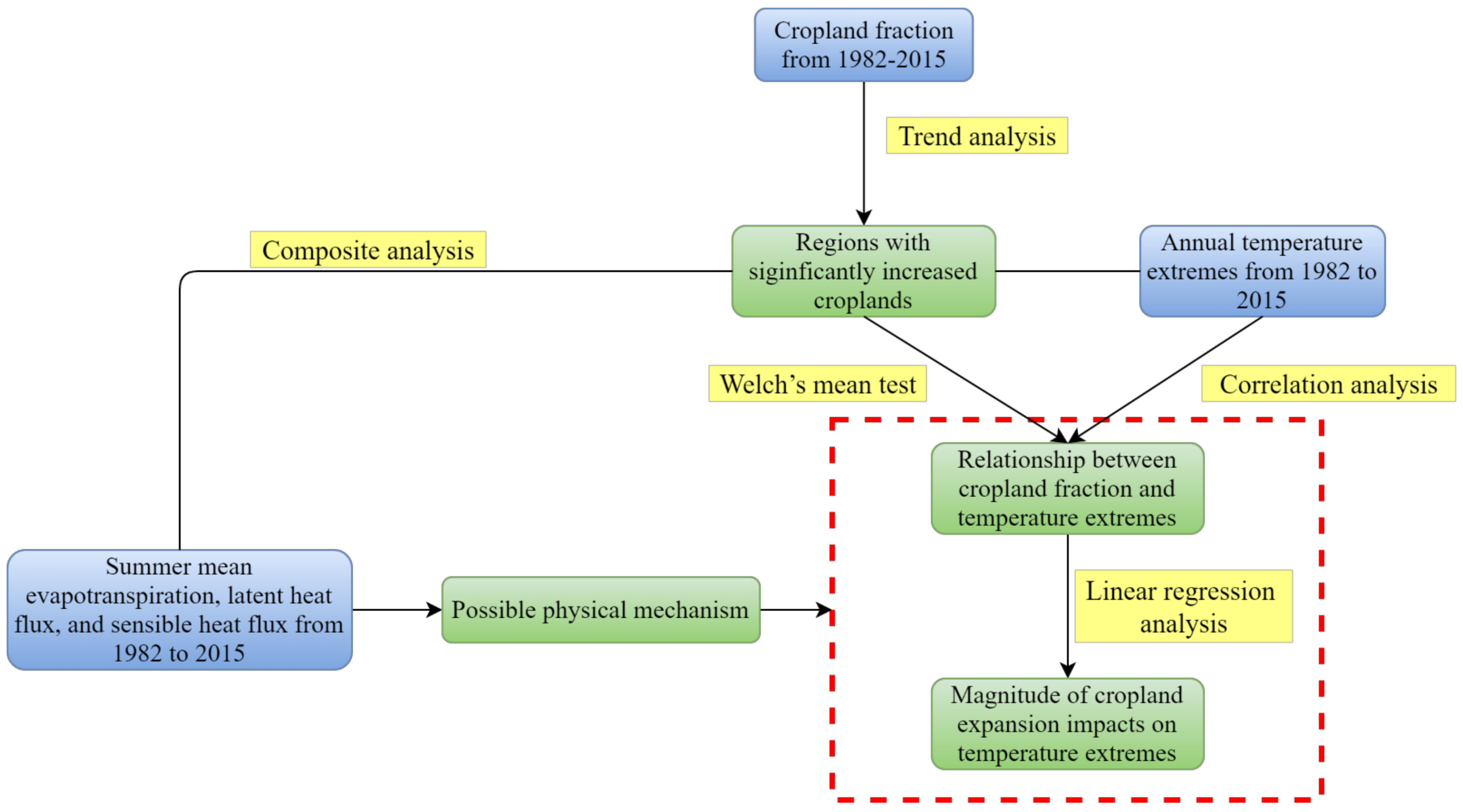
2.2. Methods
2.2.1. Autocorrelation-Adjusted Trend Analysis
2.2.2. Correlation Analysis and Welch’s Mean Test
2.2.3. Linear Regression Analysis
2.2.4. Composite Analysis
3. Results and Discussion
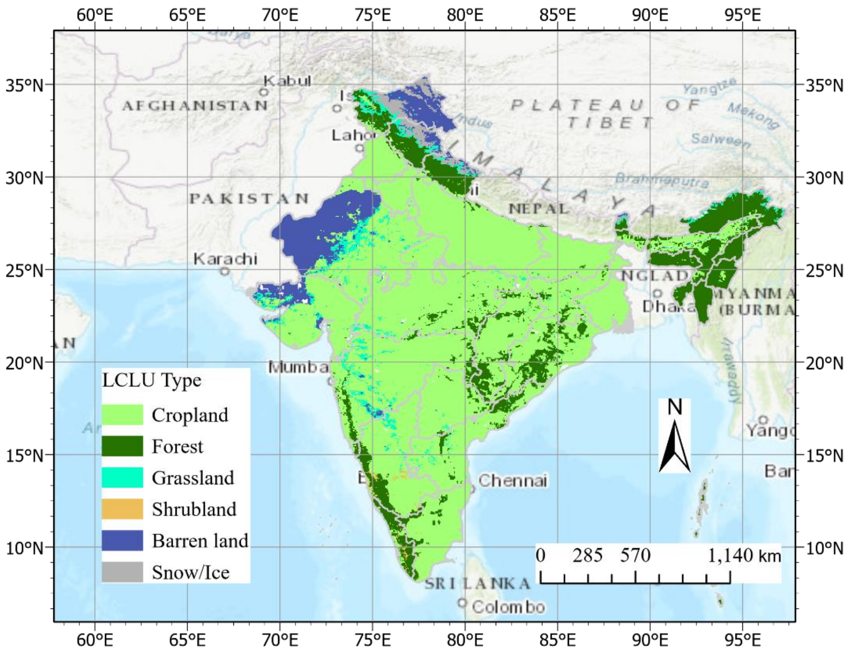
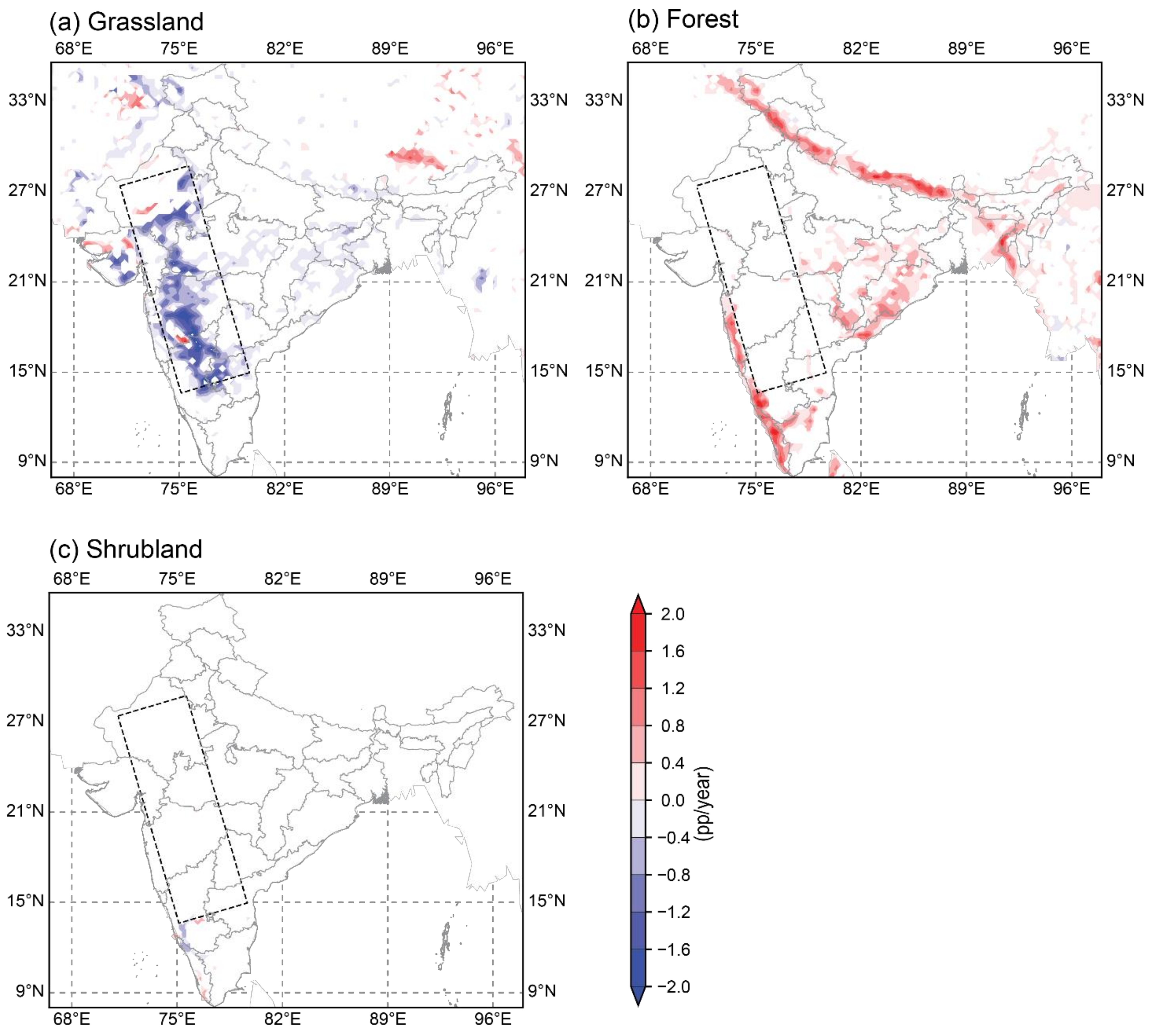
3.1. Cropland Expansion in Western India
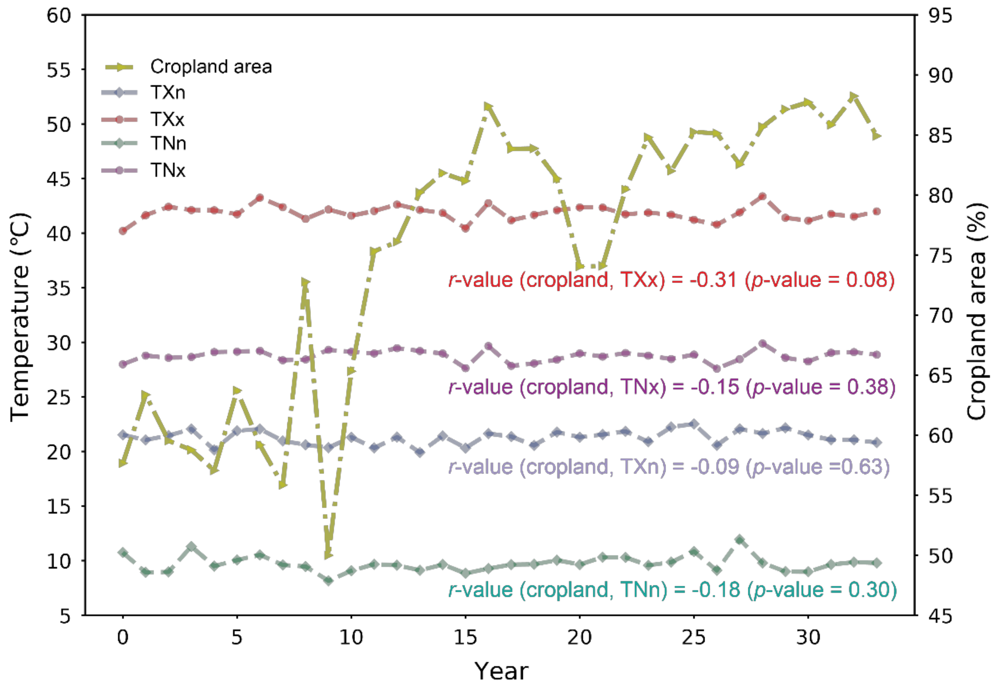
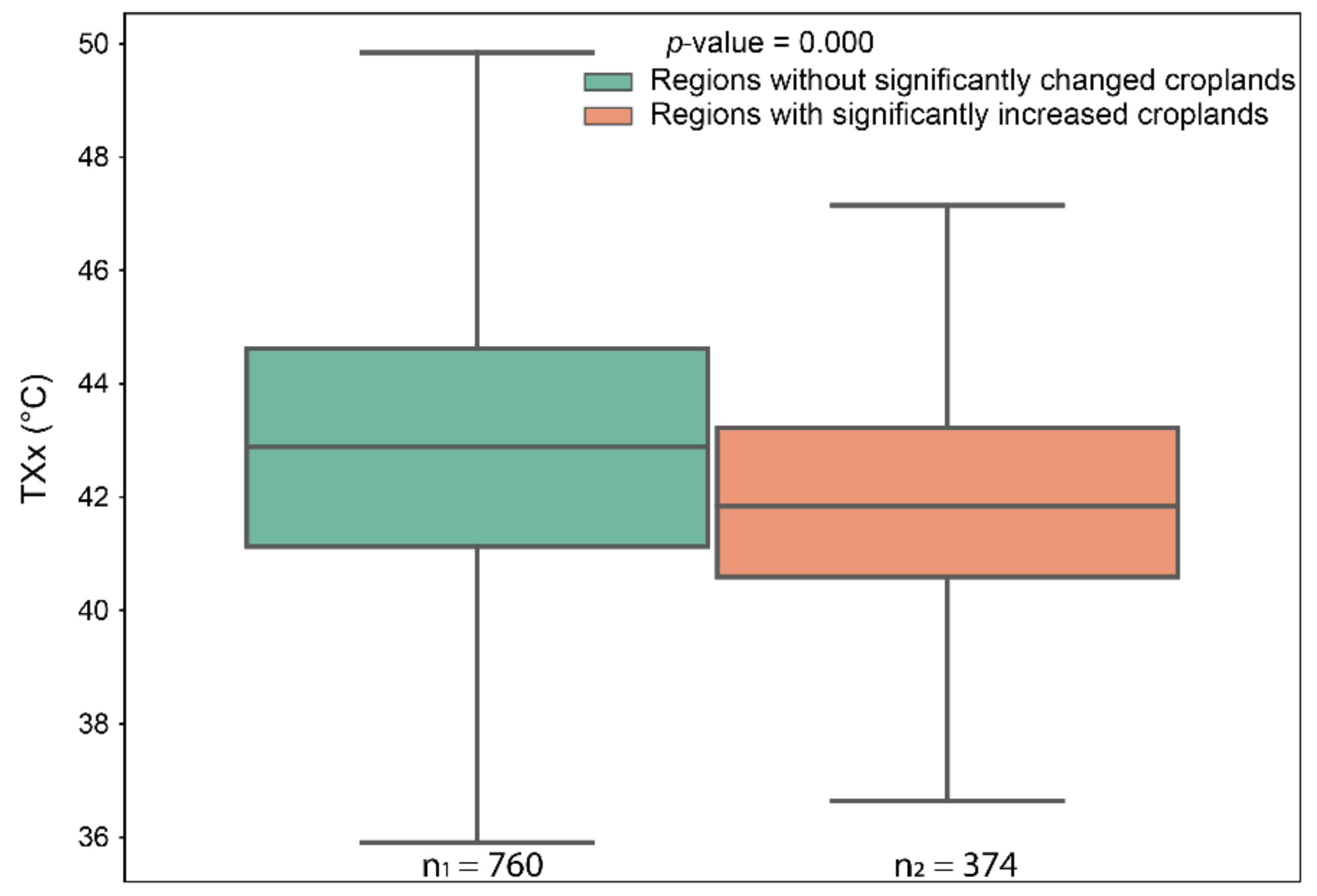
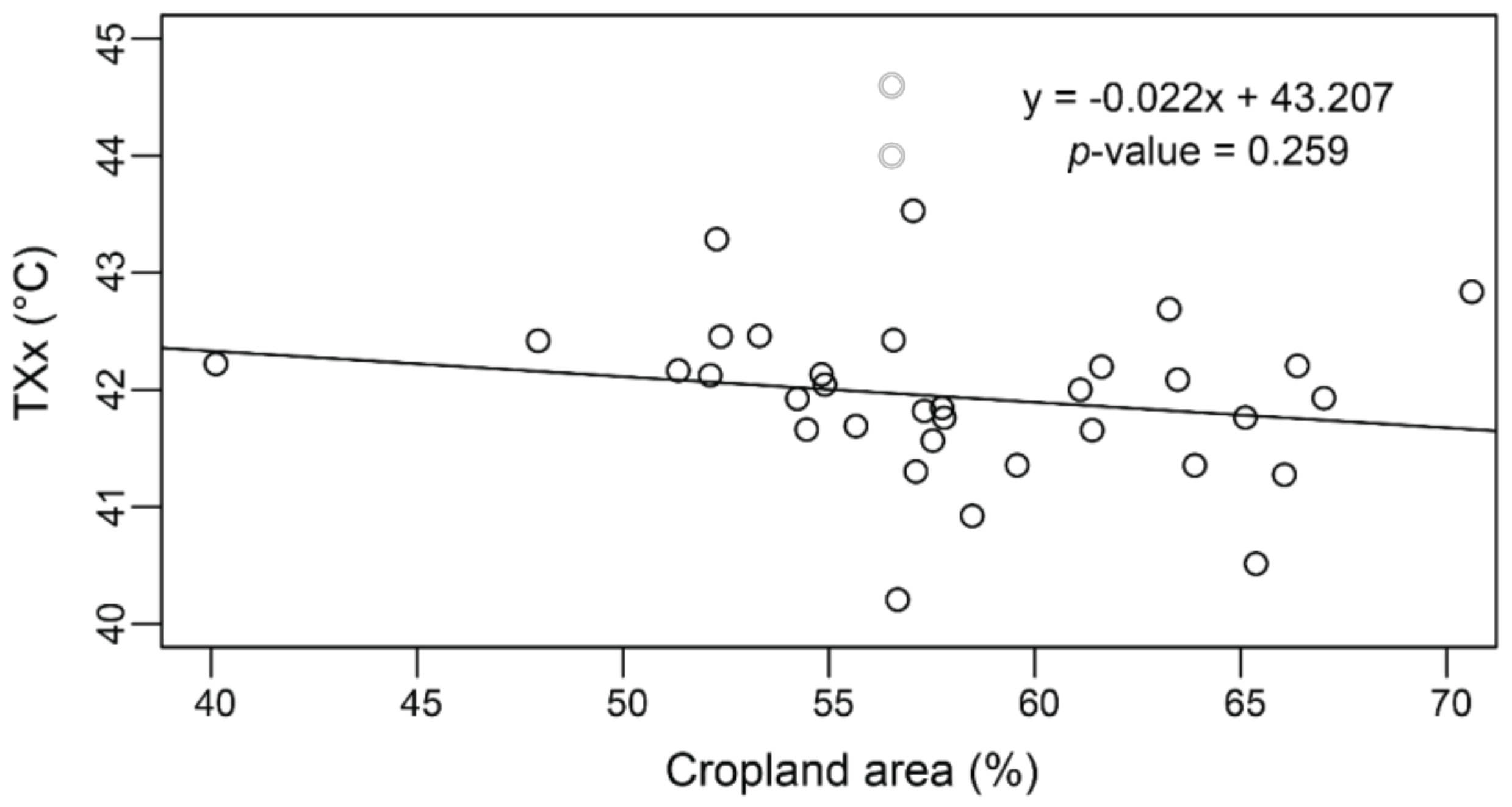
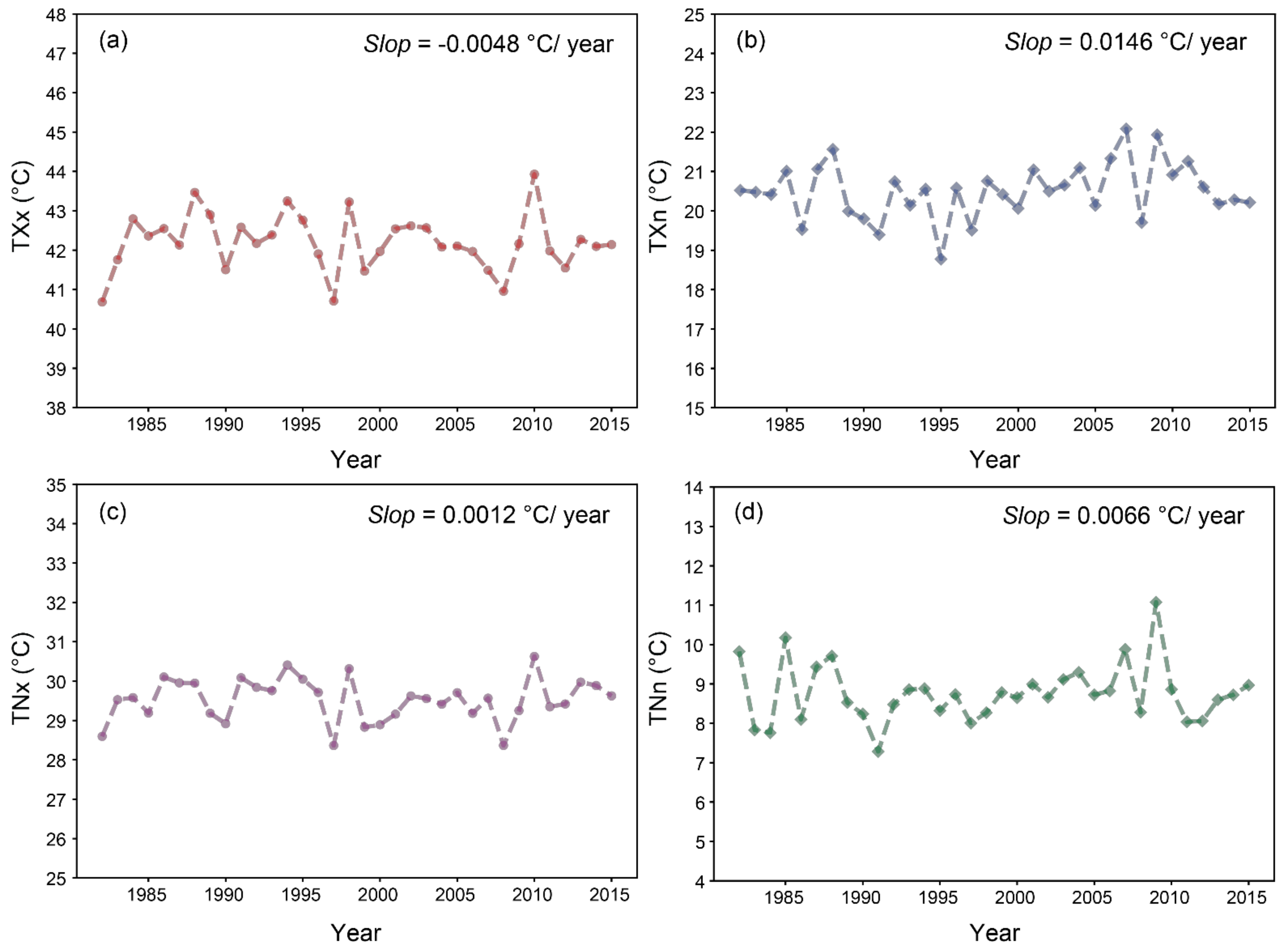
3.2. Impacts of Cropland Expansion on Temperature Extremes in Western India
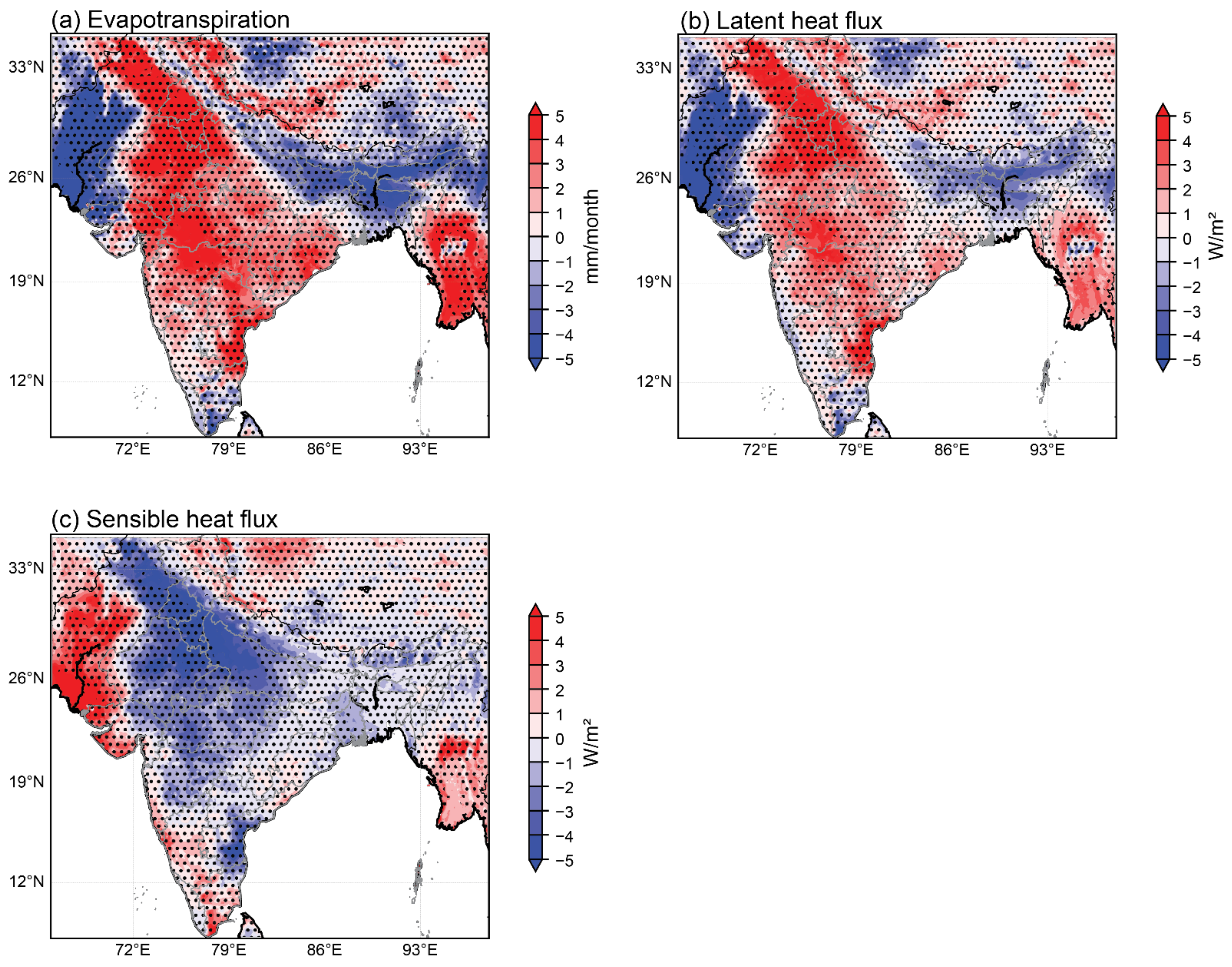
3.3. Possible Physical Mechanisms
4. Conclusions
Author Contributions
Funding
Data Availability Statement
Acknowledgments
Conflicts of Interest
Appendix A


References
- Liu, M.; Xu, X.; Xu, C.; Sun, A.Y.; Wang, K.; Scandon, B.R.; Zhang, L. Water Resources Research: Preface. Water Resour. Res. 2017, 53, 3262–3278. [Google Scholar] [CrossRef]
- Roxy, M.K.; Ghosh, S.; Pathak, A.; Athulya, R.; Mujumdar, M.; Murtugudde, R.; Terray, P.; Rajeevan, M. A threefold rise in widespread extreme rain events over central India. Nat. Commun. 2017, 8, 1–11. [Google Scholar] [CrossRef] [PubMed]
- Kothawale, D.R.; Revadekar, J.V.; Kumar, K.R. Recent trends in pre-monsoon daily temperature extremes over India. J. Earth Syst. Sci. 2010, 119, 51–65. [Google Scholar] [CrossRef]
- Kothawale, D.R.; Rupa Kumar, K. On the recent changes in surface temperature trends over India. Geophys. Res. Lett. 2005, 32, 1–4. [Google Scholar] [CrossRef]
- Chandrashekhar, V. As the Monsoon and Climate Shift, India Faces Worsening Floods. Available online: https://e360.yale.edu/features/as-the-monsoon-and-climate-shift-india-faces-worsening-floods (accessed on 20 October 2020).
- Azhar, G.S.; Mavalankar, D.; Nori-Sarma, A.; Rajiva, A.; Dutta, P.; Jaiswal, A.; Sheffield, P.; Knowlton, K.; Hess, J.J. Heat-related mortality in India: Excess all-cause mortality associated with the 2010 Ahmedabad heat wave. PLoS ONE 2014, 9. [Google Scholar] [CrossRef]
- Times of India. Heat Waves Killed over 6000 since 2010. Available online: https://reliefweb.int/report/india/heat-waves-killed-over-6000-2010#:~:text=NEW%20DELHI%3A (accessed on 12 January 2020).
- Rajsekhar, D.; Gorelick, S.M. Increasing drought in Jordan: Climate change and cascading Syrian land-use impacts on reducing transboundary flow. Sci. Adv. 2017, 3, 1–16. [Google Scholar] [CrossRef]
- Herring, S.C.; Christidis, N.; Hoell, A.; Hoerling, M.P.; Stott, P.A. Explaining extreme events of 2017 from a climate perspective. Bull. Am. Meteorol. Soc. 2019, 100, S1–S117. [Google Scholar] [CrossRef]
- Oueslati, B.; Yiou, P.; Jézéquel, A. Revisiting the dynamic and thermodynamic processes driving the record-breaking January 2014 precipitation in the southern UK. Sci. Rep. 2019, 9, 1–7. [Google Scholar] [CrossRef]
- CarbonBrief Mapped: How Climate Change Affects Extreme Weather around the World. Available online: https://www.carbonbrief.org/mapped-how-climate-change-affects-extreme-weather-around-the-world (accessed on 10 April 2020).
- Lawrence, D.M.; Hurtt, G.C.; Arneth, A.; Brovkin, V.; Calvin, K.V.; Jones, A.D.; Jones, C.D.; Lawrence, P.J.; De Noblet-Ducoudré, N.; Pongratz, J.; et al. The Land Use Model Intercomparison Project (LUMIP) contribution to CMIP6: Rationale and experimental design. Geosci. Model Dev. 2016, 9, 2973–2998. [Google Scholar] [CrossRef]
- Sterling, S.M.; Ducharne, A.; Polcher, J. The impact of global land-cover change on the terrestrial water cycle. Nat. Clim. Chang. 2013, 3, 385–390. [Google Scholar] [CrossRef]
- Thiery, W.; Visser, A.J.; Fischer, E.M.; Hauser, M.; Hirsch, A.L.; Lawrence, D.M.; Lejeune, Q.; Davin, E.L.; Seneviratne, S.I. Warming of hot extremes alleviated by expanding irrigation. Nat. Commun. 2020, 11, 1–7. [Google Scholar] [CrossRef]
- Stoy, P.C. Deforestation intensifies hot days. Nat. Clim. Chang. 2018, 8, 360–369. [Google Scholar] [CrossRef]
- Findell, K.L.; Berg, A.; Gentine, P.; Krasting, J.P.; Lintner, B.R.; Malyshev, S.; Santanello, J.A.; Shevliakova, E. The impact of anthropogenic land use and land cover change on regional climate extremes. Nat. Commun. 2017, 8, 1–9. [Google Scholar] [CrossRef]
- Mueller, N.D.; Rhines, A.; Butler, E.E.; Ray, D.K.; Siebert, S.; Holbrook, N.M.; Huybers, P. Global relationships between cropland intensification and summer temperature extremes over the last 50 years. J. Clim. 2017, 30, 7505–7528. [Google Scholar] [CrossRef]
- He, Y.; Lee, E.; Mankin, S.J. Seasonal tropospheric cooling in Northeast China associated with cropland expansion. Environ. Res. Lett. 2020, 15, 034032. [Google Scholar] [CrossRef]
- Unnikrishnan, C.K.; Gharai, B.; Mohandas, S.; Mamgain, A.; Rajagopal, E.N.; Iyengar, G.R.; Rao, P.V.N. Recent changes on land use/land cover over Indian region and its impact on the weather prediction using Unified model. Atmos. Sci. Lett. 2016, 17, 294–300. [Google Scholar] [CrossRef]
- Halder, S.; Saha, S.K.; Dirmeyer, P.A.; Chase, T.N.; Goswami, B.N. Investigating the impact of land-use land-cover change on Indian summer monsoon daily rainfall and temperature during 1951–2005 using a regional climate model. Hydrol. Earth Syst. Sci. 2016, 20, 1765–1784. [Google Scholar] [CrossRef]
- Li, X.; Mitra, C.; Dong, L.; Yang, Q. Understanding land use change impacts on microclimate using Weather Research and Forecasting (WRF) model. Phys. Chem. Earth 2018, 103, 115–126. [Google Scholar] [CrossRef]
- Gogoi, P.P.; Vinoj, V.; Swain, D.; Roberts, G.; Dash, J.; Tripathy, S. Land use and land cover change effect on surface temperature over Eastern India. Sci. Rep. 2019, 9, 1–10. [Google Scholar] [CrossRef]
- Mukherjee, F.; Singh, D. Assessing Land Use–Land Cover Change and Its Impact on Land Surface Temperature Using LANDSAT Data: A Comparison of Two Urban Areas in India. Earth Syst. Environ. 2020, 4, 385–407. [Google Scholar] [CrossRef]
- Nayak, S.; Mandal, M. Impact of land use and land cover changes on temperature trends over India. Land Use Policy 2019, 89. [Google Scholar] [CrossRef]
- Lee, E.; Chase, T.N.; Rajagopalan, B.; Barry, R.; Biggs, T.; Lawrence, P. Effects of irrigation and vegetation activity on early Indian summer monsoon variability. Int. J. Climatol. 2009, 29, 573–581. [Google Scholar] [CrossRef]
- Paul, S.; Ghosh, S.; Oglesby, R.; Pathak, A.; Chandrasekharan, A.; Ramsankaran, R. Weakening of Indian Summer Monsoon Rainfall due to Changes in Land Use Land Cover. Sci. Rep. 2016, 6, 1–10. [Google Scholar] [CrossRef] [PubMed]
- Chen, L.; Dirmeyer, P.A. The relative importance among anthropogenic forcings of land use/land cover change in affecting temperature extremes. Clim. Dyn. 2019, 52, 2269–2285. [Google Scholar] [CrossRef]
- Kang, S.; Eltahir, E.A.B. North China Plain threatened by deadly heatwaves due to climate change and irrigation. Nat. Commun. 2018, 9, 1–9. [Google Scholar] [CrossRef] [PubMed]
- Sy, S.; Quesada, B. Anthropogenic land cover change impact on climate extremes during the 21st century. Environ. Res. Lett. 2020, 15. [Google Scholar] [CrossRef]
- Christidis, N.; Stott, P.A.; Hegerl, G.C.; Betts, R.A. The role of land use change in the recent warming of daily extreme temperatures. Geophys. Res. Lett. 2013, 40, 589–594. [Google Scholar] [CrossRef]
- Strack, J.E.; Pielke, R.A.; Steyaert, L.T.; Knox, R.G. Sensitivity of June near-surface temperatures and precipitation in the eastern United States to historical land cover changes since European settlement. Water Resour. Res. 2008, 44, 1–13. [Google Scholar] [CrossRef]
- Wang, F.; Notaro, M.; Liu, Z.; Chen, G. Observed local and remote influences of vegetation on the atmosphere across North America using a model-validated statistical technique that first excludes oceanic forcings. J. Clim. 2014, 27, 362–382. [Google Scholar] [CrossRef]
- He, Y.; Warner, T.A.; McNeil, B.E.; Lee, E. Reducing uncertainties in applying remotely sensed land use and land cover maps in land-atmosphere interaction: Identifying change in space and time. Remote Sens. 2018, 10, 506. [Google Scholar] [CrossRef]
- Liu, H.; Gong, P.; Wang, J.; Clinton, N.; Bai, Y.; Liang, S. Annual dynamics of global land cover and its long-term changes from 1982 to 2015. Earth Syst. Sci. Data 2020, 12, 1217–1243. [Google Scholar] [CrossRef]
- Van Etten, J.; Sumner, M.; Cheng, J.; Baston, D.; Bevan, A.; Bivand, R.; Busetto, L.; Canty, M.; Fasoli, B.; Forrest, D.; et al. Package ‘Raster’. Available online: https://cran.r-project.org/web/packages/raster/raster.pdf (accessed on 8 October 2020).
- Hersbach, H.; Bell, B.; Berrisford, P.; Hirahara, S.; Horányi, A.; Muñoz-Sabater, J.; Nicolas, J.; Peubey, C.; Radu, R.; Schepers, D.; et al. The ERA5 global reanalysis. Q. J. R. Meteorol. Soc. 2020, 146, 1999–2049. [Google Scholar] [CrossRef]
- Santer, B.D.; Wigley, T.M.L.; Boyle, J.S.; Gaffen, D.J.; Hnilo, J.J.; Nychka, D.; Parker, D.E.; Taylor, K.E. Statistical significance of trends and trend differences in layer-average atmospheric temperature time series. J. Geophys. Res. Atmos. 2000, 105, 7337–7356. [Google Scholar] [CrossRef]
- Gedney, N.; Valdes, P.J. The effect of Amazonian deforestation on the northern hemisphere circulation and climate. Geophys. Res. Lett. 2000, 27, 3053–3056. [Google Scholar]
- Pal, S.; Ziaul, S. Detection of land use and land cover change and land surface temperature in English Bazar urban centre. Egypt. J. Remote Sens. Sp. Sci. 2017, 20, 125–145. [Google Scholar] [CrossRef]
- Hurley, J.V.; Boos, W.R. Interannual variability of monsoon precipitation and local subcloud equivalent potential temperature. J. Clim. 2013, 26, 9507–9527. [Google Scholar] [CrossRef]
- Ruxton, G.D. The unequal variance t-test is an underused alternative to Student’s t-test and the Mann-Whitney U test. Behav. Ecol. 2006, 17, 688–690. [Google Scholar] [CrossRef]
- Boschat, G.; Simmonds, I.; Purich, A.; Cowan, T.; Pezza, A.B. On the use of composite analyses to form physical hypotheses: An example from heat wave-SST associations. Sci. Rep. 2016, 6, 1–10. [Google Scholar] [CrossRef]
- Roy, P.S.; Roy, A.; Joshi, P.K.; Kale, M.P.; Srivastava, V.K.; Srivastava, S.K.; Dwevidi, R.S.; Joshi, C.; Behera, M.D.; Meiyappan, P.; et al. Development of decadal (1985–1995–2005) land use and land cover database for India. Remote Sens. 2015, 7, 2401–2430. [Google Scholar] [CrossRef]
- Duraisamy, V.; Bendapudi, R.; Jadhav, A. Identifying hotspots in land use land cover change and the drivers in a semi-arid region of India. Environ. Monit. Assess. 2018, 190. [Google Scholar] [CrossRef]
- Tian, H.; Banger, K.; Bo, T.; Dadhwal, V.K. History of land use in India during 1880–2010: Large-scale land transformations reconstructed from satellite data and historical archives. Glob. Planet. Chang. 2014, 121, 78–88. [Google Scholar] [CrossRef]
- Meiyappan, P.; Roy, P.S.; Sharma, Y.; Ramachandran, R.M.; Joshi, P.K.; DeFries, R.S.; Jain, A.K. Dynamics and determinants of land change in India: Integrating satellite data with village socioeconomics. Reg. Environ. Chang. 2017, 17, 753–766. [Google Scholar] [CrossRef]
- Thiery, W.; Davin, E.L.; Lawrence, D.M.; Hirsch, A.L.; Hauser, M.; Seneviratne, S.I. Present-day irrigation mitigates heat extremes. J. Geophys. Res. 2017, 122, 1403–1422. [Google Scholar] [CrossRef]
- Niu, X.; Tang, J.; Wang, S.; Fu, C. Impact of future land use and land cover change on temperature projections over East Asia. Clim. Dyn. 2019, 52, 6475–6490. [Google Scholar] [CrossRef]
- Basha, G.; Kishore, P.; Ratnam, M.V.; Jayaraman, A.; Kouchak, A.A.; Ouarda, T.B.M.J.; Velicogna, I. Historical and Projected Surface Temperature over India during the 20th and 21st century. Sci. Rep. 2017, 7, 1–10. [Google Scholar] [CrossRef]
- Chowdary, J.S.; John, N.; Gnanaseelan, C. Interannual variability of surface air-temperature over India: Impact of ENSO and Indian Ocean Sea surface temperature. Int. J. Climatol. 2014, 34, 416–429. [Google Scholar] [CrossRef]
- Mishra, S.K.; Anand, A.; Fasullo, J.; Bhagat, S. Importance of the resolution of surface topography in Indian monsoon simulation. J. Clim. 2018, 31, 4879–4898. [Google Scholar] [CrossRef]
- Kalsi, S.R.; Pareek, R.S. Hottest April of the 20th century over north-west and central India. Curr. Sci. 2001, 80, 867–873. [Google Scholar]
- Brouwer, C.; Heibloem, M. Irrigation Water Management: Irrigation Water Needs. Available online: http://www.fao.org/3/s2022e/s2022e00.htm#Contents (accessed on 6 July 2020).
- Kumar, M.D.; Sivamohan, M. Pampered Views and Parrot Talks: In the Cause of Well Irrigation in India. In Proceedings of the Sustaining Commons: Sustaining Our Future, the Thirteenth Biennial Conference of the International Association for the Study of the Commons, Hyderabad, India; 2011; pp. 1–24. Available online: https://dlc.dlib.indiana.edu/dlc/bitstream/handle/10535/7270/1205.pdf?sequence=1&isAllowed=y (accessed on 10 January 2021).
- Chen, Y.; Niu, J.; Kang, S.; Zhang, X. Effects of irrigation on water and energy balances in the Heihe River basin using VIC model under different irrigation scenarios. Sci. Total Environ. 2018, 645, 1183–1193. [Google Scholar] [CrossRef] [PubMed]
- Yang, Z.; Dominguez, F.; Zeng, X.; Hu, H.; Gupta, H.; Yang, B. Impact of irrigation over the California Central Valley on regional climate. J. Hydrometeorol. 2017, 18, 1341–1357. [Google Scholar] [CrossRef]
- Ray, D.K.; Nair, U.S.; Welch, R.M.; Han, Q.; Zeng, J.; Su, W.; Kikuchi, T.; Lyons, T.J. Effects of land use in Southwest Australia: 1. Observations of cumulus cloudiness and energy fluxes. J. Geophys. Res. Atmos. 2003, 108, 1–20. [Google Scholar] [CrossRef]
- Marcella, M.P.; Eltahir, E.A.B. Introducing an irrigation scheme to a regional climate model: A case study over West Africa. J. Clim. 2014, 27, 5708–5723. [Google Scholar] [CrossRef]
- Stuart, E.A. Matching methods for causal inference: A review and a look forward. Stat. Sci. 2010, 25, 1–21. [Google Scholar] [CrossRef] [PubMed]


Publisher’s Note: MDPI stays neutral with regard to jurisdictional claims in published maps and institutional affiliations. |
© 2021 by the authors. Licensee MDPI, Basel, Switzerland. This article is an open access article distributed under the terms and conditions of the Creative Commons Attribution (CC BY) license (https://creativecommons.org/licenses/by/4.0/).
Share and Cite
Liu, J.; Shen, W.; He, Y. Effects of Cropland Expansion on Temperature Extremes in Western India from 1982 to 2015. Land 2021, 10, 489. https://doi.org/10.3390/land10050489
Liu J, Shen W, He Y. Effects of Cropland Expansion on Temperature Extremes in Western India from 1982 to 2015. Land. 2021; 10(5):489. https://doi.org/10.3390/land10050489
Chicago/Turabian StyleLiu, Jinxiu, Weihao Shen, and Yaqian He. 2021. "Effects of Cropland Expansion on Temperature Extremes in Western India from 1982 to 2015" Land 10, no. 5: 489. https://doi.org/10.3390/land10050489
APA StyleLiu, J., Shen, W., & He, Y. (2021). Effects of Cropland Expansion on Temperature Extremes in Western India from 1982 to 2015. Land, 10(5), 489. https://doi.org/10.3390/land10050489