Abstract
In 2006, the world’s population passed the threshold of being equally split between rural and urban areas. Since this point, urbanisation has continued, and the majority of the global population are now urban inhabitants. With this ongoing change, it is likely that the way people receive benefits from nature (ecosystem services; ES) has also evolved. Environmental theory suggests that rural residents depend directly on their local environment (conceptualised as green-loop systems), whereas urban residents have relatively indirect relationships with distant ecosystems (conceptualised as red-loop systems). Here, we evaluate this theory using survey data from >3000 households in and around Hyderabad, India. Controlling for other confounding socioeconomic variables, we investigate how flows of 10 ES vary across rural, peri-urban and urban areas. For most of the ES we investigated, we found no statistical differences in the levels of direct or indirect use of an ecosystem, the distance to the ecosystem, nor the quantities of ES used between rural and urban residents (p > 0.05). However, our results do show that urban people themselves often travel shorter distances than rural people to access most ES, likely because improved infrastructure in urban areas allows for the transport of ES from wider ecosystems to the locality of the beneficiaries’ place of residence. Thus, while we find some evidence to support red-loop–green-loop theory, we conclude that ES flows across the rural-urban spectrum may show more similarities than might be expected. As such, the impact of future urbanisation on ES flows may be limited, because many flows in both rural and urban areas have already undergone globalisation.
1. Introduction
Urbanisation is evident across the Global North and South, and, in some areas, dramatic. For example, nearly 60% of the global population now live in urban areas and there are now 34 megacities (cities with over 10 million residents) across the world [1]. Whilst urban areas are predominantly artificial, nature still penetrates these concrete fortresses and multiple studies have highlighted the importance of ecosystem services (ES) (nature’s contributions to people) to both rural and urban wellbeing [2].
ES are intimately linked to human wellbeing [3]. ES provide us with our fundamental basic needs (e.g., fuel, food, and water; provisioning services [4]) and help maintain the environment we need to thrive (e.g., maintaining the quality of air and soil, providing flood control; regulating services [5]). ES also provide us with the ability to develop our mental, physical and spiritual wellbeing; providing space for recreation, spiritual and aesthetic appreciation of nature (cultural services [6]).
ES are increasingly threatened by human activities, such as urbanisation, despite being of global importance to human well-being [7]. Recognising their importance, 137 United Nations member states have signed up to the Intergovernmental Science-Policy Platform for Biodiversity and Ecosystem Services (IPBES; www.ipbes.net (accessed on 16 April 2021)) and many governments now see the importance of moving towards ES-based management of natural resources [8]. To support this policy shift, more accurate ES data are required [9] for understanding their spatial distribution and heterogeneity [10] and the ability to project and compare the outcomes of different future scenarios [11]. Understanding how nature impacts the wellbeing of both urban and rural people is a knowledge-gap that needs to be filled if ecosystems (and the ES derived from them) are to be managed sustainably [12].
Cumming et al. [13] highlighted theoretical differences between how rural and urban people receive benefits from nature. In rural areas, people are thought to have relatively direct relationships with local ecosystems (e.g., growing food on your subsistence farm)—termed “green-loop” systems. By contrast, within urban areas, people often have more indirect access to distant ecosystems (e.g., obtaining food from hundreds of miles away via a supermarket value chain)—termed “red-loop” systems. However, this rather simplistic viewpoint, whilst useful, may fail to describe all ES (e.g., an urban resident recreating in a nearby park is directly accessing local ES) and leaves many questions unanswered—e.g., as urbanisation occurs, are inhabitants of peri-urban areas which either neither rural nor urban [14] within a green- or red-loop system?
Across the rural–urban spectrum, the flow of ES are complex and dependent on a variety of interacting variables. For example, Hamann et al. [15] show that the use of rice by the people in a particular area is not only dependent on the land quality but an interaction of socioeconomic variables (such as the skills of the people, government subsidies for food cultivation) as well as ecological features of the area (such as soil fertility, and water availability). Therefore, the use of ES depends on the characteristics of the particular social–ecological system. The relative importance of these variables is likely to differ across rural, peri-urban and urban areas. For example, within peri-urban areas, agricultural lands are ultimately developed for housing and other infrastructure [16], leading to higher land fragmentation and a decline in local food production [17].
Here, we investigate ES use and flow across the rural–urban spectrum. We conduct a survey across >3000 households focussing on 10 ES, including provisioning, regulating and cultural services. Using these data, we aim to evaluate whether the ES flow patterns predicted by red-loop–green-loop theory are identifiable in the real-world and whether the “messy” peri-urban areas are best characterised by the red-loop, green-loop, or a unique blend of the red- and green-loop systems (e.g., whereby households are indirectly dependent on their local environment). We hypothesise that ES flow less directly and from more distant ecosystems to people in urban areas than those within rural areas. However, we also hypothesis that beneficiaries in urban areas travel shorter distances themselves to access ES (i.e., due to improved infrastructure), and that they use higher quantities of ES (i.e., due to increased demand and reduced awareness of sustainable use) than rural inhabitants.
2. Materials and Methods
2.1. Study Area
Our study focusses on the recently formed state of Telangana, India (112,077 km2). Within Telangana, approximately 39% of the 35 million population inhabited urban areas at the last census in 2011, with the remainder (~61%) in rural areas [18]. However, urbanisation is occurring rapidly, with 41% of the population estimated to inhabit urban areas in 2019–2020 [19]. The state is located in a semi-arid zone, it is dry with high temperatures ~42 °C in summer months and ~22 °C in winter months and a mean annual rainfall of 905.3 mm [20]. Hyderabad is the main urban centre and state capital of Telangana and is surrounded by peri-urban areas with informal settlements and rural areas. Peri-urban areas cannot be easily defined but are generally regarded as a transition zone which is neither entirely urban nor purely rural [14]. According to the last 2011 census, Hyderabad was populated with approximately seven million inhabitants [18] with an estimated population of 10 million by 2020. As such, Hyderabad can serve as a case study to represent other rapidly expanding cities across the Global South.
2.2. Sampling
In 2019, two transects were studied across Hyderabad city to capture a wide range of the available rural-urban spectrum (Figure 1). Along each transect, we categorised sites as urban (all sites > 5 km from and inside the Nehru ring road), peri-urban (any sites situated within 5 km of the ring road), and rural (sites > 5 km outside the ring road and within the Hyderabad Metropolitan Development Authority). In total, we used 64 sampling locations, including 19 rural, 18 peri-urban and 27 urban (Figure 1), covering urban to “close to city” rural, but including a substantial range in population density (Appendix A). In order to conduct the household survey, we selected 3010 households across these sites using the random sampling method, stratified across rural, peri-urban and urban areas and equally divided between male and female respondents. Beyond this, no other selection criteria were applied, with participants recruited by approaching these randomly selected households and accepting all participants that were willing to contribute to this investigation. We had both male and female interviewers available so participants could speak with whichever gender they felt most comfortable.
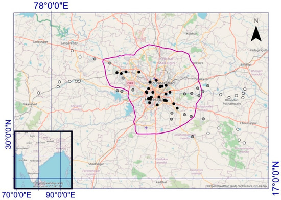
Figure 1.
Rural (white), peri-urban (grey) and urban (black) study locations in Telangana State, India. The Nehru ring road is shown in purple. Inset is a wider map showing Hyderabad within India.
2.3. Questionnaire Design
We focussed on 10 ES: drinking water, food production (rice), fuel (fuelwood and charcoal), fish, sediment regulation, hazard mitigation (flooding), sanitation [21], recreation in natural spaces, nature’s aesthetic and enjoying nature for spiritual reasons. We designed the questionnaire in English and our survey team translated it into Telegu, Urdu and Hindi (the main languages spoken in study area) in real-time as they conducted the survey. We piloted the questionnaire and translation using a sample of 30 participants comprising 50% males and 50% females from rural, peri-urban and urban areas outside of the selected sampling locations. Based on the findings of the pilot, we edited the questionnaire and translations used as required. The survey was delivered using Android-based smartphones and tablets using Open Data Kit (ODK; https://opendatakit.org/ (accessed on 20 February 2021)) to collect the survey data. We trained the enumerators with the questionnaire and the use of ODK. This training also included a trial of the survey in at least three different sites (rural, urban and peri-urban) and a feedback session with the enumerators after the trial was used to further refine the questionnaire via a small number of relatively minor edits. The University of Gloucestershire Research Ethics Committee provide ethics approval for the questionnaire survey on the 12 February 2019 (Approval code: REC.19.16.1).
Prior to the questionnaire survey, consent was obtained verbally from the respondent in each household. No sensitive data were collected, and respondents were informed that they could stop the survey at any time. All respondents were aged 18 years and above. The survey was conducted during the months of February–May 2019.
For each respondent, we collected socioeconomic data, including the respondent’s monthly income, social class, residency status, and household size. For provisioning ES (rice, fish, fuelwood/charcoal), we collected data on usage quantity, purchased quantity, received (given free of charge) quantity, price, how they obtained it, seasonal variations (excess and scarcity), where they get it (recording location on a digital map) and the ecosystem it likely originated in (again recording location). For sediment regulation and hazard, we included the cost of impact and cost of protective measures (if any), marking the location on the digital map. For sanitation, we recorded the types and location of the sanitation facility, frequency of use and marking the location of the facility on the digital map. Finally, for the cultural services (i.e., recreation, aesthetic and spirituality), we recorded the number of hours spent and money spent per week accessing these services, recording their locations on the digital map. Our full ODK survey is available here: https://github.com/InduneeWelivita/Household-survey-questionnaire-RUST-project/blob/main/household_survey_ODK.xlsx (accessed on 16 April 2021). The data are available via https://reshare.ukdataservice.ac.uk/854680/ (accessed on 16 April 2021).
As with all studies, there might be some uncertainties associated with the survey data. For example, we asked the respondents to mark the ES location on a map (i.e., where they perceived the ES to have originated, where they obtained the natural goods themselves). Thus, there is potential for such an approach to result in systematic bias. For instance, if urban inhabitants are more disconnected from nature than rural residents (e.g., as might be predicted from red loop–green loop theory) then urban people may be less likely to accurately locate the source of each ES. However, this bias is unlikely to impact the results as no question in the survey was compulsory. Therefore, if any respondent was uncertain about a question, they could (and were encouraged to) simply skip that question, rather than give an erroneous answer. As such, whilst the data collected undoubtedly contain some uncertainty (e.g., in locations or the quantities of ES used), it is unlikely to contain any systematic biases that would negate the results of our analyses.
2.4. Analysis
The data were cleaned prior to analysis to correct the typographical errors and remove any no-data values (e.g., 9999), outliers and/or other values that were not possible (see Appendix B for our full details of the data cleaning rules applied). Each ES was analysed via general linear models (GLMs) using SPSS (IBM SPSS Statistics 23). The variables used for each ES were the quantity of ES used (Equation (1)), location of where the ES was obtained (from which we calculated the distance from the ES to their household; referred to as “beneficiary travel distance”; Equation (2)), and location of where the ES originated in nature (again calculating distance to the household; termed “total ES distance”; Equation (3)). Each GLM compared one of the ES variables to the locality of the household (urban, peri-urban and rural) and how the ES was obtained (i.e., from the source themselves, from a seller, from a relative, from a friend; Equations (1)–(3)). We statistically controlled the cost per unit (if applicable), the respondent’s monthly income (as a proxy for household income), social class, residency status (owner/tenant/other), and household size as explanatory variables (Equations (1)–(3); see Appendix C for a full description of each variable). We also developed GLMs for the percentage of households at each site (Figure 1) having direct access to provisioning ES (i.e., they reported obtaining drinking water, rice, fuelwood, fish and/or sanitation themselves, as opposed to via a seller, friend or relative; Equation (4)). The statistical models only investigated the main effects as no interactions were included.
Quantity of ES used = Locality of the household + How the ES was obtained + Cost per unit (if applicable) + Monthly income + Social class + Residency status + Household size
Beneficiary travel distance = Locality of the household + How the ES was obtained + Cost per unit (if applicable) + Monthly income + Social class + Residency status + Household size
Total ES distance = Locality of the household + How the ES was obtained + Cost per unit (if applicable) + Monthly income + Social class + Residency status + Household size
Percentage of households having direct access ES = Locality of the household
3. Results
We surveyed 3010 households, yet the response rate for different ES and their variables were different as respondents were encouraged to skip questions they did not want to answer and/or they were not sure of the answer individuals could skip any question they wished, and not everyone used all ES (Table 1; Appendix D). We found that the drinking water, sanitation, recreation, aesthetic and spirituality questions were answered by a higher number of households with a lower number of responses for rice and fish, and the lowest sample size for fuelwood/charcoal, sediment regulation and hazards. The number of responses might provide an indication of the ES most familiar to the respondents (Table 1). Here, we display overall summary statistics (Table 1), before reporting the GLM results for each ES from Equations (1)–(4), respectively (see Appendix E for extended results with full coefficient tables).

Table 1.
Descriptive statistics of the ecosystem service variables.
3.1. Quantity of Ecosystem Service Used
We were not able to develop models (Equation (1)) for flood (hazard), sedimentation and erosion (sediment regulation), and charcoal as their usage was reported by too small a number of households. We were also unable to develop a statistically significant model for the time spent on spiritual activities (Adj R-sq = −0.001). All of the considered variables were statistically insignificant in this model. However, for the remaining ES we investigated, we were able to run GLMs, the findings of which are summarised below:
3.1.1. Drinking Water
Daily drinking water consumption (adjusted R-squared [Adj R-sq] = 0.557; n = 761) varied by the locality of the household (p < 0.001). Specifically, water consumption was highest in urban areas, with rural areas being 39.03 L lower (p < 0.001) and peri urban areas being 83.41 L lower (p < 0.001). Water consumption also varied by the residency status of the household (p < 0.05; being highest among tenants and “other” residency status, with owners being 58.47 L lower) and when respondents obtain it from relatives, friends or sellers (being with 41.29 L being lower when obtained by the respondent themselves; p < 0.05). Water consumption increased by 11.31 L for every person in the household (p < 0.001) and decreased by 142.81 L for every additional water source (p < 0.001) they have access to. Water quantity also decreased by 6.30 L for every INR 10 of the monthly cost of water (p < 0.05). Daily drinking water consumption varied by the type of water source (p < 0.001), being 47–81 L higher for households that water pipped into the dwelling, via a tube well or via a piped neighbour than households having tanker-truck, bottled water, protected well, unprotected well, and water kiosk sources, with households accessing public taps or with water pipped into their compound using 43–45 L less water again. The sample size of this model can be increased by dropping the “How the ES was obtained” variable from the model; however, the results are consistent (adjusted R-squared [Adj R-sq] = 0.620; n = 2669; Appendix E).
3.1.2. Sanitation
The frequency of daily toilet use (Adj R-sq = 0.173; n = 3000) increased by 20 uses for every additional three people in the household (p < 0.001). For every INR 88,731 increase in monthly income, the frequency of toilet use per day increased up by 1 (p < 0.05). The frequency of daily use also varied by the type of toilet used (p < 0.001). Frequency of use was 1.36 lower for households on site sanitation options than for households with toilet flush to a piped sewer system (p < 0.05) and 2.15 lower than households with toilet flush to open drains (p < 0.05). The frequency of daily toilet use also showed significant interaction between the locality of the household (urban, peri urban and rural) and toilet type (p < 0.001; see Appendix E for details). Frequency of daily toilet use also varied by the social class (p < 0.001), being lowest in our other category (Muslim), but 1.32 higher in the general class (p < 0.001), 0.92 higher among other backward classes (p < 0.001), 0.77 higher among scheduled tribes (p < 0.001), and 0.74 higher among scheduled castes (p < 0.001). The frequency of daily toilet use varied by the place of use (p < 0.05), being lowers in those using a neighbour’s toilet, temporary pit toilet and church toilets but 2.86 higher among public toilet users (p < 0.05), 1.72 higher among household toilet users (p < 0.05), 1.54 higher among community toilet users (p < 0.05), and 1.29 higher among people who use open defecation (p < 0.05).
3.1.3. Rice
The rice quantity purchased per week (Adj R-sq = 0.089; n = 1592) increased by 2.06 kg for every extra person in the household (p < 0.001) and by 1.18 kg for every INR 10 of the cost of rice per kg (p < 0.001). The weekly rice quantity purchased was higher when respondents bought from relatives, friends or sellers than those obtaining rice themselves, with the latter group buying 4.07 kg (p < 0.001). We also modelled the rice quantity given free of charge per week (Adj R-sq = 0.042; n = 1591). The amount of rice given (free of charge) to the respondent per week increased by 1.82 kg for every INR 10 of the cost of rice per kg (p < 0.05). We found that the given rice quantity varies by the locality of the household (p < 0.001). Specifically, the rice quantity given is lowest in urban and peri urban areas, with rural areas being 17.73 kg higher per household per week (p < 0.001).
3.1.4. Fuelwood
The fuelwood quantity used per week (Adj R-sq = 0.222; n = 46) decreased by 5.28 kg for every INR 1 of the cost of fuelwood (per kg) (p < 0.05). The fuelwood quantity use per week varied by how it was obtained (p < 0.05). This quantity was highest when respondents buy from sellers, being 66.10 kg lower when obtained by the respondents themselves (p < 0.05) and 80.16 kg lower when obtained from relatives (p < 0.05). The fuelwood quantity purchased per week (Adj R-sq = 0.677; n = 47) decreased by 6.70 kg for every INR 1 increase in cost of fuelwood per kg (p < 0.001). Fuelwood quantity purchased per week was highest when respondents buy from sellers, being 121.08 kg lower from relatives (p < 0.001) and 121.91 kg lower when obtained by the respondent themselves (p < 0.001). The fuelwood quantity received (free of charge) per week (Adj R-sq = 0.232; n = 47) decreased by 4.59 kg for every INR 1 increase in the cost of fuelwood (p < 0.05). According to the model, fuelwood quantity received was lowest in urban areas, being 9.30 kg higher in peri urban areas (p < 0.05) and 11.94 kg higher in rural areas (p < 0.05). The fuelwood quantity received per week was highest when respondents obtained the fuelwood from sellers, being 57.42 kg lower when obtained by respondents themselves (p < 0.05) and 68.25 kg lower from relatives (p < 0.05).
3.1.5. Fish
The fish quantity consumed per week (Adj R-sq = 0.275; n = 210) increased by 0.08 kg for every INR 10,000 increase in monthly income (p <0.05), by 0.01 kg for every INR 10 increase in the cost of fish and by 0.18 kg for every extra person in the household (p < 0.001). The quantity of fish they purchased per week (Adj R-sq = 0.572; n = 443) increased by 83 g for every extra person in the household (p < 0.001) and by 0.5 kg for every INR 100 increase in the price of fish per kg (p < 0.001). Weekly purchased fish quantity was highest when respondents purchased from sellers, being 0.33 kg lower when purchased from relatives (p < 0.05). The quantity of the fish they received (free of charge) per week (Adj R-sq = 0.358; n = 451) increased by 0.119 kg for every extra person in the household (p < 0.001) and by 0.4 kg for every INR 100 of the cost of fish (per kg) (p < 0.001). We also found that the fish quantity received per week was highest among ‘other’ residency status, being 0.47 kg lower among owners (p < 0.05) and 0.48 kg lower among tenants (p < 0.05) of the house.
3.1.6. Recreation in Nature
The time spent on recreational activities per week (Adj R-sq = 0.008; n = 2907) increased by 16.8 min for every INR 100,000 increase (p < 0.05) in monthly income. Weekly time spent on recreation varied by the locality of the household (p < 0.001), being highest in urban areas and peri urban areas, and 6.48 min lower in rural areas (p < 0.001). We found that the time spent on recreation in nature varied by residency status so that it is lowest among ‘other’ residency types, 14.8 min higher among tenants and 14.04 min higher among owners (p < 0.05). The money spent on recreation per week (Adj R-sq = 0.006; n = 2908) increased by INR 3.16 for every INR 10,000 increase in monthly income (p < 0.05) and decreased by INR 1.691 for every extra person in the household (p < 0.05). According to the model, weekly spending for recreation was lowest among rural and urban areas, being INR 3.641 higher among peri-urban residents (p < 0.1).
3.1.7. Enjoying Nature’s Aesthetics
The time spent enjoying nature’s aesthetics per week (Adj R-sq = 0.006; n = 2908) decreased by 43 min for every INR 100,000 increase in monthly income (p < 0.05) and by 42 min for every extra person in the household (p < 0.05) and varied by social class (p < 0.05). The money spent on aesthetics per week (Adj R-sq = 0.001; n = 2891) decreased by 3 INR for every INR 10,000 increase in monthly income (p < 0.05).
3.1.8. Visiting Nature for Spiritual Reasons
The amount of money spent on visiting nature for spiritual reasons per week (Adj R-sq = 0.004; n = 2988) increased by INR 2.86 for every INR 10,000 increase (p < 0.05) in monthly income. The money spent on spirituality per week decreased by 2.45 INR for every extra person in the household (p < 0.05). Money spent on spirituality is highest in urban areas and peri-urban areas, being INR 7.91 lower in rural areas (p < 0.05).
3.2. Total Ecosystem Service Distance
No variables were significant for models (Equation (2)) of distance between the household to the ecosystem where the fish, charcoal, and fuelwood originated (total ES distance), where they get fuelwood from, defecation location, location of flood impact, where they visit to appreciate aesthetic beauty, where they visit to enjoy recreation and place of spirituality (p > 0.05). We were unable to model the total ES distance of rice or recreational place because negative R-squared values indicated poor model performance (i.e., the response is very low or negligible [22]).
3.3. Beneficiary Travel Distance
No variables were significant for models (Equation (3)) of distance between a household to the place where they obtained charcoal and fuelwood (p > 0.05). We were unable to model the distance between a household to the place where they obtained water because negative R-squared [22]. However, for the remaining ES we investigated, the findings of which are summarised below.
3.3.1. Rice
The distance between a respondent’s household and where they obtained rice (Adj R-sq = 0.044; n = 1571) increased by 1 m for every INR 100 of the monthly income (p < 0.05). The distance was lower in peri urban and urban areas, with rural areas being 0.39 km further (p < 0.001). We also found that the distance to where they obtained rice was lower when they obtained it from the source themselves, via a friend or via a seller, while it was 2 km further when they obtained it via a relative (p < 0.001).
3.3.2. Fish
The model developed for the distance between a respondent’s household location and where they obtained fish (Adj R-sq = 0.041; n = 210) was weak yet showed significant patterns. The distance varied by social class (p < 0.05). Specifically, the distance was lowest among Scheduled Tribes, “Other Backward Class”, Scheduled castes and “other social classes”, being 3.16 km further for general class people (p < 0.05).
3.3.3. Aesthetics
The model developed for the distance between a respondent’s household and place of aesthetic beauty (Adj R-sq = 0.004; n = 1592) was weak yet showed significant patterns. The distance varied by the locality of the household (p < 0.05). Specifically, the distance was lower among urban households, being 0.25 km further among peri-urban households (p < 0.05) and 0.31 km further among rural households (p < 0.05).
3.4. Direct Access to Ecosystem Services
We developed GLMs (Equation (4)) for the percentage of households having direct access to provisioning ES (i.e., they reported obtaining drinking water, rice, fuelwood, fish and/or sanitation themselves, as opposed to via a seller, friend or relative; Table 2). The percentage of households with direct access to drinking water varied by the locality of the household (Adj R-sq = 0.179; n = 53), with the percentage higher in urban and rural areas, with peri urban areas being 17.87% lower (p < 0.001). The model developed for the percentage of households having direct access to sanitation ES (Adj R-sq = 0.769; n = 64) showed that the percentage was lower in urban areas, with peri urban areas being 55.39% higher (p < 0.001) and rural areas being 75.85% higher (p < 0.001). We were unable to develop models with statistically significant variables for rice, fuelwood and fish. Additionally, no model was developed for charcoal as their usage was reported by too small a number of households.
Table 2.
Percentage of respondents obtaining provisioning ecosystem services directly (i.e., themselves) or indirectly (e.g., via a friend, relative or seller) as per the locality of the household.
4. Discussion
Red-loop, green-loop theory predicts that rural people directly use local ES, whereas urban people tend to indirectly use services from more distant ecosystems (e.g., via a value chain) [13]. This is because many ES are locally produced in rural areas but not in urban areas and thus these services must be imported from other ecosystems by urban people [23]. Here, we achieved our aim of evaluating red-loop–green-loop theory against evidence, generally finding more similarities than differences in ES flow across the rural-urban spectrum, and so rejecting our hypotheses in most instances.
For 20% of the ES investigated, we find the direct–indirect use pattern you would expect under red-loop–green-loop theory—i.e., that rural inhabitants use ecosystem services more directly than urban residents (Table 3). However, for many ES (rice, fuelwood and fish), we find no difference in levels of direct access across rural, peri-urban and urban areas. This lack of difference between rural and urban areas might arise due to similar levels of market access in rural and urban areas (i.e., allowing indirect use of ecosystem services across the rural-urban spectrum via value chains) [15], or perhaps because our “close to city” rural is not remote enough for differences to be detected. The latter is unlikely as we were able to detect some differences for some ES. However, when we detected differences in levels of direct/indirect access, they did not necessarily reflect the patterns predicted by red-loop–green-loop theory. For example, we found that direct access to drinking water is higher in rural and urban areas, whilst indirect access highest in peri-urban areas. For rural areas, this result was expected. However, the majority of urban respondents are not getting water directly from nature and instead receive it via a socio-technical configuration of institutions and engineering infrastructure—although, interestingly, this “seller” is not perceived by our respondents. Hamann et al. [15] also found that peri-urban areas are a mixture of high and low ES direct use areas, and often not an area of intermediate level of direct use between rural and urban areas as might be predicted. The intermittent ES access in peri-urban areas is perhaps a result of poor service delivery from both city authorities and nature [24]. By contrast, we do find evidence of the expected red loop-green loop pattern for sanitation ES. Many rural areas have decentralized waste treatment (mainly having pit latrines in their households), while urban areas often rely on centralized waste treatment plants often located outside the urban areas themselves [25].
Table 3.
Summary of differences in ecosystem services (ES) flows across the rural-urban spectrum around Hyderabad. Localities where respondents reported the highest (↑), in between (↔), and lowest (↓) values are shown. Blank cells indicate no significant difference across rural, peri-urban and urban areas. ES models that could not be run (e.g., due to low sample size) are not shown.
While red-loop–green-loop theory predicts that rural residents use more local ecosystems than urban residents [13], we find no evidence of this. Our data show no significant difference in distance between the ecosystem where the ES was perceived to have been generated and where the ES was used across rural, peri-urban or urban areas (although this may differ for other ES, or if transects were extended deeper into rural areas). This is likely because, in an ever more developed and globalised world, both rural and urban residents get many of the ES they need from distant ES via value [15,26]. In five West African cities, rice is typically delivered from relatively remote areas through value chains with varying distance from 762–1602 km [27]. By contrast, the distance between the origin and consumption of rice is often smaller in rural areas where subsistence farming may be practiced; e.g., with such distances ~2 km in Sierra Leone [28] and <30 km in the Mekong Delta [28]. However, due to the public distribution system operated in India (including in our study area), people in all areas are able to access rice produced across the country [29]. Likewise, low-income households in both rural and urban areas in India rely on fuelwood from local ecosystems—i.e., from using homesteads, nearby woodlands or street trimmings from urban green spaces, respectively [30,31] By contrast, 58.2% of rural people and 80.7% of urban people in India have water facilities in their households [32]. As such, urban residents have a higher capacity to access distant water sources (via a piped water system) when compared to more rural people, who may need to retrieve water from relatively nearby on foot [33].
Whilst there is no difference in the distance between where the ES was perceived to have been generated and where the ES was used, our results show that urban people themselves travel shorter distance than rural people to access many ES (rice, and aesthetics; Table 2 and Table 3). This is likely because the urban areas have good infrastructure enabling the transport of ES to beneficiaries’ doorsteps (or relatively nearby), as well as more nearby services and shops. Previous studies show similar findings, for example, urban residents are also closer to food stores than those in rural areas [34,35]. This pattern persists even when the ES is generated more locally (i.e., within the city itself) [36]. For example, city authorities provide green spaces and parks for recreation and aesthetic beauty and religious places for spiritual services to urban people in order to increase their quality of life [37], and urban people tend to travel less to use these services than rural people [38,39]. Our results echo this, showing that urban peoples travel lower mean distances (Aesthetic ES: 187 m; Recreation ES: 141 m; and Spirituality ES: 205 m) to access these cultural services compared to rural and peri urban areas (Rural: 535 m, 465 m and 509 m, and Peri-Urban: 46 m, 974 m and 617 m, respectively).
Furthermore, we generally observe no differences in the quantity of ES used across the rural–urban spectrum (Table 3), consistent with some previous findings. For example, no differences between the amount of provisioning or regulating services used were observed between rural and urban areas in/surrounding the European cities of Berlin, Helsinki, Salzburg and Stockholm [36]. However, other studies show that provisioning services are used less in urban areas than in rural areas [40,41,42,43]. Reduced use of provisioning services in urban areas might be because higher population densities in urban areas result in high resource consumption, so often degraded ecosystems have to support higher numbers of people per unit area (and thus with less ES per person) [44,45]. Similarly, lower levels of land tenure in urban areas might result in reduced access to some ES [46,47]. For example, public green spaces in urban areas are often highly regulated and activities such as grazing, or firewood collection may be prohibited. Similarly, urbanisation often results in changed lifestyles towards those that rely more on non-ecosystem goods due to convenience and technological development (i.e., petroleum fuel/electricity for fuelwood, plastics/metal for timber etc) [37,43]. This high demand for non-natural products may lead to a lower usage of ES in urban areas. By contrast, we show that investment in cultural services in rural areas is lower than in urban areas. It is likely this pattern occurs as rural inhabitants prioritise obtaining the provisioning services required to fulfil their basic needs, with regulating and cultural services prioritised in more built-up areas where baseline living standards can be higher and many basic needs are already met [40,43,48,49,50]. Thus, use of provisioning services may be higher in rural areas, but the use of cultural services is higher in urban areas, and, where these differences in quantities of ES use exist, peri-urban areas sometimes show an intermediate step between rural and urban systems.
Within Hyderabad and the surrounding area, our results are robust, and we believe that Hyderabad can serve as a case study to represent other rapidly expanding cities across the Global South (see Section 2.1). However, it is important that these findings are validated in numerous cities across the globe before making conclusions about the global applicability of red-loop–green-loop theory. For example, it is currently not known if our findings would be replicated if this study was repeated in the Global North, and this could be an avenue for future research. Further limitations relate to the survey method used. Surveys reveal perceptions of ES flows, but beneficiaries may not be aware of the full value chain [51] nor, indeed, be aware of all the ES they are receiving [52,53]. As a result, the reported ES flows from surveys may not necessarily reflect those determined by other methods [54,55]. Furthermore, whilst we investigated differences in ES flows across the rural–urban spectrum, it should be acknowledged that ecosystems provide disservices as well as services [56], and the disservices may vary between rural and urban areas [57]. Therefore, future studies should explore any systematic biases across a variety of ES methods (e.g., surveys, focus groups, observations, modelling, etc.), as well as expanding the ES investigated to include disservices as well as additional ES.
5. Conclusions
For the majority of the ES investigated, we found no statistical differences in the quantities of ES used, the distance to the ecosystem, or the levels of direct/indirect use of ecosystems between urban, peri-urban and rural areas. This evidence represents one of the most comprehensive assessments of red-loop–green-loop theory to date but does not support the predictions of this theory and thus suggests it to be a poor conceptualisation of ES flows across the rural–urban spectrum. This result is likely because ES flows across all areas have already undergone substantial modernisation and globalisation, involving complex (and often international) value chains. As such, the impact of future urbanisation on ES flows may be limited. However, our results may indicate some broad generalisations. For example, use of provisioning services may be higher in rural areas, but use of cultural services is higher in urban areas. Similarly, urban people themselves travel shorter distances than rural people to access most ES. Furthermore, where these differences in ES flow exist, peri-urban areas sometimes show an intermediate step between rural and urban systems. Our results highlight differences in flow between ES and should be an area of development for future ES theory and research, particularly in the light of the world’s rapidly expanding urban and peri-urban populations.
Author Contributions
Conceptualization, S.W.; methodology, S.W. and I.W.; formal analysis, S.W. and I.W.; writing—original draft preparation, S.W. and I.W.; all authors were involved in data collection and in reviewing and editing the manuscript. All authors have read and agreed to the published version of the manuscript.
Funding
This research was funded by the UK’s Economic and Social Research Council and the Indian Council of Social Science Research (Grant numbers: ES/R006865/1 and ES/R009279/1).
Data Availability Statement
The data presented in this study are openly available in ReShare at https://reshare.ukdataservice.ac.uk/854680/, reference number 10.5255/UKDA-SN-854680 (accessed on 16 April 2021).
Acknowledgments
The following people are thanked for their assistance during the fieldwork: S. Anuradha, C. Vijaya Babu, M. Jyoshna, N. Kalyani, H. Kumar, M. Manikanta, M. Naresh, Pradeep, L. Pushpa, Rajesh, G. Ramesh, G. Ravinder, Santosh, B. Sharada, K. Sunitha, G. Swami, and M. Yamini. Alison Parker is thanked for comments on both the survey and the manuscript. Finally, we thank the anonymous reviewers.
Conflicts of Interest
The authors declare no conflict of interest. The funders had no role in the design of the study; in the collection, analyses, or interpretation of data; in the writing of the manuscript, or in the decision to publish the results.
Appendix A. Transect Population Density Range

Figure A1.
The local population density (from worldpop.com) of our survey respondents categorised by using our rural, peri-urban and urban divisions.
Figure A1.
The local population density (from worldpop.com) of our survey respondents categorised by using our rural, peri-urban and urban divisions.

Appendix B. Data Cleaning Rules
Table A1.
Cleaning rules for numerical data.
Table A1.
Cleaning rules for numerical data.
| Data Range | Cleaning Rule |
|---|---|
| Water quantity—daily | |
| 0–3000 and 9999 L | For the data on daily water usage data (for drinking, cooking and bathing), values were identified as erroneous is they exceeded 698.9 L, which is the maximum water quantity for drinking, cooking and bathing, according to the study done in Rajasthan, India (Choudhary et al., 2012). If they did exceed 698.9 L, they were removed. This correction was required for 26 out of 4458 entries (0.58%). Further, 9999 values were deleted as this was used to mark “do not know” answers in previous columns. This correction was required for 4 out of 4458 households (0.08%). |
| Willingness to pay for water (per month) | |
| INR 0–800 and 9999 | According to the local collaborating partners, it is possible to have INR 990 per month as a maximum. Therefore, all data were kept except 9999 values. This correction was required for 8 data points out of 3011 entries (0.26%). |
| Monthly water bill | |
| INR 0–6223 and 9999 | According to the local collaborating partners, monthly water bills cannot be less than INR 10 or more than INR 990. We removed the values less than 10 but we kept zero as in some areas the water bill was zero. Again, we removed the values more than INR 990. This correction was required for 76 values out of 4458 entries. Additionally, we removed 999,999,999,999 mistakenly added for “don’t know” responses. This correction was required for 384 out of 4458 entries (8.61%). |
| Waste quantity—daily | |
| 0–50 kg | For the data on daily household waste quantity, values were identified as erroneous if they exceeded a maximum value of 4.14 kg according to the study done in Dehradun city, India (Suthar and Singh, 2015). These were removed and this correction was required for 28 out of 2896 households (1.00%). |
| Rice quantity purchased—last week | |
| 0–600 kg | According to the local collaborating partners, it is possible to store large quantities of rice purchased for a long period of time. All of the data for quantity of rice purchased (last week) by a household were kept. |
| Rice cost—per kg | |
| INR 0–800 | For the data on cost of rice (per kilo gram), values were identified and removed as erroneous if they exceeded INR 100 according to the Indiamart.com website. This correction was required for 9 out of 1715 households (0.52%). Additionally, we removed rice price values given by the respondents who said that no rice had been purchased that week. This correction was required for 50 out of 1715 households (2.9%). |
| Rice received—last week | |
| 0–2000 kg | According to the local collaborating partners, it is possible to store large quantities of rice received from relatives or friends for a long time period. For the data on quantity of rice received (last week) by a household, all the data were kept. |
| Recreation expense—last week | |
| INR 0–5000 and 9999 | For the data on recreation expense (last week), values were identified as erroneous if they exceeded 11.65% of the monthly income according to Upadhyay and Pathania (2013). We assumed that their non-food expenses all go to recreation, and weekly given expenses are the only non-food expenses per month. From this we calculated the share of non-food expenses. If they did exceed that value, they were removed. This correction was required for 4 out of 2853 households (0.14%). |
| Recreation hours—last week | |
| 0–888 h & 9999 | For the data on recreation hours, we identified values as erroneous if they exceeded 84 h because it is unrealistic that people spend more than 12 h a day 7 days a week on recreational activities. If they did exceed 84, we deleted the value. This correction was required for 3 data points (0.10%). |
| Aesthetic expense—last week | |
| INR 0–10,000 and 9999 | For the data on aesthetic expense (last week), values were identified as erroneous if they exceeded 11.65% of the monthly income according to Upadhyay and Pathania (2013). We assumed that their non-food expenses all go to aesthetic, and weekly given expense is the only non-food expenses per month. Then, we calculated the share of non-food expenses. If they did exceed that value, they were removed. This correction was required for 6 out of 2850 households (0.21%). |
| Aesthetic hours—last week | |
| 0–2400 h & 9999 | For the data on aesthetic hours, we identified values as erroneous if they exceeded 84 h because it is unrealistic that people spend more than 12 h a day 7 days a week on aesthetic activities. If they did exceed 84, we deleted the value. This correction was required for 4 data points (0.13%). |
| Spiritual expense—last week | |
| INR 0–5000 | For the data on spiritual expense (last week), values were identified as erroneous if they exceeded 11.65% of the monthly income according to [58]. We assumed that their non-food expenses all go to spiritual expenses, and weekly given expense is the only non-food expenses per month. Then, we calculated the share of non-food expenses. If they did exceed that value, they were removed. This correction was required for 6 out of 2935 households (0.043%). |
| Spiritual hours—last week | |
| 0–10,000 h | For the data on spiritual hours, we identified values as erroneous if they exceeded 84 h because it is unrealistic that people spend more than 12 h a day 7 days a week in a temple. If they did exceed 84, we deleted the value. This correction was required for 2 data points (0.06%). |
| Fish quantity consumed—last week | |
| 0–200 kg | For the data on weekly fish consumption, values were identified as erroneous if they exceeded 5 kg according to the local knowledge from our collaborating partners. If they did exceed 5 kg, they were removed. This correction was required for 5 out of 340 households (1.47%) |
| Fish quantity purchased—last week | |
| 0–1500 kg | For the data on weekly fish quantity purchased, values were identified as erroneous if they exceeded 5 kg according to the local knowledge from our collaborating partners. If they did exceed 5 kg, they were removed. This correction was required for 15 out of 572 households (2.6%). |
| Fish cost—per kg | |
| INR 0–800 and 9999 | For the data on cost of fish (per kg), values were identified as erroneous if they were 9999 because they were given “Don’t know” responses in other data columns. This correction was required for 8 out of 572 households (1.39%). Additionally, the fish cost values were removed when they had zero in the adjacent column to where the quantity of fish they purchased was asked. This correction was required for 8 out of 572 households (1.39%). The highest price for tiger prawns, which was most expensive type, does not exceed INR 1000 (Indiamart.com). There were no values more than 1000 in our data set. |
| Fish quantity received—last week | |
| 0–500 kg | For the data on weekly fish quantity received, values were identified as erroneous if they exceeded 5 kg according to the local knowledge from our collaborating partners. If they did exceed 5 kg, they were removed. This correction was required for 5 out of 572 households (0.87%). |
Appendix C. Description of the Variables
Table A2.
Description of the variables.
Table A2.
Description of the variables.
| Variable Name | Variable Type | Variable Description |
|---|---|---|
| Water quantity | Dependent | Water quantity used by a household per day (L) |
| Sanitation—toilet usage | Dependent | Number of times using the toilet by the household per day |
| Rice—purchased quantity | Dependent | Quantity of rice purchased by the household per week (kg) |
| Rice—received quantity | Dependent | Quantity of rice given to the household free of charge per week (kg) |
| Fuelwood quantity consumed | Dependent | Quantity of fuelwood used by the household per week (kg) |
| Fuelwood quantity purchased | Dependent | Quantity of fuelwood purchased by the household per week (kg) |
| Fuelwood quantity received | Dependent | Quantity of fuelwood given to the household free of charge per week (kg) |
| Fish—quantity consumed | Dependent | Quantity of fish consumed by the household per week (kg) |
| Fish—purchased quantity | Dependent | Quantity of fish purchased by the household per week (kg) |
| Fish—received quantity | Dependent | Quantity of fish given to the household free of charge per week (kg) |
| Recreational hours | Dependent | Number of hours spent in recreational places per week |
| Recreational expenses | Dependent | Amount of money spent on recreation per week (INR) |
| Aesthetic hours | Dependent | Number of hours spent for aesthetic per week |
| Aesthetic expenses | Dependent | Amount of money spent on aesthetic per week (INR) |
| Spirituality hours | Dependent | Number of hours spent on spirituality per week |
| Spirituality expenses | Dependent | Amount of money spent on spirituality per week (INR) |
| Rice—ES distance | Dependent | Distance between household and origin of rice |
| Fuelwood—ES distance | Dependent | Distance between household and origin of fuelwood |
| Fish—ES distance | Dependent | Distance between household and origin of fish |
| Water—travel distance | Dependent | Distance between household and where they get water |
| Sanitation—toilet travel distance | Dependent | Distance between household and location of toilet |
| Rice—travel distance | Dependent | Distance between household and where they get rice |
| Fuelwood—travel distance | Dependent | Distance between household and where they get fuelwood |
| Fish—travel distance | Dependent | Distance between household and where they get fish |
| Recreation—travel distance | Dependent | Distance between household and where they enjoy recreation |
| Aesthetic—travel distance | Dependent | Distance between household and where they enjoy aesthetic beauty |
| Spirituality—travel distance | Dependent | Distance between household and where they go for spirituality |
| Area—peri urban | Independent | Household is located in a peri-urban area |
| Area—rural | Independent | Household is located in a rural area |
| Area—urban | Independent | Household is located in an urban area |
| Social class—General | Independent | Social class of the respondent household |
| Social class—Other Backward Class (OBT) | Independent | Social class of the respondent household |
| Social class—Scheduled caste | Independent | Social class of the respondent household |
| Social class—Scheduled tribes | Independent | Social class of the respondent household |
| Residency status—owner | Independent | Residency status of the household |
| Residency status—tenant | Independent | Residency status of the household |
| Residency status—other | Independent | Residency status of the household |
| Household size | Independent | Number of members in the household |
| Monthly income (INR) | Independent | Monthly income of the household (INR) |
| Water use—drinking | Independent | Using the particular water source for drinking (Yes/No) |
| Water use—cooking | Independent | Using the particular water source for cooking (Yes/No) |
| Water use—bathing | Independent | Using the particular water source for bathing (Yes/No) |
| Water source—11 | Independent | Water piped into dwelling |
| Water source—12 | Independent | Water piped into compound, yard or plot |
| Water source—13 | Independent | Water piped to neighbour |
| Water source—14 | Independent | Public tap (standpipe) |
| Water source—21 | Independent | Tube Well/Borehole |
| Water source—61 | Independent | Tanker-truck |
| Water source—72 | Independent | Water kiosk |
| Water source—91 | Independent | Bottled water |
| Water source—99 | Independent | Other (specify) |
| Water collected by—1 | Independent | Water collected for the household by themselves |
| Water collected by—2 | Independent | Water collected for the household by friends |
| Water collected by—3 | Independent | Water collected for the household by relatives |
| Water collected by—4 | Independent | Water collected for the household by sellers |
| Number of different water sources | Independent | Number of different water sources they are using? |
| Household level water purification—done | Independent | Purifying the water at household |
| Household water purification expense per month (INR) | Independent | Cost of purifying the water at household per month (INR) |
| Cost of water (month) (INR) | Independent | Cost of water per month (INR) |
| Place of the toilet—1 | Independent | Household toilet |
| Place of the toilet—2 | Independent | Community toilet |
| Place of the toilet—3 | Independent | Public toilet |
| Place of the toilet—4 | Independent | Open defecation |
| Place of the toilet-other | Independent | Other please specify (workplace toilet, etc.) |
| Type of the toilet—11 | Independent | Toilet flush to piped sewer system |
| Type of the toilet—12 | Independent | Toilet flush to septic tank |
| Type of the toilet—13 | Independent | Toilet flush to pit latrine |
| Type of the toilet—14 | Independent | Toilet flush to open drain |
| Type of the toilet—22 | Independent | Pit latrine with slab |
| Type of the toilet—23 | Independent | Pit latrine without slab/Open pit |
| Type of the toilet—31 | Independent | Composting toilet |
| Type of the toilet—32 | Independent | Twin pit toilet with slab |
| Type of the toilet—41 | Independent | Bucket toilet |
| Type of the toilet—other | Independent | Open defecation |
| Rice source—themselves | Independent | Rice collected for the household by themselves |
| Rice source—via friend | Independent | Rice collected for the household by friends |
| Rice source—via relative | Independent | Rice collected for the household by relatives |
| Rice source—via seller | Independent | Rice collected for the household by sellers |
| Rice purchased cost (INR) | Independent | Cost of rice per week (INR) |
| Fuelwood source—themselves | Independent | Fuelwood collected for the household by themselves |
| Fuelwood source—via relative | Independent | Fuelwood collected for the household by relatives |
| Fuelwood source—via seller | Independent | Fuelwood collected for the household by sellers |
| Fuelwood purchased cost (INR) | Independent | Cost of fuelwood per week (INR) |
| Fish source—via relative | Independent | Fish collected for the household by relatives |
| Fish source—via seller | Independent | Fish collected for the household by sellers |
| Fish purchased cost (INR) | Independent | Cost of fish per week (INR) |
Table A3.
Description of the category codes.
Table A3.
Description of the category codes.
| Water Source | Name of the Water Source |
| Water source—11 | Piped into dwelling |
| Water source—12 | Piped into compound, yard or plot |
| Water source—13 | Piped to neighbour |
| Water source—14 | Public tap/standpipe |
| Water source—21 | Tube Well, Borehole |
| Water source—31 | Protected well |
| Water source—32 | Unprotected well |
| Water source—42 | Unprotected spring |
| Water source—61 | Tanker-truck |
| Water source—72 | Water kiosk |
| Water source—91 | Bottled water |
| Water source—92 | Sachet water |
| Water source—99 | Other (specify) |
| Place of Toilet | Name of the Toilet Place |
| Place of the toilet—1 | Household toilet |
| Place of the toilet—2 | Community toilet |
| Place of the toilet—3 | Public toilet |
| Place of the toilet—4 | Open defecation |
| Place of the toilet—99 | Other (specify) |
| Type of the Toilet | Name of the Toilet Type |
| Type of the toilet—11 | Flush to piped sewer system |
| Type of the toilet—12 | Flush to septic tank |
| Type of the toilet—13 | Flush to pit latrine |
| Type of the toilet—14 | Flush to open drain |
| Type of the toilet—22 | Pit latrine with slab |
| Type of the toilet—23 | Pit latrine without slab/Open pit |
| Type of the toilet—31 | Composting toilet |
| Type of the toilet—32 | Twin pit with slab |
| Type of the toilet—41 | Bucket |
| Type of the toilet—other | Other (specify) |
Appendix D. Descriptive Statistics of the Respondents
Table A4.
Descriptive statistics of the respondents.
Table A4.
Descriptive statistics of the respondents.
| Variable | Groups | Count | Percentage |
|---|---|---|---|
| Household size | ≤2 | 1271 | 42.20 |
| 3–4 | 1490 | 49.50 | |
| 5–6 | 209 | 6.90 | |
| 7–8 | 27 | 0.90 | |
| 9+ | 11 | 0.40 | |
| Monthly income of the household (INR) | ≤20,000.00 | 2376 | 78.94 |
| 20,001.00–40,000.00 | 542 | 18.01 | |
| 40,001.00–60,000.00 | 76 | 2.53 | |
| 60,001.00–80,000.00 | 11 | 0.37 | |
| 80,001.00–100,000.00 | 1 | 0.03 | |
| 100,001.00–120,000.00 | 2 | 0.06 | |
| 120,001.00+ | 2 | 0.06 | |
| Social class | General | 305 | 10.10 |
| OBC | 1679 | 55.80 | |
| ST | 788 | 26.20 | |
| ST | 193 | 6.40 | |
| Other | 42 | 1.40 | |
| Residency status | Owner | 2193 | 72.90 |
| Tenant | 739 | 24.60 | |
| 99 | 76 | 2.50 |
Appendix E. Extended Results
Table A5.
Ecosystem service quantification (for variable descriptions see Appendix C).
Table A5.
Ecosystem service quantification (for variable descriptions see Appendix C).
| Ecosystem Service Variable | Parameter | Coefficient | p-Value |
|---|---|---|---|
| Daily drinking water consumption | Water source—11 | 81.44 | 5.56 × 10⁻¹¹ |
| Water source—12 | −43.52 | 3.94 × 10⁻³ | |
| Water source—13 | 47.85 | 4.10 × 10⁻² | |
| Water source—14 | −45.01 | 3.09 × 10⁻³ | |
| Water source—21 | 69.65 | 3.04 × 10⁻³ | |
| Water source—31 | 34.18 | 5.11 × 10⁻¹ | |
| Water source—32 | 35.86 | 6.81 × 10⁻¹ | |
| Water source—42 | 118.94 | 1.73 × 10⁻¹ | |
| Water source—61 | −32.40 | 2.46 × 10⁻¹ | |
| Water source—72 | 0.25 | 9.84 × 10⁻¹ | |
| Water source—91 | −0.83 | 9.40 × 10⁻¹ | |
| Water source—92 | 171.50 | 5.41 × 10⁻¹ | |
| Water source—99 | 0 | ||
| Area—peri urban | −39.03 | 9.10 × 10⁻⁵ | |
| Area—rural | −83.41 | 2.23 × 10⁻¹³ | |
| Area—urban | 0 | ||
| Social class—General | 33.87 | 3.47 × 10⁻¹ | |
| Social class—Other Backward Class (OBT) | 54.81 | 1.09 × 10⁻¹ | |
| Social class—Scheduled caste | 44.71 | 1.94 × 10⁻¹ | |
| Social class—Scheduled tribes | 60.48 | 0.93 × 10⁻¹ | |
| Social class—other | 0 | ||
| Residency status—owner | −58.47 | 7.64 × 10⁻³ | |
| Residency status—tenant | −7.79 × 10⁻¹ | 9.37 × 10⁻¹ | |
| Residency status—other | 0 | ||
| Water collected by—themselves | −41.297 | 4.40 × 10⁻³¹ | |
| Water collected by—friend | −24.067 | 5.98 × 10⁻¹ | |
| Water collected by—relative | −16.063 | 4.95 × 10⁻¹ | |
| Water collected by—seller | 0 | ||
| Number of different water sources | −142.81 | 7.188 × 10−47 | |
| Cost of water (month) (INR) | −0.06 | 2.85 × 10⁻² | |
| Household size | 11.31 | 1.00 × 10⁻⁶ | |
| Monthly income (INR) | −5.90 × 10⁻⁵ | 8.71 × 10⁻¹ | |
| Daily drinking water consumption excluding the “How the ES was obtained” variable | Water source—11 | 98.018 | 1.19 × 10⁻³³ |
| Water source—12 | 59.201 | 7.08 × 10⁻¹⁰ | |
| Water source—13 | 79.896 | 1.05 × 10⁻⁸ | |
| Water source—14 | 19.278 | 4.76 × 10⁻² | |
| Water source—21 | 70.141 | 2.59 × 10⁻⁷ | |
| Water source—31 | 59.575 | 1.69 × 10⁻¹ | |
| Water source—32 | 44.013 | 5.99 × 10⁻¹ | |
| Water source—42 | 136.852 | 1.03 × 10⁻¹ | |
| Water source—61 | 64.225 | 3.00 × 10⁻⁶ | |
| Water source—72 | −5.035 | 6.10 × 10⁻¹ | |
| Water source—91 | 8.027 | 2.23 × 10⁻¹ | |
| Water source—92 | 104.013 | 0.82 × 10⁻¹ | |
| Water source—99 | 0 | ||
| Area-peri urban | −35.577 | 1.25 × 10⁻¹² | |
| Area—rural | −57.189 | 2.15 × 10⁻²⁶ | |
| Area—urban | 0 | ||
| Social class—General | 39.342 | 1.21 × 10⁻² | |
| Social class—Other Backward Class (OBT) | 15.359 | 3.04 × 10⁻¹ | |
| Social class—Scheduled caste | 8.877 | 5.58 × 10⁻¹ | |
| Social class—Scheduled tribes | 19.192 | 2.38 × 10⁻¹ | |
| Social class—other | 0 | ||
| Residency status—owner | −53.548 | 1.80 × 10⁻⁵ | |
| Residency status—tenant | 4.162 | 3.16 × 10⁻¹ | |
| Residency status—other | 0 | ||
| Number of different water sources | −97.915 | 0 | |
| Cost of water (month) (INR) | −042 | 3.44 × 10⁻³ | |
| Household size | 18.970 | 1.97 × 10−52 | |
| Monthly income (INR) | 3.75 × 10⁻⁴ | 1.52 × 10⁻² | |
| Sanitation-toilet usage per day | Area—peri urban | 0.62 | 0.08 |
| Area—rural | 0.33 | 0.39 | |
| Area—urban | 0 | ||
| Social class—General | 1.32 | 1.90 × 10⁻⁵ | |
| Social class—Other Backward Class (OBT) | 0.92 | 1.72 × 10⁻⁵ | |
| Social class—Scheduled caste | 0.74 | 0.01 | |
| Social class—Scheduled tribes | 0.77 | 0.01 | |
| Social class—other responses | 0 | 0 | |
| Residency status—owner | 0.04 | 0.87 | |
| Residency status—tenant | −0.16 | 0.56 | |
| Residency status—other | 0 | ||
| Household size | 0.15 | 9.49 × 10⁻¹⁰ | |
| Monthly income (INR) | 1.12 × 10⁻⁵ | 6.65 × 10⁻⁴ | |
| Place of the toilet—1 | 1.72 | 7.05 × 10⁻⁴ | |
| Place of the toilet—2 | 1.54 | 0.01 | |
| Place of the toilet—3 | 2.86 | 1.25 × 10⁻³ | |
| Place of the toilet—4 | 1.29 | 0.05 | |
| Place of the toilet—99 | 0 | ||
| Type of the toilet—11 | 1.36 | 0.01 | |
| Type of the toilet—12 | 0.01 | 0.98 | |
| Type of the toilet—13 | 1.40 | 0.25 | |
| Type of the toilet—14 | 2.15 | 7.51 × 10⁻⁴ | |
| Type of the toilet—22 | −0.10 | 0.85 | |
| Type of the toilet—23 | −0.43 | 0.82 | |
| Type of the toilet—31 | 0.36 | 0.85 | |
| Type of the toilet—32 | 0.09 | 0.91 | |
| Type of the toilet—41 | 0.53 | 0.60 | |
| Type of the toilet—99 | 0 | ||
| Type of the toilet × Area—PU × 11 | −1.03 | 0.01 | |
| Type of the toilet × Area—PU × 12 | 0.59 | 0.21 | |
| Type of the toilet × Area—PU × 13 | −0.18 | 0.87 | |
| Type of the toilet × Area—PU × 14 | −1.66 | 4.58 × 10⁻³ | |
| Type of the toilet × Area—PU × 22 | 2.38 | 1.04 × 10⁻⁸ | |
| Type of the toilet × Area—PU × 23 | 0.75 | 0.71 | |
| Type of the toilet × Area—PU × 31 | −1.56 | 0.56 | |
| Type of the toilet × Area—PU × 32 | −0.13 | 0.92 | |
| Type of the toilet × Area—PU × 41 | −0.32 | 0.78 | |
| Type of the toilet × Area—PU × 95 | 0 | ||
| Type of the toilet × Area—R × 11 | −0.81 | 0.22 | |
| Type of the toilet × Area—R × 12 | 0.53 | 0.28 | |
| Type of the toilet × Area—R × 13 | −1.96 | 0.11 | |
| Type of the toilet × Area—R × 14 | −2.11 | 0.01 | |
| Type of the toilet × Area—R × 22 | 2.28 | 4.58 × 10⁻³ | |
| Type of the toilet × Area—R × 23 | −1.29 | 0.62 | |
| Type of the toilet × Area—R × 32 | 0 | ||
| Type of the toilet × Area—R × 41 | 0.24 | 0.83 | |
| Type of the toilet × Area—R × 95 | 0 | ||
| Type of the toilet × Area—U × 11 | 0 | ||
| Type of the toilet × Area—U × 12 | 0 | ||
| Type of the toilet × Area—U × 13 | 0 | ||
| Type of the toilet × Area—U × 14 | 0 | ||
| Type of the toilet × Area—U × 22 | 0 | ||
| Type of the toilet × Area—U × 23 | 0 | ||
| Type of the toilet × Area—U × 31 | 0 | ||
| Type of the toilet × Area—U × 41 | 0 | ||
| Type of the toilet × Area—U × 95 | 0 | ||
| Rice-purchased quantity | Area—peri urban | −0.64 | 0.42 |
| Area—rural | −1.46 | 0.07 | |
| Area—urban | 0 | ||
| Social class—General | 1.98 | 0.51 | |
| Social class—Other Backward Class (OBT) | −0.81 | 0.77 | |
| Social class—Scheduled caste | −0.39 | 0.88 | |
| Social class—Scheduled tribes | −0.93 | 0.75 | |
| Social class—other | 0 | ||
| Residency status–owner | −1.07 | 0.64 | |
| Residency status–tenant | −1.55 | 0.514 | |
| Residency status–other | 0 | ||
| Household size | 2.06 | 2.09 × 10⁻¹⁸ | |
| Monthly income (INR) | −2.65 × 10⁻⁵ | 0.39 | |
| Rice source–themselves | −4.07 | 8.0 × 10⁻⁶ | |
| Rice source–via friend | 0.25 | 0.94 | |
| Rice source–via relative | 1.43 | 0.54 | |
| Rice source–via seller | 0 | ||
| Rice purchased cost (INR) | 0.11 | 3.31 × 10⁻⁹ | |
| Rice-received quantity | Area–peri urban | −3.02 | 0.27 |
| Area–rural | 17.73 | 1.39 × 10⁻⁹ | |
| Area–urban | 0 | ||
| Social class–General | −7.59 | 0.46 | |
| Social class–Other Backward Class (OBT) | −2.92 | 0.76 | |
| Social class–Scheduled caste | −1.64 | 0.86 | |
| Social class–Scheduled tribes | −10.91 | 0.29 | |
| Social class–other | 0 | ||
| Residency status–owner | 0.07 | 0.99 | |
| Residency status–tenant | −0.34 | 0.96 | |
| Residency status–other | 0 | ||
| Household size | −0.19 | 0.81 | |
| Monthly income (INR) | −1.30 × 10⁻⁵ | 0.90 | |
| Rice source–themselves | 1.79 | 0.57 | |
| Rice source–via friend | 18.96 | 0.16 | |
| Rice source–via relative | 4.53 | 0.59 | |
| Rice source–via seller | 0 | ||
| Rice purchased cost (INR) | 0.18 | 8.76 × 10⁻³ | |
| Fuelwood quantity consumed | Area–peri urban | 1.476 | 0.68 |
| Area–rural | −1.66 | 0.73 | |
| Area–urban | 0 | ||
| Social class–General | −17.13 | 0.26 | |
| Social class–Other Backward Class (OBT) | −3.81 | 0.77 | |
| Social class–Scheduled caste | −1.16 | 0.92 | |
| Social class–Scheduled tribes | −1.80 | 0.89 | |
| Social class–other | 0 | ||
| Residency status–owner | 3.86 | 0.51 | |
| Residency status–tenant | −1.14 | 0.82 | |
| Residency status–other | 0 | ||
| Household size | −0.90 | 0.43 | |
| Monthly income (INR) | 1.51 × 10⁻⁴ | 0.37 | |
| Fuelwood source–themselves | −66.10 | 1.05 × 10⁻³ | |
| Fuelwood source–via relative | −80.16 | 5.69 × 10⁻⁴ | |
| Fuelwood source–via seller | 0 | ||
| Fuelwood purchased cost (INR) | −5.28 | 2.38 × 10⁻³ | |
| Fuelwood quantity purchased | Area—peri urban | −0.82 | 0.85 |
| Area—rural | 1.92 | 0.74 | |
| Area—urban | 0 | ||
| Social class—General | −35.73 | 0.05 | |
| Social class—Other Backward Class (OBT) | −32.29 | 0.04 | |
| Social class—Scheduled caste | −37.31 | 0.01 | |
| Social class—Scheduled tribes | −33.64 | 0.03 | |
| Social class—other | 0 | ||
| Residency status—owner | 8.07 | 0.25 | |
| Residency status—tenant | 8.01 | 0.20 | |
| Residency status—other | 0 | ||
| Household size | 0.33 | 0.81 | |
| Monthly income (INR) | −1.73 × 10⁻⁴ | 0.39 | |
| Fuelwood source—themselves | −121.91 | 4.00 × 10⁻⁶ | |
| Fuelwood source—via relative | −121.08 | 3.01 × 10⁻⁵ | |
| Fuelwood source—via seller | 0 | ||
| Fuelwood purchased cost (INR) | −6.70 | 1.35 × 10⁻³ | |
| Fuelwood quantity received | Area—peri urban | 9.30 | 0.01 |
| Area—rural | 11.94 | 0.01 | |
| Area—urban | 0 | ||
| Social class—General | −7.24 | 0.62 | |
| Social class—Other Backward Class (OBT) | −8.16 | 0.51 | |
| Social class—Scheduled caste | −2.52 | 0.83 | |
| Social class—Scheduled tribes | −2.42 | 0.84 | |
| Social class—other | 0 | ||
| Residency status—owner | −7.76 | 0.17 | |
| Residency status—tenant | −6.18 | 0.21 | |
| Residency status—other | 0 | ||
| Household size | −0.97 | 0.38 | |
| Monthly income (INR) | 0 | ||
| Fuelwood source—themselves | −57.42 | 2.51 × 10⁻³ | |
| Fuelwood source—via relative | −68.25 | 1.76 × 10⁻³ | |
| Fuelwood source—via seller | 0 | ||
| Fuelwood purchased cost (INR) | −4.598 | 5.07 × 10⁻³ | |
| Fish—quantity consumed | Area—peri urban | 0.16 | 0.10 |
| Area—rural | −0.02 | 0.83 | |
| Area—urban | 0 | ||
| Social class—General | −0.09 | 0.68 | |
| Social class—Other Backward Class (OBT) | −0.02 | 0.90 | |
| Social class—Scheduled caste | 0.01 | 0.92 | |
| Social class—Scheduled tribes | −0.15 | 0.50 | |
| Social class—other | 0 | ||
| Residency status—owner | 0.01 | 0.94 | |
| Residency status—tenant | 0.05 | 0.84 | |
| Residency status—other | 0 | ||
| Household size | 0.18 | 8.41 × 10⁻¹¹ | |
| Monthly income (INR) | 8.17 × 10⁻⁶ | 0.01 | |
| Fish source—via relative | 0.01 | 0.94 | |
| Fish source—via seller | 0 | ||
| Fish purchased cost (INR) | 9.94 × 10⁻⁴ | 0.03 | |
| Fish—purchased quantity | Area—peri urban | 0.05 | 0.27 |
| Area—rural | 0.10 | 0.06 | |
| Area—urban | 0 | ||
| Social class—General | 0.09 | 0.49 | |
| Social class—Other Backward Class (OBT) | 0.14 | 0.28 | |
| Social class—Scheduled caste | 0.05 | 0.70 | |
| Social class—Scheduled tribes | −0.04 | 0.78 | |
| Social class—other | 0 | ||
| Residency status—owner | −0.25 | 0.05 | |
| Residency status—tenant | −0.30 | 0.02 | |
| Residency status—other | 0 | ||
| Household size | 0.08 | 1.63 × 10⁻⁷ | |
| Monthly income (INR) | −4.38 × 10⁻⁷ | 0.82 | |
| Fish source—via relative | −0.33 | 0.01 | |
| Fish source—via seller | 0 | ||
| Fish purchased cost (INR) | 5.73 × 10⁻³ | 1.23 × 10−75 | |
| Fish—received quantity | Area—peri urban | 0.09 | 0.15 |
| Area—rural | 0.15 | 0.05 | |
| Area—urban | 0 | ||
| Social class—General | 0.01 | 0.95 | |
| Social class—Other Backward Class (OBT) | −0.01 | 0.94 | |
| Social class—Scheduled caste | −0.06 | 0.74 | |
| Social class—Scheduled tribes | −0.21 | 0.32 | |
| Social class—other | 0 | ||
| Residency status—owner | −0.47 | 5.73 × 10⁻³ | |
| Residency status—tenant | −0.48 | 5.33 × 10⁻³ | |
| Residency status—other | 0 | ||
| Household size | 0.11 | 3.79 × 10⁻⁸ | |
| Monthly income (INR) | 1.91 × 10⁻⁶ | 0.46 | |
| Fish source—via relative | 0.04 | 0.79 | |
| Fish source—via seller | 0 | ||
| Fish purchased cost (INR) | 4.27 × 10⁻³ | 4.67 × 10⁻³⁵ | |
| Recreational hours | Area—peri urban | 0.05 | 0.13 |
| Area—rural | −0.10 | 5.90 × 10⁻³ | |
| Area—urban | 0 | ||
| Social class—General | 9.23 × 10⁻³ | 0.94 | |
| Social class—Other Backward Class (OBT) | 0.08 | 0.49 | |
| Social class—Scheduled caste | 0.02 | 0.83 | |
| Social class—Scheduled tribes | 0.08 | 0.57 | |
| Social class—other | 0 | ||
| Residency status—owner | 0.23 | 0.01 | |
| Residency status—tenant | 0.24 | 0.01 | |
| Residency status—other | 0 | ||
| Household size | −3.48 × 10⁻³ | 0.76 | |
| Monthly income (INR) | −2.87 × 10⁻⁶ | 0.05 | |
| Recreational expenses | Area—peri urban | 3.64 | 0.09 |
| Area—rural | −3.03 | 0.17 | |
| Area—urban | 0 | ||
| Social class—General | 1.80 | 0.81 | |
| Social class—Other Backward Class (OBT) | 3.17 | 0.66 | |
| Social class—Scheduled caste | 2.72 | 0.71 | |
| Social class—Scheduled tribes | 2.40 | 0.76 | |
| Social class—other | 0 | ||
| Residency status—owner | 9.23 | 0.10 | |
| Residency status—tenant | 7.52 | 0.19 | |
| Residency status—other | 0 | ||
| Household size | −1.69 | 9.45 × 10⁻³ | |
| Monthly income (INR) | 3.16 × 10⁻⁴ | 1.58 × 10⁻⁴ | |
| Aesthetic hours | Area—peri urban | 0.1 | 0.2 |
| Area—rural | −0.01 | 0.92 | |
| Area—urban | 0 | ||
| Social class—General | 1.32 × 10⁻⁴ | 1.00 | |
| Social class—Other Backward Class (OBT) | 0.19 | 0.59 | |
| Social class—Scheduled caste | −0.07 | 0.84 | |
| Social class—Scheduled tribes | −0.26 | 0.51 | |
| Social class—other | 0 | ||
| Residency status—owner | 0.45 | 0.11 | |
| Residency status—tenant | 0.52 | 0.07 | |
| Residency status—other | 0 | ||
| Household size | 0.07 | 0.03 | |
| Monthly income (INR) | −8.51 × 10⁻⁶ | 0.04 | |
| Aesthetic expenses | Area—peri urban | 0.70 | 0.84 |
| Area—rural | 1.63 | 0.65 | |
| Area—urban | 0 | ||
| Social class—General | 17.23 | 0.17 | |
| Social class—Other Backward Class (OBT) | 13.79 | 0.25 | |
| Social class—Scheduled caste | 11.61 | 0.34 | |
| Social class—Scheduled tribes | 6.87 | 0.60 | |
| Social class—other | 0 | ||
| Residency status—owner | 15.76 | 0.08 | |
| Residency status—tenant | 14.98 | 0.11 | |
| Residency status—other | 0 | ||
| Household size | −0.54 | 0.61 | |
| Monthly income (INR) | 2.96 × 10⁻⁴ | 0.03 | |
| Spirituality hours | Area—peri urban | −0.06 | 0.63 |
| Area—rural | 0.12 | 0.36 | |
| Area—urban | 0 | ||
| Social class—General | 0.01 | 0.98 | |
| Social class—Other Backward Class (OBT) | 0.22 | 0.62 | |
| Social class—Scheduled caste | 0.20 | 0.66 | |
| Social class—Scheduled tribes | 0.37 | 0.45 | |
| Social class—other | 0 | ||
| Residency status—owner | 0.18 | 0.60 | |
| Residency status—tenant | 0.10 | 0.76 | |
| Residency status—other | 0 | ||
| Household size | 0.05 | 0.16 | |
| Monthly income (INR) | −6.90 × 10⁻⁶ | 0.17 | |
| Spirituality expenses | Area—peri urban | −2.74 | 0.35 |
| Area—rural | −7.91 | 8.32 × 10⁻³ | |
| Area—urban | 0 | ||
| Social class—General | −13.92 | 0.19 | |
| Social class—Other Backward Class (OBT) | −8.25 | 0.41 | |
| Social class—Scheduled caste | −9.25 | 0.37 | |
| Social class—Scheduled tribes | −11.89 | 0.28 | |
| Social class—other | 0 | ||
| Residency status—owner | 12.92 | 0.09 | |
| Residency status—tenant | 10.71 | 0.17 | |
| Residency status—other | 0 | ||
| Household size | −2.452 | 5.25 × 10⁻³ | |
| Monthly income (INR) | 2.86 × 10⁻⁴ | 0.01 |
Table A6.
Total ES distance (for variable descriptions see Appendix C).
Table A6.
Total ES distance (for variable descriptions see Appendix C).
| Ecosystem Service Variable | Parameter | Coefficient | p-Value |
|---|---|---|---|
| Rice | Area—peri urban | 500.35 | 0.19 |
| Area—rural | 305.48 | 0.44 | |
| Area—urban | 0 | ||
| Social class—General | −251.07 | 0.85 | |
| Social class—Other Backward Class (OBT) | 118.71 | 0.92 | |
| Social class—Scheduled caste | −197.67 | 0.88 | |
| Social class—Scheduled tribes | −65.57 | 0.96 | |
| Social class—other responses | 0 | ||
| Residency status—owner | 178.11 | 0.87 | |
| Residency status—tenant | −267.30 | 0.82 | |
| Residency status—other | 0 | ||
| Household size | −74.32 | 0.50 | |
| Monthly income (INR) | 0.01 | 0.49 | |
| Rice source—themselves | −648.17 | 0.14 | |
| Rice source—via friend | −384.50 | 0.83 | |
| Rice source—via relative | 1381.74 | 0.23 | |
| Rice source—via seller | 0 | ||
| Rice purchased cost (INR) | −19.87 | 0.03 | |
| Fuelwood | Area—peri urban | −49.18 | 0.91 |
| Area—rural | 448.63 | 0.46 | |
| Area—urban | 0 | ||
| Social class—General | 570.56 | 0.76 | |
| Social class—Other Backward Class (OBT) | 716.43 | 0.65 | |
| Social class—Scheduled caste | 673.74 | 0.65 | |
| Social class—Scheduled tribes | 398.94 | 0.80 | |
| Social class—other | 0 | ||
| Residency status—owner | 284.80 | 0.69 | |
| Residency status—tenant | −30.96 | 0.96 | |
| Residency status—other | 0 | ||
| Household size | 105.37 | 0.45 | |
| Monthly income (INR) | −1.52 × 10⁻⁴ | 0.99 | |
| Fuelwood source—themselves | −1597.27 | 0.48 | |
| Fuelwood source—via relative | 299.04 | 0.90 | |
| Fuelwood source—via seller | 0 | ||
| Fuelwood purchased cost (INR) | −41.97 | .83 | |
| Fish | Area—peri urban | −7071.52 | .09 |
| Area—rural | −5227.25 | .28 | |
| Area—urban | 0 | ||
| Social class—General | 969.10 | 0.94 | |
| Social class—Other Backward Class (OBT) | 1142.01 | 0.92 | |
| Social class—Scheduled caste | 4531.35 | 0.70 | |
| Social class—Scheduled tribes | −1991.58 | 0.88 | |
| Social class—other responses | 0 | ||
| Residency status—owner | 2489.95 | 0.80 | |
| Residency status—tenant | 4344.78 | 0.67 | |
| Residency status—other | 0 | ||
| Household size | 2187.36 | 0.10 | |
| Monthly income (INR) | 0.22 | 0.16 | |
| Fish source—via relative | −118.7 | 0.99 | |
| Fish source—via seller | 0 | ||
| Fish purchased cost (INR) | −36.292 | 0.082 |
Table A7.
Beneficiary travel distance (for variable descriptions see Appendix C).
Table A7.
Beneficiary travel distance (for variable descriptions see Appendix C).
| Ecosystem Service Variable | Parameter | Coefficient | p-Value |
|---|---|---|---|
| Daily drinking water consumption | Water source—11 | −13.28 | 9.39 × 10⁻¹ |
| Water source—12 | −108.90 | 6.02 × 10⁻¹ | |
| Water source—13 | −69.14 | 8.31 × 10⁻¹ | |
| Water source—14 | 299.15 | 1.56 × 10⁻¹ | |
| Water source—21 | 499.25 | 1.26 × 10⁻¹ | |
| Water source—31 | −22.39 | 9.75 × 10⁻¹ | |
| Water source—32 | 337.04 | 7.80 × 10⁻¹ | |
| Water source—42 | −88.12 | 9.42 × 10⁻¹ | |
| Water source—61 | −85.47 | 8.25 × 10⁻¹ | |
| Water source—72 | 190.17 | 2.95 × 10⁻¹ | |
| Water source—91 | 154.08 | 3.10 × 10⁻¹ | |
| Water source—92 | −70.07 | 9.55 × 10⁻¹ | |
| Water source—99 | 0 | ||
| Area—peri urban | −45.911 | 7.42 × 10⁻¹ | |
| Area—rural | −13.337 | 9.34 × 10⁻¹ | |
| Area—urban | 0 | ||
| Social class—General | 325.66 | 5.13 × 10⁻¹ | |
| Social class—Other Backward Class (OBT) | 450.33 | 3.41 × 10⁻¹ | |
| Social class—Scheduled caste | 379.89 | 4.25 × 10⁻¹ | |
| Social class—Scheduled tribes | 329.12 | 5.08 × 10⁻¹ | |
| Social class—Other | 0 | ||
| Residency status—owner | −209.99 | 4.89 × 10⁻¹ | |
| Residency status—tenant | −173.96 | 2.01 × 10⁻¹ | |
| Residency status—other | 0 | ||
| Water collected by—themselves | 188.47 | 3.48 × 10⁻¹ | |
| Water collected by—friend | 179.82 | 7.75 × 10⁻¹ | |
| Water collected by—relative | 462.50 | 1.55 × 10⁻¹ | |
| Water collected by—seller | 0 | ||
| Number of different water sources | −2.97 | 9.84 × 10⁻¹ | |
| Daily water quantity | −0.35 | 5.00 × 10⁻¹ | |
| Cost of water (month) (INR) | 0.36 | 3.59 × 10⁻¹ | |
| Household size | −5.53 | 8.65 × 10⁻¹ | |
| Monthly income (INR) | −0.002 | 6.21 × 10⁻¹ | |
| Daily drinking water consumption excluding the “How the ES was obtained” variable | Water source—11 | 378.66 | 1.10 × 10⁻¹ |
| Water source—12 | 175.36 | 5.29 × 10⁻¹ | |
| Water source—13 | 255.77 | 5.27 × 10⁻¹ | |
| Water source—14 | 155.25 | 5.80 × 10⁻¹ | |
| Water source—21 | 244.94 | 5.37 × 10⁻¹ | |
| Water source—31 | 70.35 | 9.54 × 10⁻¹ | |
| Water source—32 | 393.21 | 8.71 × 10⁻¹ | |
| Water source—42 | −178.45 | 9.41 × 10⁻¹ | |
| Water source—61 | 296.42 | 4.57 × 10⁻¹ | |
| Water source—72 | 411.64 | 1.49 × 10⁻¹ | |
| Water source—91 | 72.21 | 7.04 × 10⁻¹ | |
| Water source—92 | 299.05 | 8.62 × 10⁻¹ | |
| Water source—99 | 0 | ||
| Area—peri urban | 280.59 | 5.50 × 10⁻² | |
| Area—rural | 170.27 | 2.79 × 10⁻¹ | |
| Area—urban | 0 | ||
| Social class—General | 172.12 | 7.07 × 10⁻¹ | |
| Social class—Other Backward Class (OBT) | 214.90 | 6.24 × 10⁻¹ | |
| Social class—Scheduled caste | 43.52 | 9.22 × 10⁻¹ | |
| Social class—Scheduled tribes | 79.28 | 8.68 × 10⁻¹ | |
| Social class—other | 0 | ||
| Residency status—owner | −22.14 | 9.52 × 10⁻¹ | |
| Residency status—tenant | 40.11 | 7.39 × 10⁻¹ | |
| Residency status—other | 0 | ||
| Number of different water sources | 16.75 | 9.13 × 10⁻¹ | |
| Daily water quantity | −0.81 | 1.50 × 10⁻¹ | |
| Cost of water (month) (INR) | 0.04 | 9.13 × 10⁻¹ | |
| Household size | −20.79 | 5.72 × 10⁻¹ | |
| Monthly income (INR) | −1.03 × 10⁻⁵ | 9.98 × 10⁻¹ | |
| Sanitation | Area—peri urban | 137.14 | 0.58 |
| Area—rural | −61.07 | 0.81 | |
| Area—urban | 0 | ||
| Social class—General | 56.89 | 0.78 | |
| Social class—Other Backward Class (OBT) | 136.81 | 0.49 | |
| Social class—Scheduled caste | 49.07 | 0.80 | |
| Social class—Scheduled tribes | 24.83 | 0.90 | |
| Social class—other | 0 | ||
| Residency status—owner | −30.21 | 0.88 | |
| Residency status—tenant | −7.54 | 0.97 | |
| Residency status—other | 0 | ||
| Household size | −4.50 | 0.79 | |
| Monthly income (INR) | xx | 0.52 | |
| Place of the toilet—1 | 114.46 | 0.73 | |
| Place of the toilet—2 | 42.08 | 0.92 | |
| Place of the toilet—3 | −90.00 | 0.88 | |
| Place of the toilet—4 | 31.08 | 0.94 | |
| Place of the toilet—99 | 0 | ||
| Type of the toilet—11 | −207.09 | 0.59 | |
| Type of the toilet—12 | −223.53 | 0.60 | |
| Type of the toilet—13 | −191.53 | 0.81 | |
| Type of the toilet—14 | −153.13 | 0.72 | |
| Type of the toilet—22 | −15.67 | 0.96 | |
| Type of the toilet—23 | −119.91 | 0.92 | |
| Type of the toilet—31 | −156.16 | 0.90 | |
| Type of the toilet—32 | 479.72 | 0.43 | |
| Type of the toilet—41 | −108.15 | 0.87 | |
| Type of the toilet—99 | 0 | ||
| Type of the toilet × Area—PU × 11 | −128.47 | 0.64 | |
| Type of the toilet × Area—PU × 12 | 11.58 | 0.97 | |
| Type of the toilet × Area—PU × 13 | −162.7 | 0.84 | |
| Type of the toilet × Area—PU × 14 | −38.190 | 0.92 | |
| Type of the toilet × Area—PU × 22 | −263.48 | 0.35 | |
| Type of the toilet × Area—PU × 23 | −96.66 | 0.94 | |
| Type of the toilet × Area—PU × 31 | −263.99 | 0.88 | |
| Type of the toilet × Area—PU × 32 | −817.60 | 0.37 | |
| Type of the toilet × Area—PU × 41 | −112.39 | 0.88 | |
| Type of the toilet × Area—PU × 95 | 0 | ||
| Type of the toilet × Area—R × 11 | 48.32 | 0.91 | |
| Type of the toilet × Area—R × 12 | 182.51 | 0.58 | |
| Type of the toilet × Area—R × 13 | 46.93 | 0.95 | |
| Type of the toilet × Area—R × 14 | 72.79 | 0.89 | |
| Type of the toilet × Area—R × 22 | 90.56 | 0.75 | |
| Type of the toilet × Area—R × 23 | 35.70 | 0.98 | |
| Type of the toilet × Area—R × 32 | 0 | ||
| Type of the toilet × Area—R × 41 | 227.27 | 0.77 | |
| Type of the toilet × Area—R × 95 | 0 | ||
| Type of the toilet × Area—U × 11 | 0 | ||
| Type of the toilet × Area—U × 12 | 0 | ||
| Type of the toilet × Area—U × 13 | 0 | ||
| Type of the toilet × Area—U × 14 | 0 | ||
| Type of the toilet × Area—U × 22 | 0 | ||
| Type of the toilet × Area—U × 23 | 0 | ||
| Type of the toilet × Area—U × 31 | 0 | ||
| Type of the toilet × Area—U × 41 | 0 | ||
| Type of the toilet × Area—U × 95 | 0 | ||
| Rice | Area—peri urban | 95.13 | 0.31 |
| Area—rural | 397.31 | 6.00 × 10⁻⁵ | |
| Area—urban | 0 | ||
| Social class—General | 110.10 | 0.75 | |
| Social class—Other Backward Class (OBT) | 283.46 | 0.38 | |
| Social class—Scheduled caste | 287.42 | 0.38 | |
| Social class—Scheduled tribes | 263.68 | 0.45 | |
| Social class—other | 0 | ||
| Residency status—owner | −64.91 | 0.81 | |
| Residency status—tenant | −92.38 | 0.74 | |
| Residency status—other | 0 | ||
| Household size | 6.62 | 0.81 | |
| Monthly income (INR) | 0.01 | 7.03 × 10⁻³ | |
| Rice source—themselves | −168.82 | 0.12 | |
| Rice source—via friend | −71.38 | 0.88 | |
| Rice source—via relative | 2006.97 | 5.61 × 10⁻¹² | |
| Rice source—via seller | 0 | ||
| Rice purchased cost (INR) | −4.51 | 0.05 | |
| Fuelwood | Area—peri urban | −25.96 | 0.95 |
| Area—rural | 312.06 | 0.58 | |
| Area—urban | 0 | ||
| Social class—General | 1153.95 | 0.52 | |
| Social class—Other Backward Class (OBT) | 1237.03 | 0.41 | |
| Social class—Scheduled caste | 1108.40 | 0.44 | |
| Social class—Scheduled tribes | 720.68 | 0.64 | |
| Social class—other | 0 | ||
| Residency status—owner | 365.51 | 0.59 | |
| Residency status—tenant | −94.71 | 0.87 | |
| Residency status—other | 0 | ||
| Household size | 110.50 | 0.41 | |
| Monthly income (INR) | 2.38 × 10⁻⁴ | 0.99 | |
| Fuelwood source—themselves | −1148.15 | 0.59 | |
| Fuelwood source—via relative | 580.72 | 0.81 | |
| Fuelwood source—via seller | 0 | ||
| Fuelwood purchased cost (INR) | −10.27 | 0.95 | |
| Fish | Area—peri urban | 30.33 | 0.95 |
| Area—rural | 703.71 | 0.22 | |
| Area—urban | 0 | ||
| Social class—General | 3167.83 | 0.01 | |
| Social class—Other Backward Class (OBT) | 188.85 | 0.85 | |
| Social class—Scheduled caste | 146.81 | 0.89 | |
| Social class—Scheduled tribes | 405.21 | 0.75 | |
| Social class—other | 0 | ||
| Residency status—owner | 199.51 | 0.87 | |
| Residency status—tenant | 13.23 | 0.99 | |
| Residency status—other | 0 | ||
| Household size | 98.98 | 0.50 | |
| Monthly income (INR) | 0.02 | 0.18 | |
| Fish source—via relative | −513.12 | 0.56 | |
| Fish source—via seller | 0 | ||
| Fish purchased cost (INR) | 0.22 | 0.93 | |
| Recreation | Area—peri urban | 730.30 | 0.01 |
| Area—rural | 283.64 | 0.37 | |
| Area—urban | 0 | ||
| Social class—General | 473.64 | 0.79 | |
| Social class—Other Backward Class (OBT) | 455.20 | 0.80 | |
| Social class—Scheduled caste | 480.61 | 0.79 | |
| Social class—Scheduled tribes | 642.43 | 0.73 | |
| Social class—other | 0 | ||
| Residency status—owner | 121.75 | 0.88 | |
| Residency status—tenant | 215.47 | 0.79 | |
| Residency status—other | 0 | ||
| Household size | −75.31 | 0.40 | |
| Monthly income (INR) | −5.10 × 10⁻³ | 0.67 | |
| Aesthetic | Area—peri urban | 255.04 | 0.01 |
| Area—rural | 311.61 | 3.30 × 10⁻³ | |
| Area—urban | 0 | ||
| Social class—General | 262.45 | 0.66 | |
| Social class—Other Backward Class (OBT) | 290.43 | 0.62 | |
| Social class—Scheduled caste | 145.07 | 0.80 | |
| Social class—Scheduled tribes | 534.47 | 0.39 | |
| Social class—other | 0 | ||
| Residency status—owner | 148.93 | 0.60 | |
| Residency status—tenant | 192.29 | 0.51 | |
| Residency status—other | 0 | ||
| Household size | 6.17 | 0.84 | |
| Monthly income (INR) | −3.81 × 10⁻³ | 0.34 | |
| Spirituality | Area—peri urban | 154.42 | 0.42 |
| Area—rural | 58.68 | 0.76 | |
| Area—urban | 0 | ||
| Social class—General | 133.27 | 0.88 | |
| Social class—Other Backward Class (OBT) | 232.15 | 0.80 | |
| Social class—Scheduled caste | 8.09 | 0.99 | |
| Social class—Scheduled tribes | 221.83 | 0.82 | |
| Social class—other | 0 | ||
| Residency status—owner | 39.84 | 0.93 | |
| Residency status—tenant | 27.63 | 0.95 | |
| Residency status—other | 0 | ||
| Household size | −16.96 | 0.77 | |
| Monthly income (INR) | −7.36 × 10⁻³ | 0.34 |
Table A8.
Direct and indirect access to ES.
Table A8.
Direct and indirect access to ES.
| Ecosystem Service Variable | Parameter | Coefficient | p-Value |
|---|---|---|---|
| The percentage of people getting water indirectly | Area: Peri urban | 17.87 | 1.10 × 10⁻³ |
| Area: Rural | 4.00 | 0.42 | |
| Area: Peri urban | 0 | ||
| The percentage of people with direct access to a toilet | Area: Peri urban | 55.39 | 2.67 × 10⁻¹⁴ |
| Area: Rural | 75.85 | 2.25 × 10⁻²⁰ | |
| Area: Peri urban | 0 |
References
- UN-Habitat. Global State of Metropolis 2020-Population Data Booklet; UN-Habitat: Nairobi, Kenya, 2020.
- Pascual, U.; Balvanera, P.; Díaz, S.; Pataki, G.; Roth, E.; Stenseke, M.; Watson, R.T.; Başak Dessane, E.; Islar, M.; Kelemen, E.; et al. Valuing nature’s contributions to people: The IPBES approach. Curr. Opin. Environ. Sustain. 2017, 26–27, 7–16. [Google Scholar] [CrossRef]
- Isbell, F.; Gonzalez, A.; Loreau, M.; Cowles, J.; Díaz, S.; Hector, A.; MacE, G.M.; Wardle, D.A.; O’Connor, M.I.; Duffy, J.E.; et al. Linking the influence and dependence of people on biodiversity across scales. Nature 2017, 546, 65–72. [Google Scholar] [CrossRef]
- Hasan, S.S.; Zhen, L.; Miah, M.G.; Ahamed, T.; Samie, A. Impact of land use change on ecosystem services: A review. Environ. Dev. 2020, 34, 100527. [Google Scholar] [CrossRef]
- Kadykalo, A.N.; López-Rodriguez, M.D.; Ainscough, J.; Droste, N.; Ryu, H.; Ávila-Flores, G.; Le Clec’h, S.; Muñoz, M.C.; Nilsson, L.; Rana, S.; et al. Disentangling ‘ecosystem services’ and ‘nature’s contributions to people. Ecosyst. People 2019, 15, 269–287. [Google Scholar] [CrossRef]
- Kosanic, A.; Petzold, J. A systematic review of cultural ecosystem services and human wellbeing. Ecosyst. Serv. 2020, 45, 101168. [Google Scholar] [CrossRef]
- Steffen, W.; Richardson, K.; Rockström, J.; Cornell, S.E.; Fetzer, I.; Bennett, E.M.; Biggs, R.; Carpenter, S.R.; de Vries, W.; de Wit, C.A.; et al. Planetary boundaries: Guiding human development on a changing planet. Science 2015, 347. [Google Scholar] [CrossRef] [PubMed]
- Wong, C.P.; Jiang, B.; Kinzig, A.P.; Lee, K.N.; Ouyang, Z. Linking ecosystem characteristics to final ecosystem services for public policy. Ecol. Lett. 2014, 18, 108–118. [Google Scholar] [CrossRef]
- Malinga, R.; Gordon, L.J.; Jewitt, G.; Lindborg, R. Mapping ecosystem services across scales and continents—A review. Ecosyst. Serv. 2015, 13, 57–63. [Google Scholar] [CrossRef]
- Swetnam, R.D.; Fisher, B.; Mbilinyi, B.P.; Munishi, P.K.T.; Willcock, S.; Ricketts, T.; Mwakalila, S.; Balmford, A.; Burgess, N.D.; Marshall, A.R.; et al. Mapping socio-economic scenarios of land cover change: A GIS method to enable ecosystem service modelling. J. Environ. Manag. 2011, 92, 563–574. [Google Scholar] [CrossRef]
- Willcock, S.; Hooftman, D.; Sitas, N.; O’Farrell, P.; Hudson, M.D.; Reyers, B.; Eigenbrod, F.; Bullock, J.M. Do ecosystem service maps and models meet stakeholders’ needs? A preliminary survey across sub-Saharan Africa. Ecosyst. Serv. 2016, 18, 110–117. [Google Scholar] [CrossRef]
- Seto, K.C.; Reenberg, A.; Boone, C.G.; Fragkias, M.; Haase, D.; Langanke, T.; Marcotullio, P.; Munroe, D.K.; Olah, B.; Simon, D. Urban land teleconnections and sustainability. Proc. Natl. Acad. Sci. USA 2012, 109, 7687–7692. [Google Scholar] [CrossRef]
- Cumming, G.S.; Buerkert, A.; Hoffmann, E.M.; Schlecht, E.; von Cramon-Taubadel, S.; Tscharntke, T. Implications of agricultural transitions and urbanization for ecosystem services. Nature 2014, 515, 50–57. [Google Scholar] [CrossRef]
- Iaquinta, D.L.; Drescher, A.W. Defining the peri-urban: Rural-urban linkages and institutional connections. Land Reform 2000, 2, 8–27. [Google Scholar]
- Hamann, M.; Biggs, R.; Reyers, B. Mapping social–ecological systems: Identifying ‘green-loop’ and ‘red-loop’ dynamics based on characteristic bundles of ecosystem service use. Glob. Environ. Chang. 2015, 34, 218–226. [Google Scholar] [CrossRef]
- Cheng, F.; Liu, S.; Hou, X.; Wu, X.; Dong, S.; Coxixo, A. The effects of urbanization on ecosystem services for biodiversity conservation in southernmost Yunnan Province, Southwest China. J. Geogr. Sci. 2019, 29, 1159–1178. [Google Scholar] [CrossRef]
- Cai, Y.-B.; Li, H.-M.; Ye, X.-Y.; Zhang, H. Analyzing Three-Decadal Patterns of Land Use/Land Cover Change and Regional Ecosystem Services at the Landscape Level: Case Study of Two Coastal Metropolitan Regions, Eastern China. Sustainability 2016, 8, 773. [Google Scholar] [CrossRef]
- Ministry of Home Affairs Census of India Website: Office of the Registrar General & Census Commissioner, India. Available online: https://censusindia.gov.in/ (accessed on 20 February 2021).
- Government of Telangana. Socio Economic Outlook 2020; Government of Telangana: Hyderabad, India, 2020.
- Directorate of Economics and Statistics Hyderabad. Statistical Yearbook 2017; Directorate of Economics and Statistics: Hyderabad, India, 2017. [Google Scholar]
- Willcock, S.; Parker, A.; Wilson, C.; Brewer, T.; Bundhoo, D.; Cooper, S.; Lynch, K.; Mekala, S.; Mishra, P.P.; Rey, D.; et al. Nature provides valuable sanitation services. One Earth 2021, 4, 192–201. [Google Scholar] [CrossRef]
- Karch, J. Improving on Adjusted R-Squared. Collabra Psychol. 2020, 6, 45. [Google Scholar] [CrossRef]
- Rodríguez, J.P.; Beard, J.T.D.; Bennett, E.M.; Cumming, G.S.; Cork, S.J.; Agard, J.; Dobson, A.P.; Peterson, G.D. Trade-offs across Space, Time, and Ecosystem Services. Ecol. Soc. 2006, 11, 11. [Google Scholar] [CrossRef]
- McGregor, D.; Simon, D. (Eds.) The Peri-Urban Interface: Approaches to Sustainable Natural and Human Resource Use; Earthscan: London, UK, 2006. [Google Scholar]
- Chirisa, I.; Bandauko, E.; Matamanda, A.; Mandisvika, G. Decentralized domestic wastewater systems in developing countries: The case study of Harare (Zimbabwe). Appl. Water Sci. 2017, 7, 1069–1078. [Google Scholar] [CrossRef]
- Grimm, N.B.; Faeth, S.H.; Golubiewski, N.E.; Redman, C.L.; Wu, J.; Bai, X.; Briggs, J.M. Global change and the ecology of cities. Science 2008, 319, 756–760. [Google Scholar] [CrossRef]
- Demont, M.; Fiamohe, R.; Kinkpé, A.T. Comparative Advantage in Demand and the Development of Rice Value Chains in West Africa. World Dev. 2017, 96, 578–590. [Google Scholar] [CrossRef]
- Chenoune, R.; Belhouchette, H.; Paloma, S.G.Y.; Capillon, A. Assessing the diversity of smallholder rice farms production strategies in Sierra Leone. NJAS Wagening. J. Life Sci. 2016, 76, 7–19. [Google Scholar] [CrossRef]
- UN FAO. Food Loss Analysis: Causes and Solutions Case Study on the Rice Value Chain in the Republic of India; Food and Agriculture Organization of the United Nations: Rome, Italy, 2016. [Google Scholar]
- MSSRF. Status Report on Use of Fuelwood in India; M.S. Swaminathan Research Foundation: Chennai, India, 2010. [Google Scholar]
- Shukla, G.; Kumari, A.; Abha, M.K. Fuelwood extraction by indigenous, rural and urban poors do not risk trees and forest: A case study from Jharkhand, India. For. Res. Eng. Int. J. 2018, 2. [Google Scholar] [CrossRef]
- Ministry of Statistics and Programme Implementation. Drinking Water, Sanitation, Hygiene and Housing Condition in India-NSS 76th Round; National Statistics Office, Ministry of Statistics and Programme Implementation, Government of India: Dehli, India, 2018.
- Decker, E.H.; Elliott, S.; Smith, F.A.; Blake, D.R.; Rowland, F.S. Energy and material flow through the urban ecosystem. Annu. Rev. Energy Environ. 2000, 25, 685–740. [Google Scholar] [CrossRef]
- Dean, W.R.; Sharkey, J.R. Rural and Urban Differences in the Associations between Characteristics of the Community Food Environment and Fruit and Vegetable Intake. J. Nutr. Educ. Behav. 2011, 43, 426–433. [Google Scholar] [CrossRef]
- Pinard, C.A.; Byker Shanks, C.; Harden, S.M.; Yaroch, A.L. An integrative literature review of small food store research across urban and rural communities in the U.S. Prev. Med. Rep. 2016, 3, 324–332. [Google Scholar] [CrossRef]
- Larondelle, N.; Haase, D. Urban ecosystem services assessment along a rural–urban gradient: A cross-analysis of European cities. Ecol. Indic. 2013, 29, 179–190. [Google Scholar] [CrossRef]
- Reid, W.V.; Mooney, H.A.; Cropper, A.; Capistrano, D.; Carpenter, S.R.; Chopra, K.; Dasgupta, P.; Dietz, T.; Duraiappah, A.K.; Hassan, R.; et al. Ecosystems and Human Well-Being-Synthesis: A Report of the Millennium Ecosystem Assessment; Sarukhán, J., Whyte, A., Eds.; Island Press: Washington, DC, USA, 2005. [Google Scholar]
- Schipperijn, J.; Ekholm, O.; Stigsdotter, U.K.; Toftager, M.; Bentsen, P.; Kamper-Jørgensen, F.; Randrup, T.B. Factors influencing the use of green space: Results from a Danish national representative survey. Landsc. Urban. Plan. 2010, 95, 130–137. [Google Scholar] [CrossRef]
- Wu, B.; Cai, L.A. Spatial modeling: Suburban leisure in Shanghai. Ann. Tour. Res. 2006, 33, 179–198. [Google Scholar] [CrossRef]
- Aguado, M.; González, J.A.; Bellott, K.; López-Santiago, C.; Montes, C. Exploring subjective well-being and ecosystem services perception along a rural–urban gradient in the high Andes of Ecuador. Ecosyst. Serv. 2018, 34, 1–10. [Google Scholar] [CrossRef]
- Bolund, P.; Hunhammar, S. Ecosystem services in urban areas. Ecol. Econ. 1999, 29, 293–301. [Google Scholar] [CrossRef]
- Murali, R.; Suryawanshi, K.; Redpath, S.; Nagendra, H.; Mishra, C. Changing use of ecosystem services along a rural-urban continuum in the Indian Trans-Himalayas. Ecosyst. Serv. 2019, 40, 101030. [Google Scholar] [CrossRef]
- Lapointe, M.; Gurney, G.G.; Cumming, G.S. Urbanization alters ecosystem service preferences in a Small Island Developing State. Ecosyst. Serv. 2020, 43. [Google Scholar] [CrossRef]
- Kroll, F.; Müller, F.; Haase, D.; Fohrer, N. Rural-urban gradient analysis of ecosystem services supply and demand dynamics. Land Use Policy 2012, 29, 521–535. [Google Scholar] [CrossRef]
- Zhang, Y.; Liu, Y.; Zhang, Y.; Liu, Y.; Zhang, G.; Chen, Y. On the spatial relationship between ecosystem services and urbanization: A case study in Wuhan, China. Sci. Total Environ. 2018, 637–638, 780–790. [Google Scholar] [CrossRef]
- Derkzen, M.L.; Nagendra, H.; Van Teeffelen, A.J.A.; Purushotham, A.; Verburg, P.H. Shifts in ecosystem services in deprived urban areas: Understanding people’s responses and consequences for well-being. Ecol. Soc. 2017, 22. [Google Scholar] [CrossRef]
- Ward, C.D.; Shackleton, C.M. Natural Resource Use, Incomes, and Poverty Along the Rural-Urban Continuum of Two Medium-Sized, South African Towns. World Dev. 2016, 78, 80–93. [Google Scholar] [CrossRef]
- Hartel, T.; Fischer, J.; Câmpeanu, C.; Milcu, A.I.; Hanspach, J.; Fazey, I. The importance of ecosystem services for rural inhabitants in a changing cultural landscape in Romania. Ecol. Soc. 2014, 19. [Google Scholar] [CrossRef]
- Kremer, P.; Hamstead, Z.; Haase, D.; McPhearson, T.; Frantzeskaki, N.; Andersson, E.; Kabisch, N.; Larondelle, N.; Rall, E.L.; Voigt, A.; et al. Key insights for the future of urban ecosystem services research. Ecol. Soc. 2016, 21. [Google Scholar] [CrossRef]
- Martín-López, B.; Iniesta-Arandia, I.; García-Llorente, M.; Palomo, I.; Casado-Arzuaga, I.; Del Amo, D.G.; Gómez-Baggethun, E.; Oteros-Rozas, E.; Palacios-Agundez, I.; Willaarts, B.; et al. Uncovering ecosystem service bundles through social preferences. PLoS ONE 2012, 7. [Google Scholar] [CrossRef] [PubMed]
- Rawlins, J.M.; De Lange, W.J.; Fraser, G.C.G. An Ecosystem Service Value Chain Analysis Framework: A Conceptual Paper. Ecol. Econ. 2018, 147, 84–95. [Google Scholar] [CrossRef]
- Rall, E.; Bieling, C.; Zytynska, S.; Haase, D. Exploring city-wide patterns of cultural ecosystem service perceptions and use. Ecol. Indic. 2017, 77, 80–95. [Google Scholar] [CrossRef]
- Quintas-Soriano, C.; Brandt, J.S.; Running, K.; Baxter, C.V.; Gibson, D.M.; Narducci, J.; Castro, A.J. Social-ecological systems influence ecosystem service perception: A programme on ecosystem change and society (PECS) analysis. Ecol. Soc. 2018, 23. [Google Scholar] [CrossRef]
- Jacobs, S.; Burkhard, B.; Van Daele, T.; Staes, J.; Schneiders, A. “The Matrix Reloaded”: A review of expert knowledge use for mapping ecosystem services. Ecol. Model. 2015, 295, 21–30. [Google Scholar] [CrossRef]
- Willcock, S.; Hooftman, D.A.P.; Balbi, S.; Blanchard, R.; Dawson, T.P.; O’Farrell, P.J.; Hickler, T.; Hudson, M.D.; Lindeskog, M.; Martinez-Lopez, J.; et al. A Continental-Scale Validation of Ecosystem Service Models. Ecosystems 2019, 22, 1902–1917. [Google Scholar] [CrossRef]
- Blanco, J.; Dendoncker, N.; Barnaud, C.; Sirami, C. Ecosystem disservices matter: Towards their systematic integration within ecosystem service research and policy. Ecosyst. Serv. 2019, 36, 100913. [Google Scholar] [CrossRef]
- Von Döhren, P.; Haase, D. Ecosystem disservices research: A review of the state of the art with a focus on cities. Ecol. Indic. 2015, 52, 490–497. [Google Scholar] [CrossRef]
- Upadhyay, H.; Pathania, R. Consumer Expenditure Behaviour in India: A Case of Rural and Urban Consumer. Int. J. Bus. Manag. Invent. 2013, 2, 68–73. [Google Scholar]

Publisher’s Note: MDPI stays neutral with regard to jurisdictional claims in published maps and institutional affiliations. |
© 2021 by the authors. Licensee MDPI, Basel, Switzerland. This article is an open access article distributed under the terms and conditions of the Creative Commons Attribution (CC BY) license (https://creativecommons.org/licenses/by/4.0/).