The Expansion Dynamics and Modes of Impervious Surfaces in the Guangdong-Hong Kong-Macau Bay Area, China

Abstract

Different urban growth patterns have various impact degrees on the urban ecosystem and environment. Impervious surface, a typical artificial construction can be used to reflect urban development. Therefore, this study estimated the spatiotemporal dynamics and expansion patterns of impervious surface area (ISA) in the Guangdong-Hong Kong-Macau (GHM) Bay Area since the establishment of the “Pearl River Delta economic zone” in 1994. Landsat time-series images were used to map the distribution of the ISA based on the combinational biophysical composition index (CBCI) and the bidirectional temporal filtering method (BTFM). The results indicated that the ISA in the GHM Bay Area drastically expanded from 569.23 km² in 1994 to 10,200.53 km² in 2016. In addition, the aggregation index (AI) value of the high-density area showed a decreasing trend from 1994 to 2004. However, the value of each landscape metric rapidly increased after 2004. Moreover, the mean ratio of the major axis to the minor axis of standard deviational ellipses from 1994 to 2004 was higher than that from 2005 to 2016. The results of landscape metrics and standard deviational ellipses indicated that the ISA growth pattern changed from edge expanding and leapfrogging to infilling and consolidation, with a turning point in 2004. Moreover, the principal sprawl orientation of the ISA was northwest to southeast before 2004. After 2004, the expansion direction of the ISA was less obvious due to the development pattern of infilling and consolidation. The rapid increase of GDP and population are the driving forces of urban expansion. However, topography and ecological protection policies as the limiting factors, which caused the infilling of the inner city and redevelopment of old urban areas.

1. Introduction

In 2014, 54% of the global population, or 3.9 billion people, lived in urban areas [1]. Urban sprawl can lead to various environmental issues, and one of the most prominent ecological changes is caused by the expansion of impervious surfaces [2]. Impervious surfaces are typically associated with anthropogenic urban land uses, and these surfaces prevent water infiltration into the soil and absorb heat from sunshine during the day before releasing it slowly at night [3,4]; examples of impervious surfaces include rooftops, parking lots, roads, driveways, and sidewalks [5]. Previous studies have shown that impervious surfaces have a significant impact on the structure and function of terrestrial ecosystems, biogeochemical cycles, and urban environments and can result in high surface runoff [6,7], air pollution [8,9,10], the transport of aquatic pollutants [11], water quality degradation [12], and urban heat island effects [13,14]. Therefore, impervious surfaces can be considered a key indicator of the urban environment [15].

The development of remote sensing technology provides a convenient and low-cost approach that can be used to analyze the spatiotemporal characteristics of impervious surfaces over large regions. In the past several years, various methods of remote sensing have been developed to map the distribution of impervious surfaces; these methods include machine learning methods (e.g., regression/decision tree methods, artificial neural networks (ANNs), and regression modeling) [16,17,18], spectral unmixing techniques (e.g., linear spectral mixture analysis (LSMA) methods and normalized spectral mixture analysis (NSMA) methods) [19,20] and object-based methods [21,22,23]. However, these methods have limitations when applied to mapping impervious surfaces across large geographic areas, mainly because this task is a complicated and computationally intensive process [5]. In addition, spectral indices are advantageous in terms of their effective implementation, parameter-free characteristics, and convenience in practical applications. Therefore, spectral indices are widely applied to map specific land cover classes over a large scale [24].

The impervious surface area (ISA) has been widely used to investigate urban sprawl and reveal urban environmental effects. An urban growth hypothesis was widely accepted that the urbanization process exhibits diffusion and coalescence phases [25]. Therefore, three ISA expansion modes (infilling, edge expanding, and leapfrogging) were proposed according to the hypothesis [26]. The infilling mode produces growth patterns encountered inside existing developed areas, while edge expanding dominates urban fringe areas. In contrast, leapfrogging occurs in dispersed spaces away from existing developed areas [27]. Yang et al. [28] compared the urban development patterns in the Three Northeast Provinces (TNP) and the Yangtze River Delta using built-up area data from 1984 to 2014. Xu et al. [29] analyzed the spatiotemporal characteristics of urban areas in Guangzhou using time series ISA datasets from 1988 to 2015. Guo et al. [25] evaluated urbanization in metropolitan Guangzhou from 1990 to 2020, explored the associated modes of urban growth using Landsat TM images and simulated landscape maps based on the Conversion of Land Use and its Effects (CLUE) modeling framework. Henits et al. [30] used impervious surface fractions to map impervious surfaces and monitor the effects of increasing impervious surface ratios on the population and environment. Li et al. [31] examined the urban impervious surface distribution and its dynamic changes in the Hangzhou metropolis from 1991 to 2014; additionally, the authors analyzed the influences of topography and urban development policies on the expansion of impervious surfaces. Zhang et al. [32] extracted the land use cover datasets from the 1970s to 2013 in Beijing, Tianjin, and Tangshan and compared the urban expansion patterns in those areas. Hao et al. [33] investigated the dynamics of urban sprawl in Beijing between 1990 and 2014 using multitemporal ISA datasets and estimated the effect of impervious surface fractions on the relative average annual surface temperature. Traditional research has focused only on the sprawl of ISAs at the scale of individual cities [34]; however, it is necessary to understand the spatiotemporal characteristics of ISA expansion at the regional scale of urban agglomeration to reveal the overall ISA expansion modes. Moreover, numerous studies have estimated and mapped impervious surface dynamics at only decadal time scales [35], but the changes in impervious surfaces at the annual or finer time scales must be estimated to clarify the detailed dynamics of urban expansion.

The Guangdong-Hong Kong-Macau (GHM) Bay Area has experienced rapid population growth and socioeconomic development, which has led to the drastic expansion of impervious surfaces in the GHM Bay Area [36]. The expansion of the ISA has altered the environment not only at the local scale but also at the regional scale [37]. Therefore, this study conducted a comprehensive investigation of the spatiotemporal dynamics and expansion patterns of the ISA in the GHM Bay Area during the period from 1994 (the “Pearl River Delta economic zone” was established) to 2016. The first step was to extract time series data on impervious surfaces using the combinational biophysical composition index (CBCI) and the bidirectional temporal filtering method (BTFM) from 161 Landsat images. Moreover, the ISA density was calculated for areas of one square kilometer. Second, the ISA distribution, dynamics, and density were analyzed during the entire study period. Third, the spatiotemporal characteristics of ISA were measured based on the standard deviational ellipse (SDE). Fourth, the spatial configuration and composition of ISA were determined using landscape metrics. Finally, the driving forces on ISA dynamics and expansion modes were discussed.

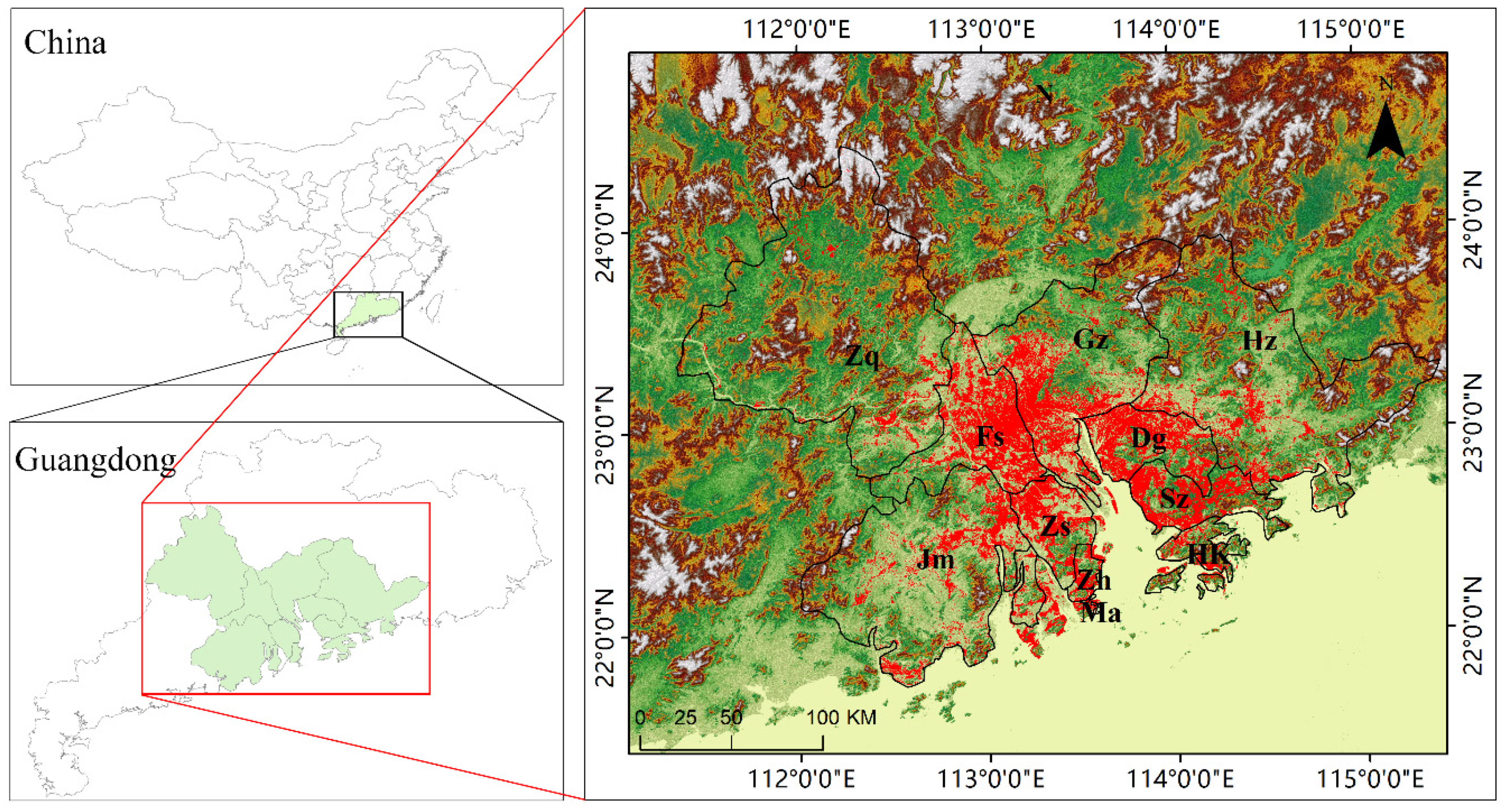
2. Study Area and Data

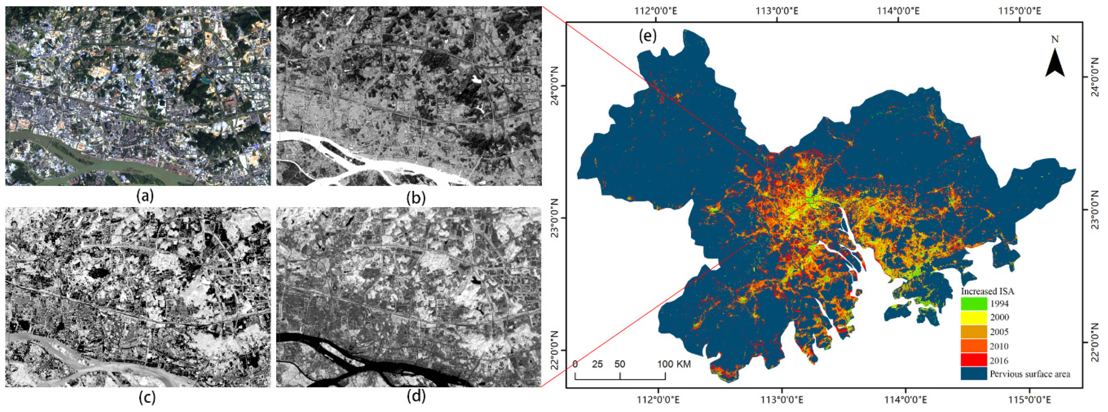
2.1. Study Area

In 1994, the government of Guangdong Province established the Pearl River Delta (PRD) economic zone. By 2014, the urban agglomeration of the GHM Bay Area had become one of the most densely urbanized regions in China, with an urbanization rate of 84.12%. This growth was due to unprecedented urbanization over the previous three decades. The study area is located between 21°30′–23°40′ N and 112°12′–113°48′ E and has a subtropical monsoon climate. The mean annual temperature is 21–23 °C, and annual precipitation totals 1500–2000 mm. The major cities in the region include Guangzhou, Shenzhen, Dongguan, the special administrative region of Hong Kong, and Macau. Economically, the GDP of the GHM Bay Area was 311.8 billion RMB, accounting for 9.83% of China’s GDP, in 2016, with an annual growth rate of 95.6%. In addition, in 2016, 58.74 million people lived in the GHM Bay Area, which constituted 4% of the total population of China at that time (Figure 1).

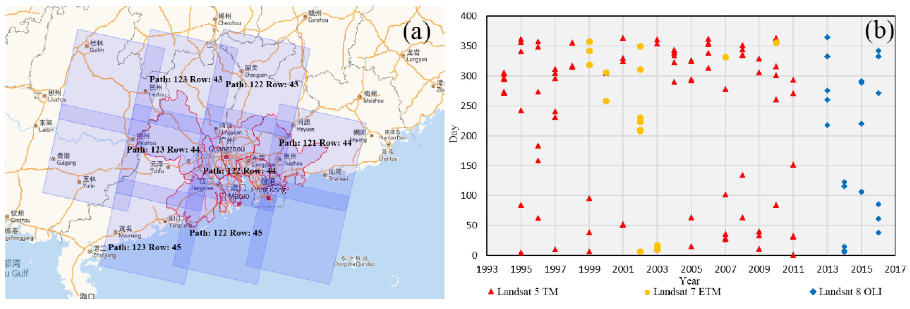
2.2. Data and Preprocessing

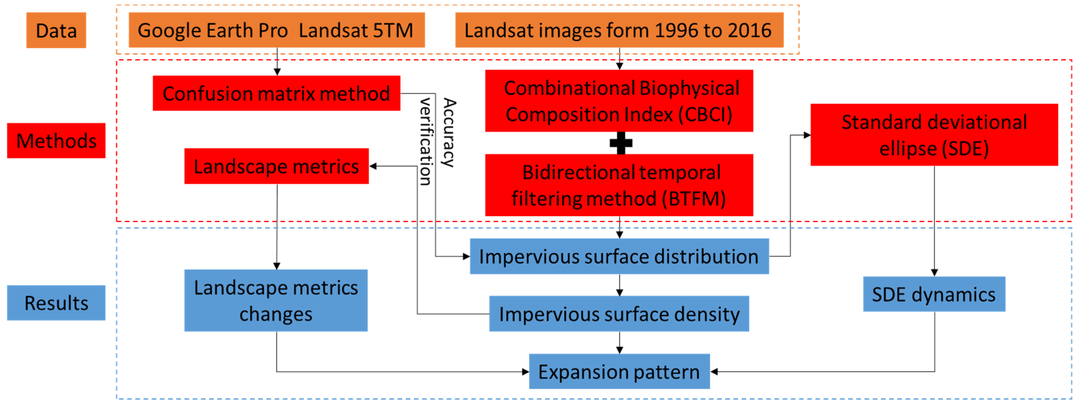
In this study, 161 images (cloud coverage less than 10%) were collected to cover the study area between 1994 and 2016. Note that the impervious surfaces map of 2012 was missing due to a faulty sensor on the Landsat 7 satellite. All the images included the Landsat 5 TM, Landsat 7 ETM+ and Landsat 8 OLI products. These images were downloaded through the United States Geological Survey (USGS) Earth Explorer online portal (see Figure 2). Geometric and orthographic corrections were performed on the acquired images, and the images were rectified to zone 49 of the Universal Transverse Mercator (UTM) projection. Furthermore, all bands of the remote sensing images used in this study were clipped to the study area boundary. Moreover, to remove the effects of scattering and absorption on the used images and to enhance the contrast between impervious surfaces and the soil, radiometric calibration, and atmospheric correction were performed for each image [38,39]. The digital numbers (DNs) of all bands were converted to reflectance values. The conversion parameters were obtained from the respective metadata files that were downloaded with the satellite data. In addition, the high-resolution images incorporated in Google Earth Pro from 2000 to 2016 were obtained to collect ground truth and examine the extraction accuracy of impervious surface maps.

3. Method

3.1. Mapping Impervious Surfaces in the GHM Bay Area

3.1.1. Combinational Biophysical Composition Index (CBCI)

The CBCI was proposed by Zhang et al. [40], which can be used to highlight impervious surfaces, vegetation, water, and bare soil. Moreover, it has better performance than other spectral indices, especially in the GHM Bay Area. The CBCI is defined as follows:

$$\mathrm{CBCI}=\left(A+1\right)\ast \mathrm{MBSI}-\mathrm{OSAVI}+A$$

(1)

where A is a correction factor, in this study, 0.51 was selected as the optimal value to enhance the discrimination of impervious surfaces, bare soil, vegetation, and water. The modified bare soil index (MBSI) can be used to distinguish bare soil from other land cover types, and it is calculated using the following equation:

$$\mathrm{MBSI}=\frac{\left(\mathsf{\rho }\mathrm{Red}-\mathsf{\rho }\mathrm{Green}\right)\ast 2}{\mathsf{\rho }\mathrm{Red}+\mathsf{\rho }\mathrm{Green}-2}$$

(2)

where $\mathsf{\rho }\mathrm{Red}$ and $\mathsf{\rho }\mathrm{Green}$ are the reflectance values of the red and green bands, respectively, and 2 is a correction factor that can be used to enhance the distinction of bare soil and the other three biophysical compositions. The optimized soil adjusted vegetation index (OSAVI) was developed by Rondeaux in 1996 [41]. After the CBCI was calculated, the Kirtler Illingworth (KI) method [42] was employed to obtain an optimal threshold and produce a binary map of impervious surfaces.

3.1.2. Bidirectional Temporal Filtering Method (BTFM)

After the time series of impervious surface images were acquired, a bidirectional temporal filtering method (BTFM) was applied to correct misclassified pixels and improve accuracy [43]. This method is based on the hypothesis that impervious surfaces do not revert back to vegetation or bare soil in a short time period after they are converted from vegetation or bare soil. The impervious surface image from 2002 was selected as the starting image because it was extracted by the Landsat 7 TM images and has relatively high accuracy. Moreover, the year 2002 at the middle part of the study period. The annual impervious surface maps were reset as {${\mathrm{M}}_1$, …, ${\mathrm{M}}_{i-1}, {\mathrm{M}}_i, {\mathrm{M}}_{i+1}$, …, ${\mathrm{M}}_t$} where t was the year and ${\mathrm{M}}_i$ was the impervious surface image of 2002. If a pixel was classified as a pervious surface in ${\mathrm{M}}_i$ and ${\mathrm{M}}_{i+2}$ but was an impervious surface in ${\mathrm{M}}_{i+1}$, the pixel in ${\mathrm{M}}_{i+1}$ would first be set as an uncertain pixel. Moreover, if that pixel was classified as a pervious surface in ${\mathrm{M}}_{i-2}$ and if the pixel in ${\mathrm{M}}_{i-1}$ was also identified as an uncertain pixel, then the pixels in ${\mathrm{M}}_{i+1}$ and ${\mathrm{M}}_{i-1}$ would both be corrected as pervious surfaces, rather than impervious surfaces. Then, a moving window was applied to the time series beginning bidirectionally at ${\mathrm{M}}_{i-1}$ and ${\mathrm{M}}_{i+1}$ and proceeding annually to ${\mathrm{M}}_{i-2}$ and ${\mathrm{M}}_{i+2}$.

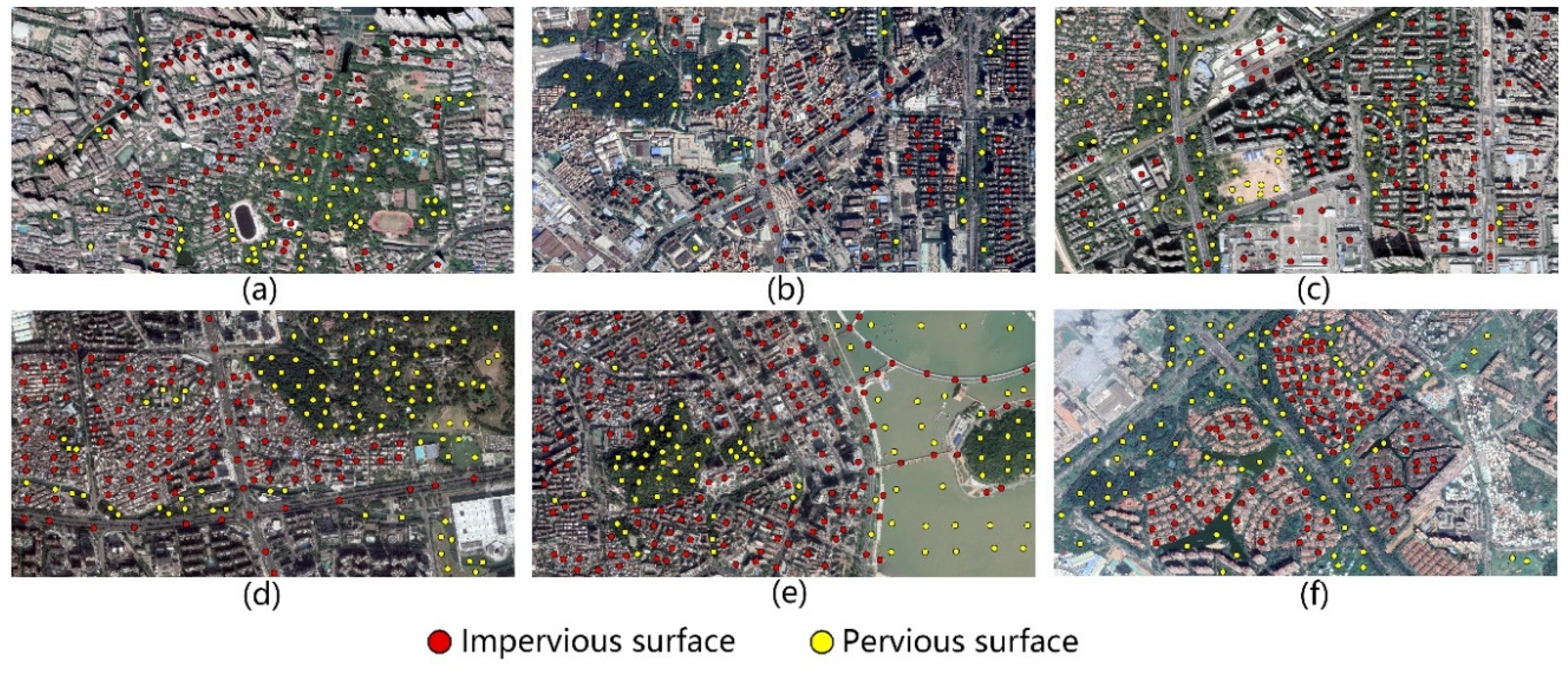
3.1.3. Mapping Accuracy Verification

The high-resolution images incorporated in Google Earth Pro and the Landsat 5 TM images were used to assess the accuracies of the ISA maps. The “view historical imagery” tool in Google Earth Pro was used to find the best possible referenced image from 2000 to 2016. Before 2000, the verification samples were acquired by the Landsat 5 TM images. This study randomly selected 200 verification sample points per year in each city of the GHM Bay Area (Figure 3). Moreover, a confusion matrix method was used to verify the accuracy of the ISA extraction results.

3.2. Calculation of Impervious Surface Density

To analyze the dynamics of the impervious surface density, the ISA images were resized to 100 × 100 m cells, and the ISA proportion was calculated in areas of 1 km². The equation used to calculate the impervious surface density is:

$$ISD=\frac{{{\displaystyle \sum }}_{i=1}^{10}{a}_i}{1000}\times 100\%$$

(3)

where ISD is impervious surface density in 1 km², if cell $i$ is impervious surface a = 100, else a = 0.

3.3. Analysis of the Changes in Landscape Metrics

Landscape metrics provide a quantitative description of the composition and configuration of urban landscapes [44,45]. In this study, these metrics were employed to compute the degree of expansion of the ISA at different ISA density levels; this analysis was conducted using FRAGSTATS 4.2 with the eight-neighbor rule. Based on the objectives of this study and to avoid redundancy, ISA expansion was characterized by six prominent spatial metrics that are widely used to investigate urban expansion and its effect on the environment. These spatial metrics included the number of patches (NP), patch density (PD), largest patch index (LPI), landscape shape index (LSI), mean patch size (AREA_MN), and aggregation index (AI) (

Table 1. Landscape metrics used in this study.

Landscape Metric	Calculation and Description
Number of patches (NP)	$\mathrm{NP}=n_i$ where $n_i$ is the number of patches of patch type (class) i in the landscape.
Patch density (PD)	$\mathrm{PD}=\frac{n_i}{A}\left(\mathrm{10,000}\right)\left(100\right)$ where $n_i$ is the number of patches of patch type (class) i in the landscape and A is the total landscape area (m2).
Largest patch index (LPI)	$\mathrm{LPI}=\frac{\begin{array}{c}n\\ \underset{j=1}{\max }\left(a_{ij}\right)\end{array}}{A}\left(100\right)$ where $a_{ij}$ is the area (m2) of patch ij and A is the total landscape area (m2).
Landscape shape index (LSI)	$\mathrm{LSI}=\frac{0.25{{\displaystyle \sum }}_{k=1}^m{e}_{ik}^{*}}{\sqrt{A}}$ where $e_{ik}^{*}$ is the total length (m) of the edge in the landscape between patch types (classes) i and k; this includes the entire landscape boundary and some or all background edge segments involving class i.
Mean patch size (AREA_MN)	$\mathrm{AREA}\text{\_}\mathrm{MN}=\frac{1}{\mathrm{10,000}/n}{\displaystyle \sum _{i=1}^n}{x}_i$ where n is the number of patches and $x_i$ is the area of patch i.
Aggregation index (AI)	$\mathrm{AI}=\left[\frac{g_{ii}}{\max \to g_{ii}}\right]\left(100\right)$ where $g_{ii}$ is the number of like adjacencies (joins) between pixels of patch type (class) i based on the single-count method and $\max \to g_{ii}$ is the maximum number of like adjacencies (joins) between pixels of patch type (class) i based on the single-count method.

). The ISA density changes at different levels were analyzed using these landscape metrics.

3.4. Standard Deviational Ellipse (SDE)

In this study, we used the SDE [46] method to further measure the orientation, direction, and spatiotemporal developmental trends of ISA expansion. For each ISA image, four parameters of the SDE (i.e., ellipse center, long axis, short axis, and azimuth) were calculated. The ellipse center of the SDE is gravity center. The azimuth of the SDE is calculated as follows:

$$\tan \theta =\frac{\left({{\displaystyle \sum }}_{i=1}^n{\omega }_i^2{\tilde{x}}_i^2-{{\displaystyle \sum }}_{i=1}^n{\omega }_i^2{\tilde{y}}_i^2\right)+\sqrt{{\left({{\displaystyle \sum }}_{i=1}^n{\omega }_i^2{\tilde{x}}_i^2-{{\displaystyle \sum }}_{i=1}^n{\omega }_i^2{\tilde{y}}_i^2\right)}^2-4{\left({{\displaystyle \sum }}_{i=1}^n{\omega }_i^2{\tilde{x}}_i{\tilde{y}}_i\right)}^2}}{2{{\displaystyle \sum }}_{i=1}^n{\omega }_i^2{\tilde{x}}_i{\tilde{y}}_i},$$

(4)

$$\{\begin{array}{l}{\tilde{x}}_i=x_i-\overline{x}\\ {\tilde{y}}_i=y_i-\overline{y}\end{array},$$

(5)

where $\theta$ is the azimuth of the ellipse, indicating the angle measured clockwise from north to the long axis of the ellipse; $x_i$ and $y_i$ are the deviations between the $i$th grid center and the gravity center in the $x$ and $y$ directions, respectively, and ${\omega }_i$ is the weight. In this study, the weight ${\omega }_i$ represents the impervious surface fraction of the $i$th grid. The standard deviations ${\sigma }_x$ and ${\sigma }_y$ of the ellipse in the $x$ and $y$ directions, respectively, are calculated as follows.

$$\{\begin{array}{l}{\sigma }_x=\sqrt{\frac{{{\displaystyle \sum }}_{i=1}^n{\left({\omega }_i{\tilde{x}}_i\cos \theta -{\omega }_i{\tilde{y}}_i\sin \theta \right)}^2}{{{\displaystyle \sum }}_{i=1}^n{\omega }_i^2}}\\ {\sigma }_y=\sqrt{\frac{{{\displaystyle \sum }}_{i=1}^n{\left({\omega }_i{\tilde{x}}_i\sin \theta -{\omega }_i{\tilde{y}}_i\cos \theta \right)}^2}{{{\displaystyle \sum }}_{i=1}^n{\omega }_i^2}}\end{array}$$

(6)

The long axis, short axis, and azimuth represent the developmental trends of the ISA and the development direction. The ratio of the long axis to the short axis denotes the degree of aggregation or dispersion of the ISA. If this ratio is greater than 1, the ISA is characterized by obvious orientational effects. However, a ratio equal to 1 indicates no directional characteristics. In this study, an SDE of one ISA image was determined based on the SDE parameters, which were used to reveal whether the spatial distribution of the impervious surface was elongated; additionally, the SDE reflected the particular orientation of an impervious surface (Figure 4).

4. Results

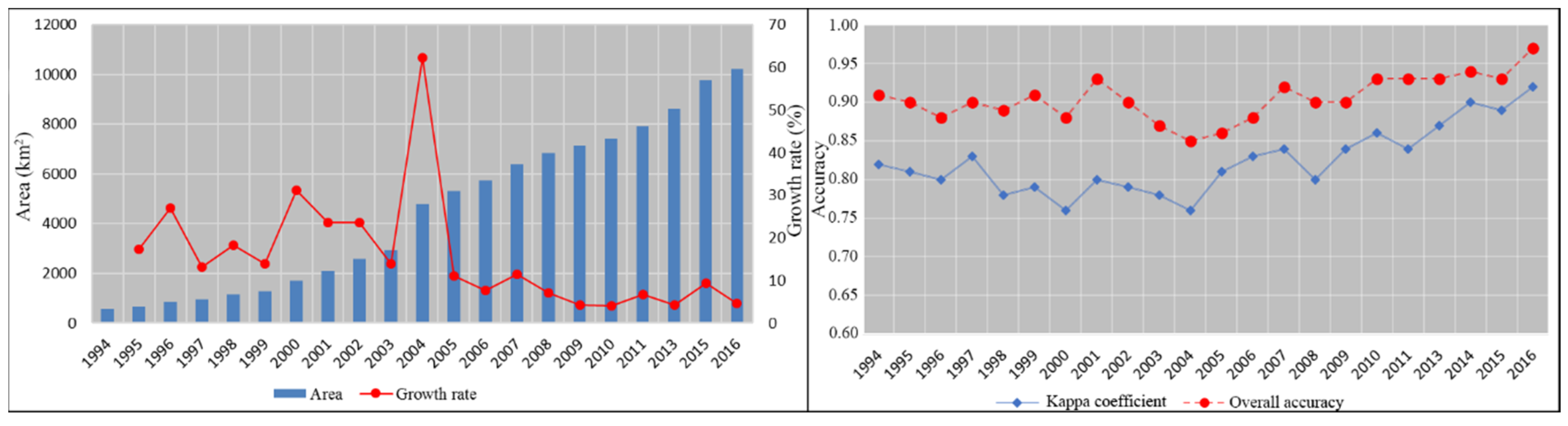
4.1. Mapping Accuracy and Impervious Surface Dynamics

The results of the accuracy verification are shown in Figure 5 (right). The average overall accuracy and Kappa coefficient of the impervious surface maps from 1994 to 2016 were 0.91 and 0.83, respectively. The relatively low accuracies of the results from 1994 to 2008 were due to the effects of cloud cover and low image quality; thus, the average overall accuracy was 0.89, and the Kappa coefficient was 0.8. In addition, the impervious surface images from 2009 to 2016 had relatively higher accuracies; the mean overall accuracy was 0.94, and the Kappa coefficient was 0.88 (see Figure 5, right). The dynamic changes in the ISA from 1994 to 2016 are presented in Figure 5 (left), which shows the different spatial patterns over the past two decades. Overall, the impervious surfaces of the GHM Bay Area rapidly expanded from 569.23 km² in 1994 to 10,200.53 km² in 2016, with an average annual growth rate of 51.7%. Moreover, the ISA represented 0.9% of the total area of the GHM Bay Area in 1994. However, it accounted for 17% of the total area of the GHM Bay Area in 2016. In 1994, most impervious surfaces were aggregated in Guangzhou, Shenzhen, and Hong Kong. After 1999, the expansion of impervious surfaces increased rapidly. With the fast urbanization process, a new urban core appeared in Foshan, which is located in the southwestern region of Guangzhou. Then, another urban core emerged in Dongguan in 2006, which is located in the southeastern region of Guangzhou. Furthermore, the expansion of impervious surfaces in Dongguan and Shenzhen mainly occurred along the Pearl River and the coastline of the GHM Bay Area.

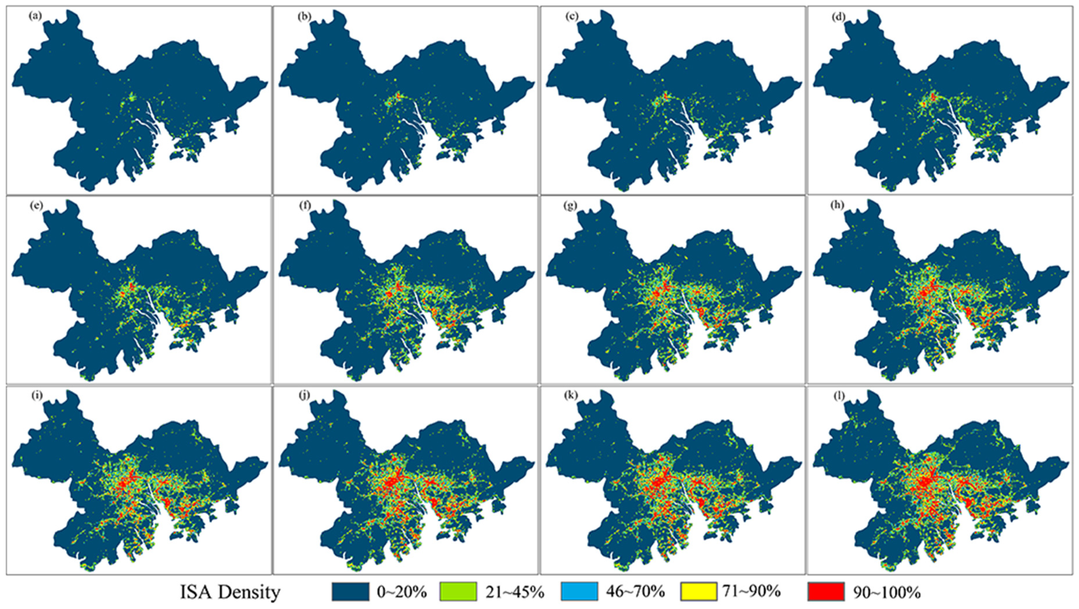
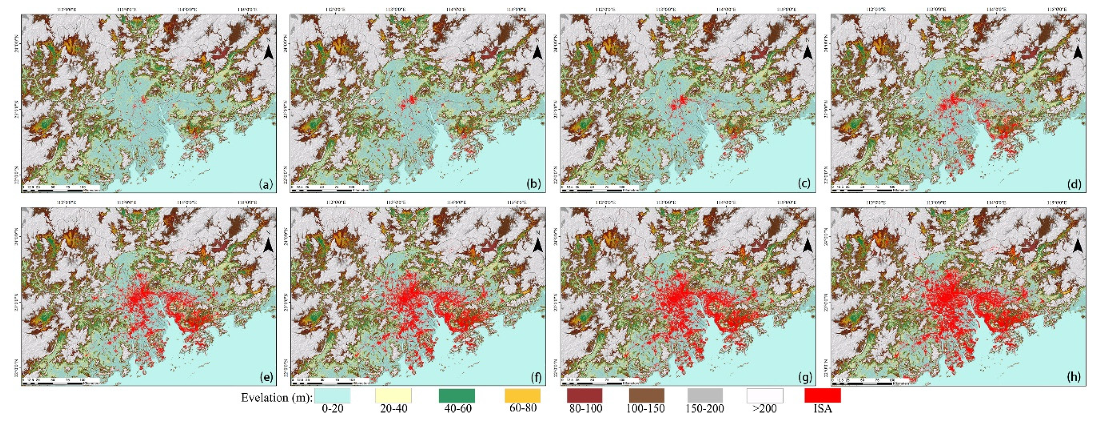
4.2. Impervious Surface Density Distribution and Dynamics

The ISA density in the GHM Bay Area was grouped into five levels: pervious surface area (ISA density less than 20%), low-density area (ISA density between 21% and 45%), medium-density area (ISA density between 46% and 70%), high-density area (ISA density between 71% and 90%) and very high-density area (ISA density higher than 90%). As shown in Figure 6 and Figure 7, the pervious surface area represented a large portion of the GHM Bay Area. However, the very high-density and high-density areas were aggregated in the urban core areas of Guangdong, Foshan, Shenzhen, and Hong Kong in 1994. Moreover, the very high-density area increased with rapid urban expansion. In 2000, most very high-density and high-density areas were located in Guangdong and Foshan. Furthermore, the medium-density and low-density areas were distributed along the Pearl River and the coastline in Dongguan and Shenzhen. From 2001 to 2008, the very high-density area increased rapidly in Guangzhou, Foshan, Dongguan, and Shenzhen. Between 2009 and 2016., the very high-density area displayed a slow expansion rate. However, the high-density area grew rapidly in the GHM Bay Area.

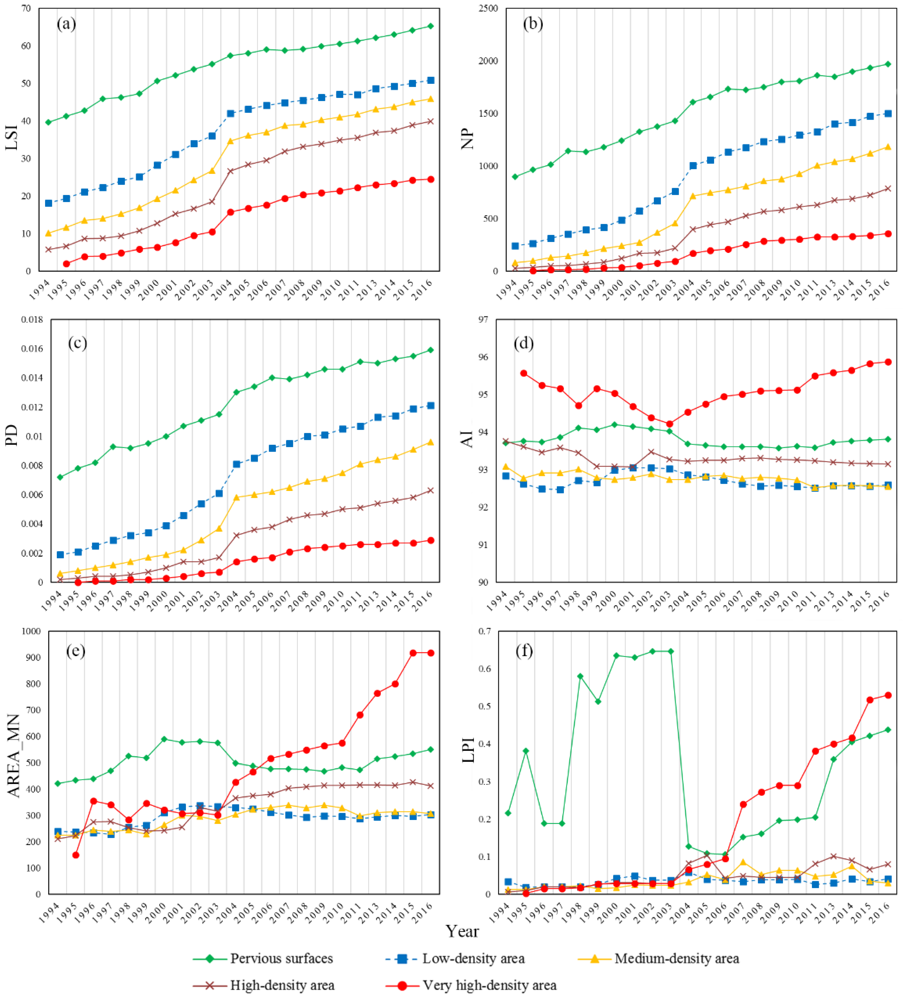
4.3. Landscape Metrics Dynamics for Different ISA Density Groups

The dynamics of six different landscape metrics for five ISA density groups over the entire study period are depicted in Figure 8. Note that the ISA in 1994 has only four ISA density groups except very high-density area, due to the small quantity and limited dispersion of ISAs in 1994. The LSI, NP, and PD displayed similar increasing trends between 1994 and 2016 (see Figure 8a–c). Pervious surfaces exhibited the highest values, followed by the low-density area, the medium-density area, and the high-density area. Furthermore, the very high-density area displayed the lowest values from 1994 to 2016. For the landscape metric AI (see Figure 8d), the very high-density area still exhibited the highest values, with a minimum observed in 2004. Previous surfaces displayed the second-highest AI values from 1994 to 2016, followed by those of the high-density area. However, the low-density area and the medium-density area had approximately the same AI values, especially after 2011. The AREA_MN trend of each ISA density group (see Figure 8e) indicated that the value of the very high-density area increased rapidly, especially after 2004. Before 2005, the value of the very high-density area was lower than that of pervious surfaces. Moreover, the value of the low-density area peaked in 2002 and then began to decrease. The value of the medium-density area displayed an overall increasing trend and reached a peak in 2009. In addition, the value of the high-density area increased gradually, and this value was higher than those of the low-density area and the medium-density area after 2003. Figure 8f reveals the dynamics of the LPI for the five ISA density groups. The LPI value of pervious surfaces experienced a drastic change from 1994 to 2004. Notably, it fluctuated between 1994 and 2000 and then decreased sharply from 2003 to 2004. After 2004, the value began to rapidly increase, especially after 2011. The LPI value of the very high-density area increased slowly until 2006 but then sharply increased. In addition, the LPI values of the low-density, medium-density, and high-density areas slightly increased and reached peaks in 2004, 2007, and 2013, respectively.

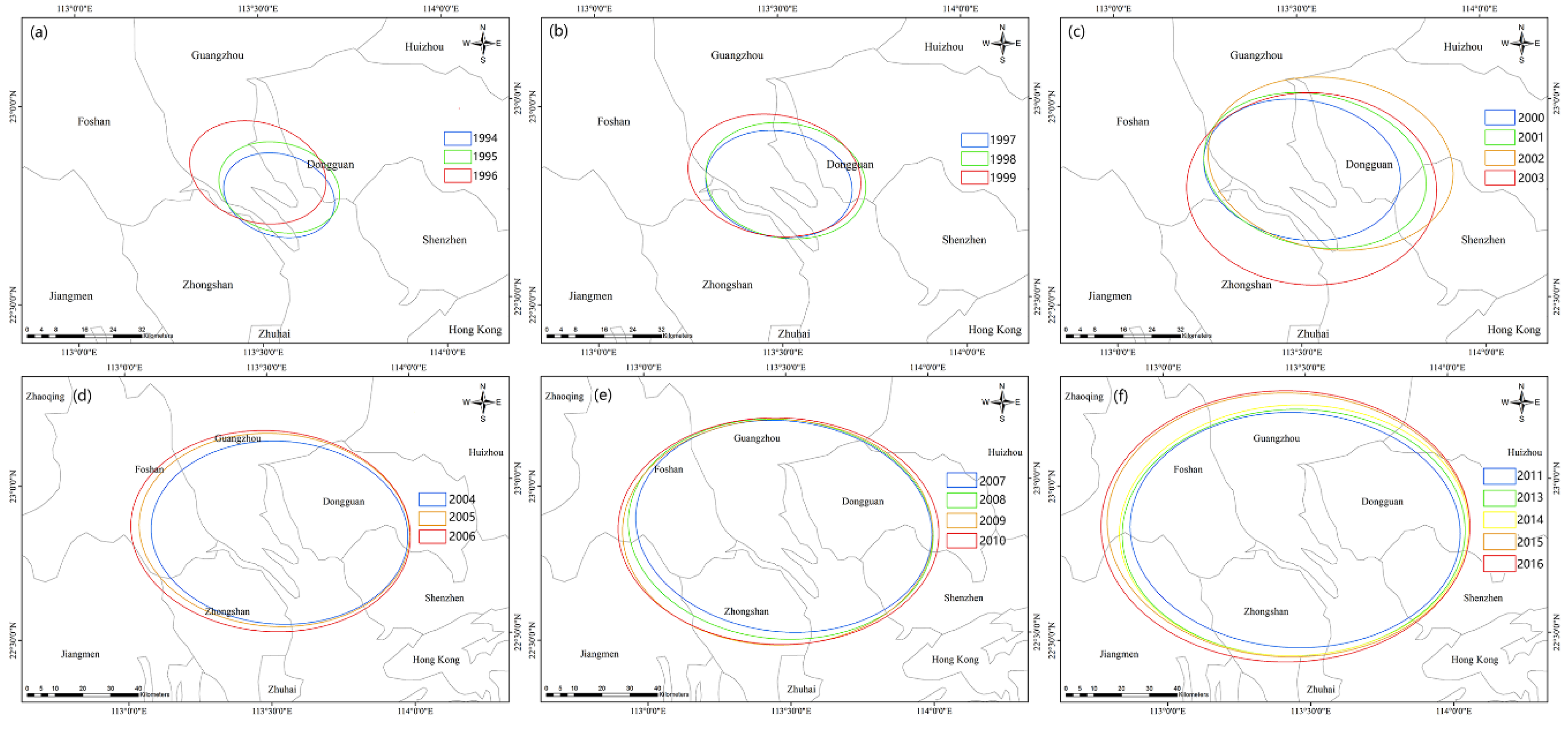
4.4. Impervious Surface Standard Deviational Ellipse (SDE) Dynamics

The SDE was employed to further present the impervious surface dynamics for different orientations and distribution. The SDEs of the impervious surfaces over the entire region from 1994 to 2016 are shown in Figure 9. The detailed parameters of the SDEs are listed in

Table 2. The parameters of the standard deviational ellipses from 1994 to 2016.

Year	Major Axis (m)	Minor Axis (m)	Major Axis/Minor Axis	Orientation (°)
1994	15,818.2	11,454.5	1.38	163.43
1995	17,147.8	12,400.5	1.38	164.92
1996	19,498.4	13,844.5	1.40	162.72
1997	20,633.2	14,814.0	1.39	170.24
1998	22,536.7	16,048.6	1.40	170.55
1999	24,348.6	16,906.0	1.44	170.36
2000	27,749.3	19,469.5	1.43	169.88
2001	31,505.7	21,176.3	1.49	167.43
2002	34,497.4	23,897.5	1.44	170.93
2003	34,959.9	26,876.5	1.30	178.29
2004	46,261.3	32,954.1	1.40	176.45
2005	48,758.2	34,730.8	1.40	175.62
2006	50,425.7	36,145.6	1.39	175.57
2007	53,500.5	37,951.0	1.41	173.55
2008	55,030.2	39,530.7	1.39	174.75
2009	55,872.7	40,605.0	1.38	179.28
2010	57,790.2	40,816.9	1.42	178.43
2011	59,473.9	42,338.2	1.40	177.65
2013	61,764.4	44,378.4	1.39	178.51
2014	62,925.6	45,158.9	1.39	178.05
2015	65,329.3	47,529.9	1.37	178.28
2016	66,457.1	48,857.5	1.36	179.93

. The orientation of the SDE indicates the directional trend of impervious surface expansion. An obvious orientation of SDEs can be found in Figure 9, and this orientation changed in different periods. From 1994 to 1999, the orientation changed from 163.43° to 170.36°, but it then decreased from 170.36° in 1999 to 167.43° in 2001. After 2001, the orientation gradually increased from 170.93° in 2002 to 179.93° in 2016, representing an average annual angle increase of 0.643°. Before 2008, the spatial direction of impervious surface expansion was from the northwest to the southeast; however, after 2008, the orientation of the impervious surface growth was from the west to the east.

The major axis, the minor axis, and their ratio indicate the spatial distribution of the ISA. If the ratio is close to 1, the impervious surfaces have an uncertain principal direction of expansion. Meanwhile, the ISA is distributed discretely in a region. Table 2 shows that the ratio fluctuated between 1.36 and 1.49 from 1994 to 2016. The ratio was increased from 1996 to 2001 with the highest ratio of 1.49 in 2001. The lowest ratio appeared in 2003 with a value of 1.30. During this period, the ISA was rapidly expanded around the urban area. Farmlands, water bodies, and open spaces were replaced by impervious surfaces. Moreover, the ratio showed a decreased trend from 2004 to 2016 with a relatively low value of 1.36. In this stage, the cities were restricted from expanding to the surrounding areas. Moreover, old urban landscapes and open spaces were redeveloped. These results indicated that the expansion of ISA had an explicit orientation from 1994 to 2003. However, the sprawl direction of ISA was less obvious from 2004 to 2016. In addition, the spatial distribution of the ISA was changed from aggregation to dispersion due to the rapid urban development.

5. Discussion

5.1. ISA Expansion Modes in Different Periods

The results presented above illustrated that the ISA experienced rapid expansion in the GHM Bay Area. However, the growth rates are decreased from 1994 to 2016. The ISA sprawl results are consistent with other studies [36,43,47]. Moreover, the analysis results indicate that the ISA in the GHM Bay Area experienced different growth patterns.

From 1994 to 2004, the values of LSI, NP, and PD of ISA showed a slowly increasing trend. However, the value of AI has a decreased trend in ISA. The high values of NP and PD and low values of AI suggested a more scattered pattern of ISA in the GHM Bay Area [48]. Notably, the previous surface area and low-density area have relatively high slopes of NP and PD. It indicated that the ISA was mainly expanded in previous surface and low-density areas. In addition, the average ratio of SDEs was 1.40 before 2004. Moreover, the highest value of the ratio was 1.49 in 2001. The changing pattern of landscape metrics and high ratio of SDEs indicated that the impervious surfaces were sprawled into suburban areas from the northwest to the southeast due to the expansion mode of edge expanding and leapfrogging. In this stage, water bodies, open spaces, and farmlands around the urban area were used to build residential areas, commercial areas, industrial parks, and other infrastructure. Therefore, a new urban core was developing in Foshan [47]. Furthermore, the increases in high-density area and low-density area alongside a decrease in paddy fields in the coastal hinterlands are the most prominent changes in this urban expansion pattern.

From 2005 to 2016, the ISA development pattern in the GHM Bay Area was changed. Infilling and consolidation replaced edge expanding and leapfrogging as the primary development pattern. Note that the value of AI was increased rapidly, especially in a very high-density area. The increased value of AI indicated that the impervious surfaces were aggregated in the GHM Bay Area because of infilling and consolidation. In addition, the slops of NP and PD between 2004 and 2016 were lower than that between 1994 and 2003 in very high-density and high-density areas. The lower slopes indicated that the number of ISA patches decreased due to infilling and consolidation development patterns. Meantime, this development pattern caused the less obvious orientation of urban expansion. Thus, the average ratio of SEDs from 2006 to 2016 was 1.39, which was lower than the average ratio from 1994 to 2005. During this period, the infilling of open space inside urban areas and the redevelopment of the old urban landscape were the main urban development patterns [49]. Although the growth rate of ISA was decreased, the high-density area still had a rapid sprawl trend (Figure 5). Therefore, the ISA formed a whole area in Guangzhou and Foshan (Figure 7). Moreover, the widely distributed ISA led to the relatively low ratios of SDEs from 2004 to 2016.

5.2. Driving Forces of the ISA Expansion Modes

Economic and population growth are the driving forces of urban development [50]. Generally, rapid economic and population growth are accompanied by obvious ISA expansion. Since the Guangdong government established the “PRD economic zone” in 1994, the GHM Bay Area has experienced rapid socioeconomic development. Furthermore, China joined the World Trade Organization (WTO) in 2001, the population and economic growth was accelerated by globalization, especially in the coastal zone of China [51,52]

Previous research has shown that topography is an important factor that can constrain urban expansion and affect development patterns [53]. Figure 10 illustrated that the development space of Guangzhou is limited by the mountains to the northeast and east. The ISA expansion in Foshan and Zhongshan is restricted by the river and mountainous region to the west. In addition, the ISA in Shenzhen and Hong Kong is mainly aggregated along the coastline of the GHM Bay Area. Moreover, the ISA is restricted by the mountainous area east of Shenzhen and Hong Kong. Therefore, the ISA growth pattern of the GHM Bay Area changed from edge expanding and leapfrogging to infilling and consolidation after 2005. This can be explained by the fact that not so much open arable and bare land is available for development due to the large areas of water bodies and mountainous areas [36].

Policy is another significant factor that can affect urban development patterns. Guangdong province, an “important window” of the reform and opening-up policy in China, established the PRD economic zone in 1994. The central and local governments have issued a series of policies to support the economic and urban development of Guangdong province. Therefore, the ISA of the GHM Bay Area was rapidly sprawled around the urban areas. From 2000 to 2010, the government has begun implementing the policy of “building an ecological civilization, basically forming the industrial structure, growth mode, and consumption mode that save energy and resources and protect the ecological environment” proposed in the 17th National Congress of the Communist Party of China, and has maintained a good balance between high-speed urbanization and ecological resource protection. In 2009, the Ministry of Land and Resources of the People’s Republic of China implemented an “arable land minimum” policy to protect prime farmland. From 2010 to 2018, the release of the Implementation Plan of the National Ecological Civilization Construction Demonstration Zone in the GHM Bay Area [49]. During this period, the farmland and ecological land were protected by those policies, which caused an infilling and consolidation growth pattern of GHM Bay Area.

5.3. Recommendations for Future Urban Development

Previous studies have demonstrated that the high-density ISA area can cause various urban environmental problems, especially when the ISA density is higher than 90%. These problems include things such as runoff increase, water pollution, and urban heat islands (UHIs) [54,55,56]. The study area has relatively high precipitation during the rainy season. Particularly, the storm can cause the disaster of urban waterlogging in the high-density ISAs. Moreover, the flood takes pollutants from impervious surfaces to streams and water bodies, which caused the degradation of water quality. The ISA of the GHM Bay Area experienced a drastic expansion from 569.23 km² in 1994 to 10,200.53 km² in 2016. Additionally, the infilling and consolidation mode of ISA growth made the high-density ISA area expand rapidly after 2005. Based on the aims of environmental protection and urban sustainable development, this study proposes some options for future urban development: (1) for future urban construction, the low-impact development (LID) approach should be considered during the process of urbanization; additionally, (2) the old city districts should be reconstructed to increase the proportion of vegetation and decrease the density of ISA, (3) the new urban core should be established in a suitable area to further mitigate the ISA density.

6. Conclusions

Different urban growth patterns have various impact degrees on the urban ecosystem and environment. Impervious surface, a typical artificial construction can be used to reflect urban development. Therefore, this study documented the ISA growth pattern of GHM Bay Area changed from edge expanding to infilling and consolidation with a turning point in 2004. The time series of impervious surface images revealed that the ISA of the GHM Bay Area experienced a drastic expansion from 569.23 km² in 1994 to 10,200.53 km² in 2016, with an average annual growth rate of 51.7%. In addition, an analysis of the distribution and dynamics of the ISA density indicated that the very high-density and high-density areas rapidly expanded and were mainly located in the urban core areas. The results of landscape metrics and SDEs indicated that the ISA growth pattern changed from edge expanding and leapfrogging to infilling and consolidation, with a turning point in 2004. Moreover, the principal sprawl orientation of the ISA was northwest to southeast before 2004. After 2004, the expansion direction of the ISA was less obvious due to the development pattern of infilling and consolidation. The rapid increase of GDP and population are the driving forces of urban expansion. However, topography and ecological protection policies as the limiting factors, which caused the infilling of the inner city and redevelopment of old urban areas.

Similarly, the expansion patterns of other urban agglomerations and megacities are changed with rapid urbanization. Thus, the urban ecosystem and environment of those regions are also influenced by the different growth patterns. This method can be applied to other regions by using time-series remote sensing images. The landscape metrics and SDE can be used to identify the ISA growth pattern as well as recognition of turning points with time-series images.

References

1. American Association for the Advancement of Science. Rise of the City. Science 2016, 352, 906. [Google Scholar] [CrossRef] [PubMed]
2. Dos Santos, A.R.; de Oliveira, F.S.; da Silva, A.G.; Gleriani, J.M.; Gonçalves, W.; Moreira, G.L.; Silva, F.G.; Branco, E.R.F.; Moura, M.M.; da Silva, R.G.; et al. Spatial and temporal distribution of urban heat islands. Sci. Total Environ. 2017, 605–606, 946–956. [Google Scholar] [CrossRef] [PubMed]
3. Laaidi, K.; Zeghnoun, A.; Dousset, B.; Bretin, P.; Vandentorren, S.; Giraudet, E.; Beaudeau, P. The Impact of Heat Islands on Mortality in Paris during the August 2003 Heat Wave. Environ. Health Perspect. 2012, 120, 254–259. [Google Scholar] [CrossRef] [PubMed] [Green Version]
4. Yang, J.; Zhang, Z.; Li, X.; Xi, J.; Feng, Z. Spatial differentiation of China’s summer tourist destinations based on climatic suitability using the Universal Thermal Climate Index. Theor. Appl. Climatol. 2018, 134, 859–874. [Google Scholar] [CrossRef]
5. Weng, Q. Remote sensing of impervious surfaces in the urban areas: Requirements, methods, and trends. Remote Sens. Environ. 2012, 117, 34–49. [Google Scholar] [CrossRef]
6. Xian, G.; Crane, M. Assessments of urban growth in the Tampa Bay watershed using remote sensing data. Remote Sens. Environ. 2005, 97, 203–215. [Google Scholar] [CrossRef]
7. Paul, M.J.; Meyer, J.L. Streams in the urban landscape. Annu. Rev. Ecol. Syst. 2001, 32, 333–365. [Google Scholar] [CrossRef]
8. Yang, K.; Yang, Y.; Zhu, Y.; Li, C.; Meng, C. Social and economic drivers of PM2.5 and their spatial relationship in China. Geogr. Res. 2016, 35, 1051–1060. [Google Scholar]
9. Touchaei, A.G.; Akbari, H.; Tessum, C.W. Effect of increasing urban albedo on meteorology and air quality of Montreal (Canada)—Episodic simulation of heat wave in 2005. Atmos. Environ. 2016, 132, 188–206. [Google Scholar] [CrossRef]
10. Mou, B.; He, B.-J.; Zhao, D.-X.; Chau, K.-w. Numerical simulation of the effects of building dimensional variation on wind pressure distribution. Eng. Appl. Comput. Fluid Mech. 2017, 11, 293–309. [Google Scholar] [CrossRef]
11. Kim, H.; Jeong, H.; Jeon, J.; Bae, S. The Impact of Impervious Surface on Water Quality and Its Threshold in Korea. Water 2016, 8, 111. [Google Scholar] [CrossRef] [Green Version]
12. Tong, S.T.; Chen, W. Modeling the relationship between land use and surface water quality. J. Environ. Manag. 2002, 66, 377–393. [Google Scholar] [CrossRef] [PubMed]
13. Zhou, D.; Zhao, S.; Liu, S.; Zhang, L.; Zhu, C. Surface urban heat island in China’s 32 major cities: Spatial patterns and drivers. Remote. Sens. Environ. 2014, 152, 51–61. [Google Scholar] [CrossRef]
14. Zhao, Z.-Q.; He, B.-J.; Li, L.-G.; Wang, H.-B.; Darko, A. Profile and concentric zonal analysis of relationships between land use/land cover and land surface temperature: Case study of Shenyang, China. Energy Build. 2017, 155, 282–295. [Google Scholar] [CrossRef]
15. Arnold, C.L.; Gibbons, C.J. Impervious Surface Coverage: The Emergence of a Key Environmental Indicator. J. Am. Plan. Assoc. 1996, 62, 243–258. [Google Scholar] [CrossRef]
16. Pal, M.; Mather, P.M. An assessment of the effectiveness of decision tree methods for land cover classification. Remote Sens. Environ. 2003, 86, 554–565. [Google Scholar] [CrossRef]
17. Yan, Y.; Zhang, C.; Hu, Y.; Kuang, W. Urban land-cover change and its impact on the ecosystem carbon storage in a dryland city. Remote Sens. 2016, 8, 6. [Google Scholar] [CrossRef] [Green Version]
18. Shao, Z.; Liu, C. The integrated use of DMSP-OLS nighttime light and MODIS data for monitoring large-scale impervious surface dynamics: A case study in the Yangtze River Delta. Remote Sens. 2014, 6, 9359–9378. [Google Scholar] [CrossRef] [Green Version]
19. Deng, C.; Wu, C. A spatially adaptive spectral mixture analysis for mapping subpixel urban impervious surface distribution. Remote Sens. Environ. 2013, 133, 62–70. [Google Scholar] [CrossRef]
20. Somers, B.; Asner, G.P.; Tits, L.; Coppin, P. Endmember variability in spectral mixture analysis: A review. Remote Sens. Environ. 2011, 115, 1603–1616. [Google Scholar] [CrossRef]
21. Wang, L.; Sousa, W.P.; Gong, P.; Biging, G.S. Comparison of IKONOS and QuickBird images for mapping mangrove species on the Caribbean coast of Panama. Remote Sens. Environ. 2004, 91, 432–440. [Google Scholar] [CrossRef]
22. Benz, U.C.; Hofmann, P.; Willhauck, G.; Lingenfelder, I.; Heynen, M. Multi-resolution, object-oriented fuzzy analysis of remote sensing data for GIS-ready information. ISPRS J. Photogramm. Remote Sens. 2004, 58, 239–258. [Google Scholar] [CrossRef]
23. Van de Voorde, T.; De Genst, W.; Canters, F.; Stephenne, N.; Wolff, E.; Binard, M. Extraction of land use/land cover related information from very high resolution data in urban and suburban areas. Remote Sens. Transit. 2004, 01, 237–244. [Google Scholar]
24. Estoque, R.C.; Murayama, Y. Classification and change detection of built-up lands from Landsat-7 ETM+ and Landsat-8 OLI/TIRS imageries: A comparative assessment of various spectral indices. Ecol. Indic. 2015, 56, 205–217. [Google Scholar] [CrossRef]
25. Gong, J.; Hu, Z.; Chen, W.; Liu, Y.; Wang, J. Urban expansion dynamics and modes in metropolitan Guangzhou, China. Land Use Policy 2018, 72, 100–109. [Google Scholar] [CrossRef]
26. Li, C.; Li, J.; Wu, J. Quantifying the speed, growth modes, and landscape pattern changes of urbanization: A hierarchical patch dynamics approach. Landsc. Ecol. 2013, 28, 1875–1888. [Google Scholar] [CrossRef]
27. Pham, H.M.; Yamaguchi, Y.; Bui, T.Q. A case study on the relation between city planning and urban growth using remote sensing and spatial metrics. Landsc. Urban Plan. 2011, 100, 223–230. [Google Scholar] [CrossRef]
28. Yang, K.; Zhang, S.; Luo, Y.; Xu, Q.; Qu, L. The widening urbanization gap between the Three Northeast Provinces and the Yangtze River Delta under China’s economic reform from 1984 to 2014. Int. J. Sustain. Dev. World Ecol. 2017, 25, 262–275. [Google Scholar] [CrossRef]
29. Xu, J.; Zhao, Y.; Zhong, K.; Zhang, F.; Liu, X.; Sun, C. Measuring spatio-temporal dynamics of impervious surface in Guangzhou, China, from 1988 to 2015, using time-series Landsat imagery. Sci. Total Environ. 2018, 627, 264–281. [Google Scholar] [CrossRef]
30. Henits, L.; Mucsi, L.; Liska, C.M. Monitoring the changes in impervious surface ratio and urban heat island intensity between 1987 and 2011 in Szeged, Hungary. Environ. Monit. Assess. 2017, 189, 86. [Google Scholar] [CrossRef]
31. Li, L.; Lu, D.; Kuang, W. Examining Urban Impervious Surface Distribution and Its Dynamic Change in Hangzhou Metropolis. Remote Sens. 2016, 8, 265. [Google Scholar] [CrossRef] [Green Version]
32. Zhang, Z.; Li, N.; Wang, X.; Liu, F.; Yang, L. A Comparative Study of Urban Expansion in Beijing, Tianjin and Tangshan from the 1970s to 2013. Remote Sens. 2016, 8, 496. [Google Scholar] [CrossRef] [Green Version]
33. Hao, P.; Niu, Z.; Zhan, Y.; Wu, Y.; Wang, L.; Liu, Y. Spatiotemporal changes of urban impervious surface area and land surface temperature in Beijing from 1990 to 2014. Mapp. Sci. Remote Sens. 2016, 53, 63–84. [Google Scholar] [CrossRef]
34. Bhatti, S.S.; Tripathi, N.K.; Nitivattananon, V.; Rana, I.A.; Mozumder, C. A multi-scale modeling approach for simulating urbanization in a metropolitan region. Habitat Int. 2015, 50, 354–365. [Google Scholar] [CrossRef] [Green Version]
35. Zhang, L.; Weng, Q.; Shao, Z. An evaluation of monthly impervious surface dynamics by fusing Landsat and MODIS time series in the Pearl River Delta, China, from 2000 to 2015. Remote Sens. Environ. 2017, 201, 99–114. [Google Scholar] [CrossRef]
36. Haas, J.; Ban, Y. Urban growth and environmental impacts in Jing-Jin-Ji, the Yangtze, River Delta and the Pearl River Delta. Int. J. Appl. Earth Obs. Geoinf. 2014, 30, 42–55. [Google Scholar] [CrossRef]
37. Ma, Y.; Zhang, S.; Yang, K.; Li, M. Influence of spatiotemporal pattern changes of impervious surface of urban megaregion on thermal environment: A case study of the Guangdong–Hong Kong–Macao Greater Bay Area of China. Ecol. Indic. 2021, 121, 107106. [Google Scholar] [CrossRef]
38. Song, C.; Woodcock, C.E.; Seto, K.C.; Lenney, M.P.; Macomber, S.A. Classification and change detection using Landsat TM data: When and how to correct atmospheric effects? Remote Sens. Environ. 2001, 75, 230–244. [Google Scholar] [CrossRef]
39. Vermote, E.F.; El Saleous, N.Z.; Justice, C.O. Atmospheric correction of MODIS data in the visible to middle infrared: First results. Remote Sens. Environ. 2002, 83, 97–111. [Google Scholar] [CrossRef]
40. Zhang, S.; Yang, K.; Li, M.; Ma, Y.; Sun, M. Combinational Biophysical Composition Index (CBCI) for Effective Mapping Biophysical Composition in Urban Areas. IEEE Access 2018, 6, 41224–41237. [Google Scholar] [CrossRef]
41. Rondeaux, G.; Steven, M.; Baret, F. Optimization of soil-adjusted vegetation indices. Remote Sens. Environ. 1996, 55, 95–107. [Google Scholar] [CrossRef]
42. Chen, J.; Gong, P.; He, C.; Pu, R.; Shi, P. Land-Use/Land-Cover Change Detection Using Improved Change-Vector Analysis. Photogramm. Eng. Remote Sens. 2003, 69, 369–379. [Google Scholar] [CrossRef] [Green Version]
43. Zhang, L.; Weng, Q. Annual dynamics of impervious surface in the Pearl River Delta, China, from 1988 to 2013, using time series Landsat imagery. ISPRS J. Photogramm. Remote Sens. 2016, 113, 86–96. [Google Scholar] [CrossRef]
44. Estoque, R.C.; Murayama, Y.; Myint, S.W. Effects of landscape composition and pattern on land surface temperature: An urban heat island study in the megacities of Southeast Asia. Sci. Total Environ. 2017, 577, 349–359. [Google Scholar] [CrossRef]
45. He, B.; Zhu, J. Constructing community gardens? Residents’ attitude and behaviour towards edible landscapes in emerging urban communities of China. Urban For. Urban Green. 2018, 34, 154–165. [Google Scholar] [CrossRef]
46. Lefever, D.W. Measuring geographic concentration by means of the standard deviational ellipse. Am. J. Sociol. 1926, 32, 88–94. [Google Scholar] [CrossRef]
47. Liu, W.; Zhan, J.; Zhao, F.; Yan, H.; Zhang, F.; Wei, X. Impacts of urbanization-induced land-use changes on ecosystem services: A case study of the Pearl River Delta Metropolitan Region, China. Ecol. Indic. 2019, 98, 228–238. [Google Scholar] [CrossRef]
48. Chen, Y.; Li, X.; Zheng, Y.; Guan, Y.; Liu, X. Estimating the relationship between urban forms and energy consumption: A case study in the Pearl River Delta, 2005–2008. Landsc. Urban Plan. 2011, 102, 33–42. [Google Scholar] [CrossRef]
49. Du, S.; Shi, P.; Van Rompaey, A. The Relationship between Urban Sprawl and Farmland Displacement in the Pearl River Delta, China. Land 2014, 3, 34. [Google Scholar] [CrossRef] [Green Version]
50. Shahtahmassebi, A.R.; Song, J.; Zheng, Q.; Blackburn, G.A.; Wang, K.; Huang, L.Y.; Pan, Y.; Moore, N.; Shahtahmassebi, G.; Sadrabadi Haghighi, R.; et al. Remote sensing of impervious surface growth: A framework for quantifying urban expansion and re-densification mechanisms. Int. J. Appl. Earth Obs. Geoinf. 2016, 46, 94–112. [Google Scholar] [CrossRef] [Green Version]
51. Ma, Y.; Yang, K.; Zhang, S.; Li, M. Impacts of Large-Area Impervious Surfaces on Regional Land Surface Temperature in the Great Pearl River Delta, China. J. Indian Soc. Remote Sens. 2019, 47, 1831–1845. [Google Scholar] [CrossRef]
52. Liu, Y.; Cao, X.; Li, T. Identifying Driving Forces of Built-Up Land Expansion Based on the Geographical Detector: A Case Study of Pearl River Delta Urban Agglomeration. Int. J. Environ. Res. Public Health 2020, 17, 1759. [Google Scholar] [CrossRef] [Green Version]
53. Yang, K.; Pan, M.; Luo, Y.; Chen, K.; Zhao, Y.; Zhou, X. A time-series analysis of urbanization-induced impervious surface area extent in the Dianchi Lake watershed from 1988–2017. Int. J. Remote Sens. 2019, 40, 573–592. [Google Scholar] [CrossRef]
54. Morabito, M.; Crisci, A.; Messeri, A.; Orlandini, S.; Raschi, A.; Maracchi, G.; Munafo, M. The impact of built-up surfaces on land surface temperatures in Italian urban areas. Sci. Total Environ. 2016, 551–552, 317–326. [Google Scholar] [CrossRef]
55. Zhou, D.; Bonafoni, S.; Zhang, L.; Wang, R. Remote sensing of the urban heat island effect in a highly populated urban agglomeration area in East China. Sci. Total Environ. 2018, 628–629, 415–429. [Google Scholar] [CrossRef]
56. Cai, D.; Fraedrich, K.; Guan, Y.; Guo, S.; Zhang, C. Urbanization and the thermal environment of Chinese and US-American cities. Sci. Total Environ. 2017, 589, 200–211. [Google Scholar] [CrossRef] [Green Version]
Figure 1. The Guangdong-Hong Kong-Macau (GHM) Bay Area. (There are eleven administrative units: Gz—Guangzhou; Fs—Foshan; Zs—Zhongshan; Zh—Zhuhai; Ma—Macau; Dg—Dongguan; Sz—Shenzhen; HK—Hong Kong; Hz—Huizhong; Zq—Zhaoqing, and Jm—Jiangmen.).
Land 10 01167 g001
Figure 2. (a) The path and row numbers of the used Landsat images; (b) acquisition dates of the dataset.
Land 10 01167 g002
Figure 3. Historical images and verification samples in 2016; (a) Guangzhou; (b) Foshan; (c) Shenzhen; (d) Zhongshan; (e) Zhuhai, and (f) Dongguan.
Land 10 01167 g003
Figure 4. Flow chart for the current study.
Land 10 01167 g004
Figure 5. (left) Total impervious surface area (ISA) quantity and growth rate in the GHM Bay Area in each year; (right) the overall accuracy and Kappa coefficient of each impervious surface map from 1994 to 2016.
Land 10 01167 g005
Figure 6. (a) True-color Landsat 8 OLI imagery; (b) the combinational biophysical composition index (CBCI) image; (c) the modified bare soil index (MBSI) image; (d) the optimized soil adjusted vegetation index (OSAVI) image, and (e) the dynamic changes in the ISA in the GHM Bay Area from 1994 to 2016.
Land 10 01167 g006
Figure 7. ISA density in each year: (a) 1994; (b) 1996; (c) 1998; (d) 2000; (e)2002; (f) 2004; (g) 2006; (h) 2008; (i) 2010; (j) 2013; (k) 2014, and (l) 2016.
Land 10 01167 g007
Figure 8. Landscape metrics for the five different ISA groups of the GHM Bay Area from 1994 to 2016: (a) Landscape shape index (LSI); (b) Number of patches (NP); (c) Patch density (PD); (d) Aggregation index (AI); (e) Mean patch size (AREA_MN); and (f) Largest patch index (LPI).
Land 10 01167 g008
Figure 9. The standard deviational ellipses of the GHM Bay Area (a) between 1994 and 1996; (b) between 1997 and 1999; (c) between 2000 and 2003; (d) between 2004 and 2006; (e) between 2007 and 2010; (f) between 2011 and 2016.
Land 10 01167 g009
Figure 10. The ISA distribution at different elevation levels (a) 1994; (b) 1997; (c) 1999; (d) 2003; (e) 2006; (f) 2010; (g) 2013, and (h) 2016.
Land 10 01167 g010