Abstract
Identifying how the urban environment affects pedestrian volume is a traditional urban planning topic. Recently, because of climate change and air pollution, interest in the effects of urban microclimates has been increasing. However, it is unclear whether the effects of microclimate on pedestrian volume can vary depending on the urban environment. This study determines whether microclimate’s influence on pedestrian volume differs according to land-use in the urban environment in Seoul, Korea. We constructed eight models with microclimate factors (temperature, precipitation, and PM10) as independent variables, using pedestrian volume as the dependent variable. We classified the models according to season and land-use and conducted a negative binomial regression analysis. The results confirmed that the effect of microclimate on pedestrian volume varies by land-use. A summary of the results is as follows. First, residential areas had more microclimate factors that significantly affected pedestrian volume compared to commercial areas. Second, for microclimate variables that had significant influences in commercial areas, the size of their influence was greater in commercial than in residential areas. Third, the influence of microclimatic factors on pedestrian volume in mixed-use areas has intermediate characteristics between residential and commercial areas.
1. Introduction
1.1. Background and Purpose
Climate change influences a large number of cities and urban populations worldwide. The change is associated with extreme weather and a high concentration of particulate matter (PM), which affects activities in public spaces. The degree of change in the micro-climate environment has been identified as an important factor in the vitality of public space [1,2,3]. Climate change not only influences the long-term climate of regions, but also the temporary microclimate of small areas. Microclimate changes are expected to have a greater impact on thermal comfort and air pollution in urban spaces. Accordingly, it is necessary to encourage effective discussions between experts in microclimate knowledge and urban planning. However, the relationship between human behavior and unusual microclimates, such as extreme heat and high concentrations of PM, has not been sufficiently studied and is often neglected in contemporary city-making practices.
Microclimate changes in urban spaces are mainly manifested by extreme heat events (EHE). EHEs have been connected to high mortality rates in cities across the globe because cities’ existing climate-adaptive capacities do not match the degree of the EHEs [4]. For example, the mortality rate in Chicago, USA increased drastically by 31% in 1995 because of heatwaves [5]. In Paris, France, mortality increased by 130% in 2003 because of heatwaves [6]. Climate change is also having an impact in Korea. The average annual temperature in Korea over the past decade has been 0.5 °C higher than 1980–2010, and the number of heatwave days above 33 °C increased from an average of 9.4 in the 1980s to 15.5 in the 2010s [7]. In addition to heatwaves, abnormal weather events, such as cold waves, heavy rains, typhoons, heavy snows, and droughts, have increased over the past decade [7].
Another microclimate that is a problem in many cities in Asian countries, including South Korea, is the high concentration of PM. PM is an air pollutant that threatens the health of citizens in East Asia and has recently become a serious urban problem. Due to economic growth in East Asia, air pollution is becoming so severe that it poses a particularly serious threat to public health [8,9]. According to the World Health Organization (WHO), air pollution in East Asia (including South Korea and China) killed a total of 1.67 million people in 2012 [8]. The Organization for Economic Cooperation and Development (OECD) stated that air pollution-related deaths worldwide are projected to be between 6–9 million annually by 2060 [10]. In particular, the OECD predicted that the number of premature deaths due to air pollution in South Korea will reach 1109 in 2060 [10].
These microclimate changes have a negative impact on outdoor activities, leading to a decrease in urban pedestrians. Since the publication of Jane Jacobs’ book [11], it has been widely known that pedestrian activity is important to the vitality of the city. Research on various environmental factors to encourage pedestrians, in the fields of urban planning, transportation, and health policy, has been continuously conducted. In particular, urban planning is focusing on finding physical environments that can improve walking [12,13]. However, the issues of climate change adaptation are complex [14], and there is insufficient discussion of microclimate effects on a city. The value of good urban planning can be defined as enhancing the adaptive level of contemporary cities affected by microclimatic variations. Therefore, to improve a city into a climate-adaptive one, it is necessary to understand how climate change affects our lives and urban spaces.
Pedestrian volume (PV) is the number of people walking through a section of the street for a certain period. Recently, Gehl and Svarre [15] showed that PV can be used as an index representing the vitality of a district. Discovering the relationship between the urban physical environment, microclimate, and PV can have many implications for improving a city’s ability to respond to climate change. The influence of the physical environment on PV is a traditional research topic in the urban planning field, and abundant research has been conducted [12,16,17]. It is well known that the “three Ds” (Density, Diversity, and Design) affect PV [18]; furthermore, the “two Ds” (Distance to transit and Destination accessibility) have been suggested as additional influencing factors [19]. In addition, many studies on the effect of climate on outdoor activities, including walking, have been conducted in the public health field [20,21,22]. In recent years, as climate-adaptive cities have become an issue, interest in the impact of microclimate factors on walking in urban spaces is also increasing in the urban planning field [16,23,24]. However, research on the interaction of the urban physical environment and the influence of microclimate on PV is insufficient.
This study focuses on land-use among urban physical environments. Land-use is an important factor in determining the physical environment of the city, such as the use of buildings and the density of buildings, and has a significant impact on people’s behavior in the area. Accordingly, the purpose of this study is to clarify the differences in the effect of microclimate on PV according to land-use.
1.2. Public Spaces and Microclimatic Conditions
Public spaces are important because they function as social spaces where people experience interpersonal connections or social interactions, such as greeting, talking, or meeting with others [25]. Public spaces must meet the needs of those who want comfortable, recreational places, and the need for active and passive participation in built environments [26]. Streets are especially functioning as social and moving spaces in urban areas.
While Gehl [27], Whyte [1], and Jacobs [11] reported that the design qualities of public spaces made the difference in common, they also referred to the microclimatic conditions for livable spaces, such as squares and streets. Whyte [1] and Gehl [27] considered that microclimatic conditions are important for stimulating participation in public spaces. The microclimatic condition that people experience while shopping, traveling to transit stops, and walking around is one factor that influences how they feel about urban space. In particular, recent changes in microclimate conditions due to climate change have emerged as a factor of interest determining the attractiveness of urban spaces. The arguments put forth in the existing studies are logically based on experience and intuition; however, because of the lack of an empirical approach, it is necessary to empirically clarify which microclimate factors can affect urban PV.
1.3. Previous Perspectives on Microclimatic Conditions and Environments
Microclimatic conditions are important in regard to keeping public spaces comfortable and frequently used [1,3,27]. Meanwhile, Lezholzer and Van Der Wulp [3] studied the thermal environment in three different urban squares in the Netherlands. These scholars confirmed that the degree of thermal environment might be affected by the perception of built environmental variables, such as spatial structures and materials. Spatial characteristics, such as the width of the squares, spatial openness, and appearance of materials, are important for long-term thermal experience.
On the other hand, numerous studies have argued for the importance of green infrastructure, such as greenways, parks, and waterfront areas, in alleviating the negative effects of heat islands or EHEs [4,28,29]. Perini and Magliocco [28] identified the effects of different green areas, such as vegetation on the floor and on rooftops, on temperature mitigation and thermal comfort improvements in a Mediterranean climate. Norton et al. [4] suggested the use of urban green infrastructure as a climate change adaptation strategy to mitigate the effects of the sweltering heat in the area’s hot and dry summers; further, these scholars emphasized that mitigating the highest temperatures needs to be a priority. Klemm et al. [29] focused on the benefits of urban green infrastructure, such as street trees and front gardens, for increasing long-term thermal comfort in the Netherlands with its moderate climates. They asserted that street greenery could be a convenient adaptive strategy to create thermally comfortable environments.
The influence of microclimate on street vitality, such as PV, varies depending on the climatic context of the study sites. Studies on the effects of seasons and the weather on physical activity have long been discussed [30,31]. However, such studies have similar findings, but do provide different results in certain contexts. In general, physical activity is lowest in summer [32], but the level of activity is higher in spring than in autumn and winter [33,34]. Although many studies have reported that people are more active during the warm months, there are also claims that there is no relationship between the season and level of physical activity [35]. Seasonal and weather effects on outdoor activity do not always flow in the same direction. For example, Pivarnik et al. [36] and Plasqui and Westerterp [37] produced research on adult activity in the United States and the Netherlands, respectively, and provided contradictory results. Pivarnil et al. [36] reported that in winter, American adults did not engage in outdoor leisure activities, but instead were active in spring and summer. On the other hand, Plasqui and Westerterp [37] found that adults in the Netherlands were more physically active in summer than in winter, but no distinct seasonal effect was found.
Researchers have also studied the effect of PM in a city, with a focus on PV. PM not only causes damage as a pollutant, but also has a negative effect via reducing physical activity. As PM reduces outdoor activities, it has a negative impact on the local economy, as well as a public health [38,39]. Changes in daily life due to PM mainly appear in the form of a decrease in various urban activities, such as walking, leisure, labor, and consumption [40,41]. In Korea, studies have also reported that PM affects PV [42], bicycle use [24], and outdoor leisure activities [43].
Studies on the impact of PM on the local economy are also being conducted. Yoon [44] demonstrated that higher PM10 decreased sales revenue after the PM10 level worsened beyond a status of “Bad”.
2. Materials and Methods
2.1. Model Classification
The purpose of this study was to evaluate whether there is a difference in the effect of microclimatic factors on PV according to land-use. To this end, this study constructed regression models with PV as the dependent variable and microclimatic factors as independent variables. We classified regression models according to land-use and compared the coefficients of the microclimatic factor variables for each model. In Korea’s land-use zoning system, the land-use area of urban areas is largely divided into four special-purpose areas (SPAs). An SPA is an area determined by an urban management plan that does not mutually overlap, and it limits land-use, building use, building-to-land ratios, floor area ratios, and building heights within the area [45]. In other words, an SPA determines the use and density of buildings that can be located in the area. As shown in Table 1, the four SPAs are residential, commercial, industrial, and green, and these are subdivided into 16 SPAs.

Table 1.
Land-use zoning system of the urban area in Korea.
Residential areas are the zones where houses are mainly located. In exclusive residential areas, most non-residential buildings are prohibited. In general residential areas, neighborhood living facilities, such as small shops, clinics, and restaurants, are allowed. As the number of classes in a residential area increases, there are more types of buildings allowed in that SPA, and the allowed density increases. A quasi-residential area is an SPA that is intermediate between residential and commercial. In addition to housing, various commercial buildings are allowed to be located in quasi-residential areas; accordingly, these are mixed-use areas that are as dense as a commercial area.
Commercial areas are areas where commercial and business buildings are mainly located. The central commercial areas have the highest density and diversity of buildings, followed by general commercial areas and neighboring commercial areas. The purpose of a circulative commercial area is mainly to house logistics facilities, and therefore, it is difficult to view it as a general urban area. Industrial areas are where factories are located. Factories with a high risk of pollutant emissions can be located in exclusive industrial areas, and factories with a relatively low risk of pollutant emissions can be located in the general industrial area. Light industry factories, business facilities, and commercial facilities can all be located in a quasi-industrial area.
Rivers, mountains, parks, and agricultural areas within the city are designated as green areas. Green conservation areas are mainly designated in mountainous areas where conservation is necessary. Green production areas are designated as agricultural land. Rivers and parks are included in the green natural area. Buildings are unlikely to be built in green areas, and most green areas are open spaces.
Figure 1 shows the spatial distribution of Seoul’s SPAs. Among the total SPAs, residential areas occupy the largest proportion, and a wide commercial area is distributed in the central business district (CBD) in the center of the city. Industrial areas are concentrated in some areas to the East and West of the city.
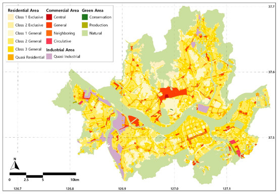
Figure 1.
Special-Purpose Area (SPA) of Seoul.
It is not practical to classify and analyze models based on 16 detailed SPAs; therefore, we reclassified the SPAs for the analysis. First, we excluded from the analysis of industrial areas and green areas where pedestrian patterns differ from general urban spaces. For the same reason, we also excluded circulative commercial areas for logistics facilities. The remaining SPAs can be largely divided into residential and commercial areas. However, because residential and commercial facilities are mixed in a quasi-residential area, we classified them as mixed-use areas. The reclassification is as follows: Residential, commercial, and mixed-use areas, as displayed on the right side of Table 1.
Figure 2 shows the monthly temperature changes in Seoul. The maximum temperature in Seoul during the year is 34.4 °C, and the minimum temperature is −12.9 °C, which is a difference of nearly 50 °C. In other words, the seasonal climate change is very large in Korea, which indicates that there is a limit to the analysis with a one-season model. Therefore, the models were classified according to seasons in this study.
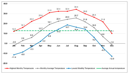
Figure 2.
Monthly temperature change in Seoul (2009).
It is ideal for building a model for each of Korea’s four seasons; however, there are limitations in the data that prevent this. This study used 2009 Pedestrian Volume Survey (PVS) data prepared by the Seoul Metropolitan Government (SMG). The SMG implemented PVS in 2009, 2012, 2013, 2014, and 2015 with the goal of establishing the world’s largest pedestrian volume database [46]. As shown in Table 2, the 2009 PVS had the most survey points, and was measured over the longest period. The 2009 PVS data only includes four months of data (from August to November), even though this survey covered a longer period of time than all existing PVSs. Therefore, there is a limit to creating a model that reflects the characteristics of all four seasons.
Table 2.
Survey points and survey periods of Pedestrian Volume Surveys (PVSs).
From August to November, October is the month in which the average monthly temperature is the closest to the annual average temperature (12.9 °C), and it is the most preferred month for cool and pleasant weather. Therefore, we extracted the October data, which was set as the base model. In addition, we extracted the August data, which was set as the hot weather model given that August has the highest temperatures. The average temperature in August is 25.7 °C, and the maximum temperature is 34.4 °C. Therefore, the influence of microclimate on PV in extremely hot climates can be analyzed using the August model. In addition, the average temperature in Korea is rising because of climate change, and the frequency of the occurrence of extremely hot weather is increasing [7]. Therefore, the hot weather model is expected to be helpful in estimating the change in the relationship between weather and walking in Korea in the future.
Through the above process, as shown in Table 3, we set eight models based on season and land-use. We divided the seasons into two categories: Autumn and summer, and we divided land-use into four categories: Total, residential, commercial, and mixed-use.
Table 3.
Classification of models.
2.2. Analysis Method
As shown in Figure 3, PV, the dependent variable, has large skewness and kurtosis and is skewed to the left. That is, the dependent variable is not normally distributed. In such cases, it is necessary to use a generalized linear model, since the widely used OLS regression model cannot be used. Among the generalized linear models, when the dependent variable is a countable variable, either a Poisson regression analysis or negative binomial regression analysis can be used [47]. We conducted a goodness-of-fit analysis, and subsequently, determined that a negative binomial regression analysis is most suitable for this data. A negative binomial regression is a statistical model used in various fields and has been proven to be highly effective in many existing studies in similar fields [24]. As mentioned previously, we used PV as the dependent variable and the microclimatic factors (temperature, precipitation, and PM10) as independent variables. Section 2.4 provides details on the configuration of the specific variables and the data construction methods.
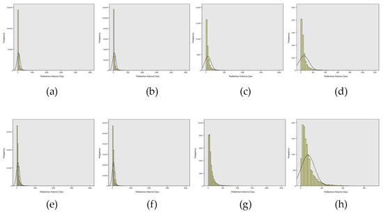
Figure 3.
Histogram of PV: (a) Model 1; (b) Model 2; (c) Model 3; (d) Model 4; (e) Model 5; (f) Model 6; (g) Model 7; (h) Model 8.
2.3. Data Source and Data Construction
As mentioned earlier, this study used 2009 PVS data provided by SMG because the 2009 PVS is the only dataset that can be analyzed for seasonal changes, as it includes survey data from August to November. Since the relationship between microclimatic factors and walking behavior is not expected to change significantly over time, the limitation of not using the latest data is not significant. Accordingly, the temporal scope of this study is 2009, and the spatial scope is the city of Seoul.
As explained above, we extracted the October and August data from the 2009 PVS dataset to build models. Therefore, out of the total PVS survey points, we only extracted the points that were surveyed in October and August. In addition, we extracted the points that were surveyed in three land-use areas (residential, commercial, and mixed-use). Accordingly, Figure 4 illustrates the PVS survey points included in this study. PVS points for August are marked with circles, and PVS points for October are marked with X. Table 4 shows the number of PVS survey points included in each model.
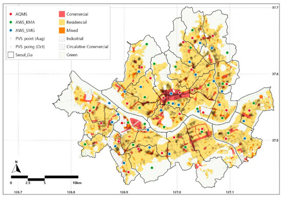
Figure 4.
PVS point, automatic weather station (AWS), and air quality monitoring station (AQMS) locations in Seoul.
Table 4.
The number of samples and survey points by model.
The PV survey is performed multiple times at one PVS point. Basically, five days of surveys are made according to the day of the week at one PVS point. The days of the week are divided into five categories: Monday, Tuesday/Thursday, Wednesday, Friday, and Saturday. At each PVS point, five days’ surveys must be done between August and November. Most points were surveyed for five days in the same month. However, there are some points in which the five days’ investigations were not completed in the same month because of the survey schedule. At points like these, investigations will continue next month. In addition, depending on the characteristics of the point, there are some points that are only surveyed on weekdays and only on weekends. In this study, only weekday data were used, excluding data on Saturdays where walking behavior is expected to be different. For this reason, the number of survey days per month appears from 1 to 4, depending on the point.
The daily survey was conducted from 7:30 to 21:30, and the survey was conducted by counting the number of pedestrians at the survey point. The investigator observes the number of pedestrians for five minutes, then records them and rests for 10 minutes. Therefore, data on the PV at each PVS point are generated every 15 minutes, and the value of PV in this data indicates the number of pedestrians counted for five minutes at each PVS point. This study attempted to construct data in as small a time unit as possible because microscopic microclimatic factor fluctuations affect the PV.
PVS data are provided in 15-minutes units, but microclimatic factor data are provided in 1-h units. Therefore, we summed the four units of PV values and set the value as the 1-h PV. The PV value derived in this way is the PV measured for 20 minutes, excluding the recording and resting time; therefore, it can be interpreted as 1/3 of the total PV for that period. The PV values summed in 1-h units were used as the dependent variable in this study. Table 4 shows the number of samples included in each model. The number of samples is much larger than the number of PVS points because surveys are conducted at one point over several days and times. Samples with missing values among the variables were excluded from the models.
It would be ideal if microclimatic data were measured for each PVS point; however, microclimatic data were not measured at many points. In Seoul, there are 25 air quality monitoring stations (AQMS) measuring PM10 data and 52 automatic weather stations (AWS) measuring weather data. All AQMS in Seoul are operated by the Korea Environment Corporation, while AWSs are operated by the Korea Meteorological Administration (KMA) and the SMG. In Figure 4, AWS operated by KMA are indicated by a green circle, and AWS operated by the SMG are indicated by a blue circle. AQMS collects SO2, CO, O3, NO2, and PM10 data [48], and AWS collects temperature, wind direction, wind speed, precipitation, humidity, and air pressure data [49]. We used the PM and weather values measured at the nearest AQMS and AWS at each PVS point as the PM and weather values for that PVS point. The locations of the AQMS and AWS are shown in Figure 4, and they are evenly distributed throughout Seoul.
2.4. Variables
Table 5 summarizes the variables used in this study. As described above, the dependent variable is PV constructed through PVS by the SMG. As microclimatic factor variables, temperature, precipitation, and particulate matter were included in the model as independent variables. The PM10 data measured by the nearest AQMS were used as the PM variable. PM10 is measured by the concentration of particles in the air of 10 μm or less. The weather variable was measured from the nearest AWS. The AWS measures temperature, precipitation, wind speed, wind direction, air pressure, and humidity. Among these weather variables, we included temperature and precipitation in the model. This is because temperature and precipitation are known to affect walking and have the same values in a relatively large area. Wind direction and wind speed change greatly depending on the location. Therefore, it is difficult to assume that the value measured in the nearest AWS is the value of the PVS point.
Table 5.
List of variables included in this study.
The physical environment of the city has a great influence on PV. In Korea, it is known that land-use-related variables [50,51] and micro-environmental factors affect PV [13,52,53]. In this study, since the model was classified by land-use, variables related to land-use were not included in the models. There is a limit to establishing microscopic environmental variables of more than 3000 PVS points. Accordingly, we included the number of lanes and bus stops in the model as variables representing the microscopic environmental factors of the street. The number of lanes can represent the hierarchy and width of the street, and bus stops can represent accessibility to public transport. The bus stop variable was constructed in the form of a dummy variable that measures whether or not there is a bus stop within 50m from each PVS point.
Since the PVS was surveyed from 7:30 to 21:30, there are 14 time periods in 1-h unit PV data. The time period is also known to have a great influence on the PV in urban spaces [53,54]. Therefore, it is necessary to control the change in PV according to the time period. For this purpose, 14 time periods were divided into six time periods according to their characteristics and included in the model in the form of nominal variables.
3. Results
3.1. Descriptive Statistics
Table 6 summarizes the descriptive statistics of the ratio scale variables included in each model, and Table 7 summarizes the descriptive statistics of the nominal scale variables. As for the dependent variable, the average value of PV is 58.94 in the total land-use model in autumn (Model 1) and 65.49 in the total land-use model in summer (Model 5). In regard to the land-use area, the average PV of residential areas (60.66) is highest in autumn, but the average PV of the commercial areas (96.17) is highest in summer.
Table 6.
Descriptive statistics for the ratio scale variables.
Table 7.
Descriptive statistics for the nominal scale variables.
As explained above, the difference in climate by season in Korea is quite large. The average temperature of Model 1 (autumn) was 17.69, and the average temperature of Model 5 (summer) was 27.66. The mean value of precipitation in Model 1 was 0.60, and the mean value in Model 5 was 4.64. The maximum value of precipitation is 19.5 for Model 1 and 114 for Model 5, which is even greater. This is because torrential rains occur mainly in summer in Korea. The average PM10 value of Model 1 is 53.73, which is higher than the WHO daily average guideline of 50 µg/m³ [55]. The average PM10 value of Model 5 is 32.02, which is much smaller than that of Model 1. However, the maximum PM10 value is 180 in Model 1 and 170 in Model 5, and the difference is not significant.
The average value for each model for a number of lanes, which is a control variable, represents a value between 2.5 and 3.5. The PVS survey was mainly conducted on streets with between two and four lanes. In regard to the time period variable, “afternoon” (which includes 4 hours) accounts for the most samples. Of the total sample, cases where there is a bus stop around the PVS point account for 20–30%.
3.2. Seasonal Differences in the Influence of Microclimate (Weather and Air Quality) on PV
Table 8 shows the results of the negative binomial regression analysis of Model 1 (autumn) and Model 5 (summer), including all land-use areas (residential, commercial, and mixed-use). The statistical significance level was set at 5%. According to Model 1, all microclimatic factor variables (temperature, precipitation, and PM10) have a statistically significant effect on PV. The temperature has a positive effect on PV, which means that PV increases as it gets warmer. Precipitation has a negative effect on PV, which means that PV decreases with more rain. PM10 has a negative effect on PV, which means that PV decreases as the concentration of PM increases.
Table 8.
Negative binominal regression analysis results by season.
According to the results of Model 5, unlike Model 1, temperature negatively affects PV, and PM10 does not have a significant effect. Precipitation has a significant negative effect on PV, as in Model 1. However, the coefficient value is −0.00185, which is only half of the value in Model 1 (−0.00349). The fact that the influence of independent variables, the direction of influence, and the magnitude of the influence differ depending on the season indicates that there is a large difference in the effect of microclimatic factors on PV by season. In addition, it confirms the necessity of analyzing this topic with models that have been classified by season.
Most time periods have the effect of increasing PV compared to the reference item (early morning). The number of lanes has a significant positive effect on PV in both models. However, the coefficient value in Model 1 is 0.01450, which is 1/5 of the value (0.07695) in Model 5. This means that in autumn, pedestrians are less crowded in large streets than in summer. Autumn is the season with the most pleasant weather, and many pedestrians are crowded on small roads and alleys rather than large streets. Such results were also observed in a previous study [56]. In addition, the bus stop variable has no significant effect in Model 1. In other words, the phenomenon where pedestrians gather on the main street near bus stops does not occur in autumn.
3.3. Difference in Influences of Microclimate (Weather and Air Quality) on PV by Land-Use
Table 9 shows the results of the negative binomial regression analyses for Models 2, 3, and 4, which classified autumn data by land-use. The statistical significance level was set at 5%. As shown in Table 9, there is a difference in the influence of microclimatic factors on PV depending on the land-use area. First, in residential areas (Model 2), the microclimatic factor variables had a significant effect on PV. The higher the temperature, the less precipitation, and the lower the PM10, the higher the PV. On the other hand, in commercial areas (Model 3), only precipitation had a significant effect on PV, while temperature and PM10 did not affect PV. In mixed-use areas (Model 4), where residential and commercial uses were mixed, temperature and precipitation had a significant effect on PV. The temperature has a positive effect, and precipitation has a negative effect. Because the uses of residential and commercial areas are mixed, the effects of microclimate also have an intermediate character between residential and commercial areas.
Table 9.
Negative binominal regression analysis results by land-use (autumn).
The coefficient of precipitation, which represents a significant effect on all three land-use areas, indicates that the residential area is −0.00226, the mixed-use area is −0.00924, and the commercial area is −0.00970. That is, the magnitude of the influence of precipitation on PV is the largest in commercial areas and the smallest in residential areas, with the mixed-use areas falling in the middle. In other words, the number of microclimatic factor variables that have a significant influence on PV is the largest in residential areas, but the influence of variables that have a significant effect on the PV increases as the proportion of commercial functions increases.
Among the control variables, time periods showed similar results to total land-use (Model 1). The number of lanes had a significant positive effect on PV in residential and mixed-use areas. On the other hand, there was no significant effect on the commercial area. It is believed that this is because wide roads in commercial areas are often not comfortable for walking because of noise and exhaust gas. It is likely that this also explains why bus stops exhibit a negative effect on PV in commercial and mixed-use areas.
Table 10 shows the results of Models 6, 7, and 8, which classified summer data by land-use. In residential areas (Model 6), all microclimatic variables had a significant effect on PV. In particular, PM, which did not affect the total land-use model (Model 5), also affected PV. In the commercial area (Model 6), none of the microclimate variables significantly affected PV. In particular, precipitation, which had an effect in commercial areas in autumn (Model 3), did not have a significant effect. In mixed-use areas, temperature and PM10 have a significant negative effect, and the magnitude of the effect is very large compared to residential areas. Similar to the autumn models, it is thought that the influence of microclimatic factor variables increases when commercial functions are mixed.
Table 10.
Negative binominal regression analysis results by land-use (summer).
The control variables show similar results to the summer total model (Model 5). The number of bus stops and lanes has a significant positive effect on PV. Unlike au-tumn, it is thought that pedestrians prefer wide streets in summer.
4. Discussion
For a compact discussion, Table 11 summarizes only the coefficients of the microclimatic variables in the eight negative binomial regression models. Based on the significance level of 5%, only the coefficient values of variables that have a significant effect on PV are indicated, and variables without significant effect are indicated as blanks. According to the results, the influence of microclimatic factors on PV is clearly different according to land-use, and seasonal differences also appear.
Table 11.
Summary of the microclimatic variable regression coefficients.
Comparing Model 1 and Model 5, we can see a distinct seasonal difference. First, in autumn and summer, the influence of temperature variables is reversed. In autumn, it has a positive effect (0.00513), while it has a negative effect in summer (−0.00545). This is because summer in Korea is very hot. In many studies, the temperature has a positive effect on outdoor activities [31], but studies in Texas (with its hot climate) have shown negative effects [32]. Another difference in the comparison between Model 1 and Model 5 is that PM10 has a significant effect only in Model 1. This is likely because the average PM concentration in summer is lower than in autumn. As shown in Table 6, the average of PM10 in summer (Model 5) is 32.02, which is lower than that of 53.73 in autumn (Model 1). In addition, 32.02 is lower than the WHO’s daily average PM10 guideline of 50 µg/m³ [55].
The analysis results of the models divided by land-use identified a number of notable features, which are as follows. First, there are more microclimatic factors affecting PV in residential areas than in commercial areas. In residential area models (Models 2 and 6), all three microclimatic variables had significant effects on PV, whereas, among commercial area models (Models 3 and 7), only the precipitation variables in Model 3 showed significant effects. This is thought to be due to the large number of people in residential areas that are sensitive to weather and air pollution, such as children and the elderly. Such a sensitive class seems to adjust the amount of walking in response to various microclimatic factors. Particularly, PM10, which did not have a significant effect on the total land-use model in summer (Model 5), has a significant effect in the residential area model in summer (Model 6). As stated above, the overall PM concentration in summer is lower than in autumn. Nevertheless, pedestrians in residential areas are sensitive to this.
Second, the size of the influence of the microclimatic variables in commercial or mixed-use areas is greater than that of residential areas. In other words, in areas with more commercial functions than residential functions, the size of the influence of the microclimatic variables increases. When observing the absolute values of the coefficients in the autumn models, the coefficient of precipitation is large in the order of commercial (−0.00970), mixed-use (−0.00924), and residential (−0.00465). The coefficient of temperature is also twice as high in mixed-use areas (0.01327) compared to residential areas (0.00602). Among the summer models, commercial areas do not have significant microclimatic variables, so mixed-use areas and residential areas can be compared. In the mixed-use area (Model 8), the coefficient of temperature is −0.01019, and the coefficient of PM10 is −0.00119. This is very large compared to the absolute value of the coefficient (temperature −0.00524, PM10 −0.00039) in residential areas (Model 6). This is thought to be because there are various options for transportation in commercial areas, compared to residential areas. Therefore, it is thought that the decrease in PV due to bad weather or air pollution is greater than in residential areas.
Third, the influence of microclimatic factors on PV in mixed-use areas has intermediate characteristics between residential and commercial areas. The number of microclimate variables that have a significant effect on PV in mixed-use areas is the value between residential and commercial areas. The coefficient value of the significant variable also represents the value between residential and commercial areas. This suggests that changes in building use and density according to land-use can induce a gradual change in the influence of microclimatic factors on PV.
Fourth, the influence of temperature and precipitation on PV has seasonality. The direction of the influence of temperature on PV in the summer models is opposite to that of the autumn models. Precipitation had a significant effect on PV in all land-uses in autumn, but only in residential areas in summer. This result is because the level of climate elements in Korea varies greatly from season to season, as shown in Figure 2 and Table 6. Considering this seasonality, when data becomes available, follow-up studies through winter and spring models are needed.
5. Conclusions
This study analyzed whether the influence of microclimatic factors on PV differs according to land-use. Eight models classified according to season and land-use were analyzed using negative binomial regression analysis, and it was confirmed that the influence of microclimate factors on PV differs according to land-use. In residential areas, all microclimate variables affected PV, but only a very limited number of variables affected PV in commercial areas. On the other hand, the size of the influence of the significant microclimatic variables was larger in the commercial areas, or the areas where commercial functions were mixed, than in the residential areas. In addition, in the mixed-use areas, the influence of microclimate factors on PV was intermediate between residential and commercial areas.
The results of this study suggest several implications for urban planning. First, efforts to solve the problem of reduced PV caused by bad microclimatic conditions must be different for each land-use. Reducing PV reduces the vitality of cities, and many city governments are trying to mitigate the negative effects of microclimate. According to the results of this study, a differentiated policy for each land-use is required because the influence of microclimatic factors on PV is very different for each land-use. Second, it is possible to offset the negative effects of microclimatic factors on PV through the mixing of land-uses. According to the results of this study, the influence of microclimatic factors in the mixed-use area showed intermediate characteristics between residential and commercial areas. Therefore, it is expected to be able to offset weaknesses from the influence of microclimatic factors in each land-use area through the mixing of land-uses.
This study makes the following contributions: This is an early study that demonstrated that the effects of microclimate on PV may vary depending on land-use. In particular, in addition to the general weather factors, the inclusion of PM, which is a problem in many cities, can be suggested as the significance of the study. In addition, this study compared autumn (the season with the general climate of Korea) with the very hot season. Through this, it is possible to predict the change in the direction of PV in the future due to climate change.
However, this study has some limitations. It is possible that the 2009 data do not reflect the latest pedestrian behavior, though we think this is unlikely. In addition, the generalization of the results may be limited by using data from one city. Another limitation of the PV data used in this study is that there is no trip purpose information. Therefore, there is a limitation in the interpretation of research results based on the trip purpose. These challenges are due to the limitations of the data. If more data are provided in the future, it will be possible to conduct research that overcomes these limitations. Moreover, this study’s design did not reflect the more diversely classified land-uses. Therefore, there is a need for a study that clarifies the difference in the influence of microclimatic factors on PV based on more detailed land-use.
Author Contributions
Conceptualization, H.K. and S.H.; methodology, S.H.; data curation, S.H.; writing—original draft preparation, H.K. and S.H.; writing—review and editing, H.K. and S.H. All authors have read and agreed to the published version of the manuscript.
Funding
This research received no external funding.
Institutional Review Board Statement
The study was conducted according to the guidelines of the Declaration of Helsinki, and approved by the Institutional Review Board of Chungbuk National University (CBNU-202004-ETC-0039, 10 April 2020).
Conflicts of Interest
The authors declare no conflict of interest.
References
- Whyte, W. The Social Life of Small Urban Spaces; The Conservation Foundation: New York, NY, USA, 1980; ISBN 0-89164-057-6. [Google Scholar]
- Lynch, K. Good City Form; Reprint edition; The MIT Press: Cambridge, MA, USA, 1984; ISBN 978-0-262-62046-8. [Google Scholar]
- Lenzholzer, S.; Van der Wulp, N. Thermal Experience and Perception of the Built Environment in Dutch Urban Squares. J. Urban Des. 2010, 15, 375–401. [Google Scholar] [CrossRef]
- Norton, B.A.; Coutts, A.M.; Livesley, S.J.; Harris, R.J.; Hunter, A.M.; Williams, N.S.G. Planning for cooler cities: A framework to prioritise green infrastructure to mitigate high temperatures in urban landscapes. Landsc. Urban Plan. 2015, 134, 127–138. [Google Scholar] [CrossRef]
- Whitman, S.; Good, G.; Donoghue, E.R.; Benbow, N.; Shou, W.; Mou, S. Mortality in Chicago attributed to the July 1995 heat wave. Am. J. Public Health 1997, 87, 1515–1518. [Google Scholar] [CrossRef]
- Dhainaut, J.-F.; Claessens, Y.-E.; Ginsburg, C.; Riou, B. Unprecedented heat-related deaths during the 2003 heat wave in Paris: Consequences on emergency departments. Crit. Care 2004, 8, 1–2. [Google Scholar] [CrossRef]
- Government of Korea. 2019 Abnormal Climate Report; Korea Meteorological Administration: Seoul, Korea, 2019.
- Kwon, M.Y.; Lee, J.S.; Park, S. The effect of outdoor air pollutants and greenness on allergic rhinitis incidence rates: A cross-sectional study in Seoul, Korea. Int. J. Sustain. Dev. World Ecol. 2019, 26, 258–267. [Google Scholar] [CrossRef]
- World Health Organization Ambient (Outdoor) Air Pollution. Available online: https://www.who.int/news-room/fact-sheets/detail/ambient-(outdoor)-air-quality-and-health (accessed on 8 August 2020).
- OECD. The Economic Consequences of Outdoor Air Pollution; OECD Publishing: Paris, France, 2016; ISBN 978-92-64-25747-4. [Google Scholar]
- Jacobs, J. The Death and Life of Great American Cities; Random House: New York, NY, USA, 1961; ISBN 978-0-394-42159-9. [Google Scholar]
- Ewing, R.; Cervero, R. Travel and the Built Environment. J. Am. Plann. Assoc. 2010, 76, 265–294. [Google Scholar] [CrossRef]
- Kim, H.; Ahn, K.-H.; Kwon, Y.-S. The Effects of Residential Environmental Factors on Personal Walking Probability—Focused on Seoul. J. Urban Des. Inst. Korea 2014, 15, 5–18. [Google Scholar]
- Perry, J. Climate change adaptation in the world’s best places: A wicked problem in need of immediate attention. Landsc. Urban Plan. 2015, 133, 1–11. [Google Scholar] [CrossRef]
- Gehl, J.; Svarre, B. How to Study Public Life; Illustrated edition; Island Press: Washington, DC, USA, 2013; ISBN 978-1-61091-423-9. [Google Scholar]
- Frank, L.D.; Sallis, J.F.; Conway, T.L.; Chapman, J.E.; Saelens, B.E.; Bachman, W. Many Pathways from Land Use to Health: Associations between Neighborhood Walkability and Active Transportation, Body Mass Index, and Air Quality. J. Am. Plan. Assoc. 2006, 72, 75–87. [Google Scholar] [CrossRef]
- Frank, L.D.; Engelke, P. Multiple Impacts of the Built Environment on Public Health: Walkable Places and the Exposure to Air Pollution. Int. Reg. Sci. Rev. 2005, 28, 193–216. [Google Scholar] [CrossRef]
- Cervero, R.; Kockelman, K. Travel demand and the 3Ds: Density, diversity, and design. Transp. Res. Part Transp. Environ. 1997, 2, 199–219. [Google Scholar] [CrossRef]
- Ewing, R.; Bartholomew, K.; Winkelman, S.; Walters, J.; Chen, D. Growing Cooler: Evidence on Urban Development and Climate Change; Urban Land Institute: Chicago, IL, USA, 2007; ISBN 978-0-87420-082-9. [Google Scholar]
- Ahn, S.-E.; Bae, H.-J.; Kwak, S.-Y.; Im, Y.-H.; Kim, M.-H.; Oh, S.-Y. Assessment of Human Health Effects of Air-Pollution Using Cohort DB and Estimation of Associated Economic Costs in Korea (II); Korea Environment Institute: Sejong, Korea, 2016; ISBN 979-11-5980-091-7.
- Brook, R.D.; Rajagopalan, S.; Pope, C.A.; Brook, J.R.; Bhatnagar, A.; Diez-Roux, A.V.; Holguin, F.; Hong, Y.; Luepker, R.V.; Mittleman, M.A.; et al. Particulate matter air pollution and cardiovascular disease: An update to the scientific statement from the American Heart Association. Circulation 2010, 121, 2331–2378. [Google Scholar] [CrossRef]
- Dockery, D.W.; Pope, C.A.; Xu, X.; Spengler, J.D.; Ware, J.H.; Fay, M.E.; Ferris, B.G.; Speizer, F.E. An Association between Air Pollution and Mortality in Six U.S. Cities. N. Engl. J. Med. 1993, 329, 1753–1759. [Google Scholar] [CrossRef]
- Kim, H. Land Use Impacts on Particulate Matter Levels in Seoul, South Korea: Comparing High and Low Seasons. Land 2020, 9, 142. [Google Scholar] [CrossRef]
- Kim, H. Seasonal Impacts of Particulate Matter Levels on Bike Sharing in Seoul, South Korea. Int. J. Environ. Res. Public Health 2020, 17, 3999. [Google Scholar] [CrossRef]
- Carmona, M.; Tiesdell, S. Urban Design Reader; Routledge: London, UK, 2007; ISBN 978-0-7506-6531-5. [Google Scholar]
- Carr, S.; Francis, M.; Rivlin, L.G.; Stone, A.M. Public Space; Cambridge University Press: Cambridge, UK, 2009; ISBN 978-0-521-35148-5. [Google Scholar]
- Gehl, J. Life between Buildings: Using Public Space, 6th ed.; Island Press: Washington, DC, USA, 2011; ISBN 978-1-59726-827-1. [Google Scholar]
- Perini, K.; Magliocco, A. Effects of vegetation, urban density, building height, and atmospheric conditions on local temperatures and thermal comfort. Urban For. Urban Green. 2014, 13, 495–506. [Google Scholar] [CrossRef]
- Klemm, W.; Heusinkveld, B.G.; Lenzholzer, S.; van Hove, B. Street greenery and its physical and psychological impact on thermal comfort. Landsc. Urban Plan. 2015, 138, 87–98. [Google Scholar] [CrossRef]
- Humpel, N.; Owen, N.; Iverson, D.; Leslie, E.; Bauman, A. Perceived environment attributes, residential location, and walking for particular purposes. Am. J. Prev. Med. 2004, 26, 119–125. [Google Scholar] [CrossRef]
- Tucker, P.; Gilliland, J. The Effect of Season and Weather on Physical Activity: A Systematic Review. Public Health 2007, 121, 909–922. [Google Scholar] [CrossRef]
- Baranowski, T.; Thompson, W.O.; Durant, R.H.; Baranowski, J.; Puhl, J. Observations on Physical Activity in Physical Locations: Ager Gender, Ethnicity, and Month Effects. Res. Q. Exerc. Sport 1993, 64, 127–133. [Google Scholar] [CrossRef]
- Bitar, A.; Fellmann, N.; Vernet, J.; Coudert, J.; Vermorel, M. Variations and determinants of energy expenditure as measured by whole-body calorimetry during puberty and adolescence. Am. J. Clin. Nutr. 1999, 69, 1209–1216. [Google Scholar] [CrossRef]
- Levin, S.; Jacobs, D.R.; Ainsworth, B.E.; Richardson, M.T.; Leon, A.S. Intra-Individual Variation and Estimates of Usual Physical Activity. Ann. Epidemiol. 1999, 9, 481–488. [Google Scholar] [CrossRef]
- Gordon-Larsen, P.; Mcmurray, R.; Popkin, B. Determinants of adolescent physical activity and inactivity patterns. Pediatrics 2000, 105, e83. [Google Scholar] [CrossRef]
- Pivarnik, J.M.; Reeves, M.J.; Rafferty, A.P. Seasonal variation in adult leisure-time physical activity. Med. Sci. Sports Exerc. 2003, 35, 1004–1008. [Google Scholar] [CrossRef]
- Plasqui, G.; Westerterp, K. Seasonal Variation in Total Energy Expenditure and Physical Activity in Dutch Young Adults. Obes. Res. 2004, 12, 688–694. [Google Scholar] [CrossRef]
- Schweitzer, L.; Zhou, J. Neighborhood Air Quality, Respiratory Health, and Vulnerable Populations in Compact and Sprawled Regions. J. Am. Plann. Assoc. 2010, 76, 363–371. [Google Scholar] [CrossRef]
- Yan, L.; Duarte, F.; Wang, D.; Zheng, S.; Ratti, C. Exploring the effect of air pollution on social activity in China using geotagged social media check-in data. Cities 2019, 91, 116–125. [Google Scholar] [CrossRef]
- Bresnahan, B.W.; Dickie, M.; Gerking, S. Averting Behavior and Urban Air Pollution. Land Econ. 1997, 73, 340–357. [Google Scholar] [CrossRef]
- Neidell, M. Information, Avoidance Behavior, and Health. J. Hum. Resour. 2009, 44, 450–478. [Google Scholar] [CrossRef]
- Chung, J.; Kim, S.-N.; Kim, H. The Impact of PM10 Levels on Pedestrian Volume: Findings from Streets in Seoul, South Korea. Int. J. Environ. Res. Public. Health 2019, 16, 4833. [Google Scholar] [CrossRef]
- Lee, H.; Kim, N. The Impact of Fine Particular Matter Risk Perception on the Outdoor Behavior of Recreationists: An Application of the Extended Theory of Planned Behavior. J. Tour. Sci. 2017, 41, 27–44. [Google Scholar]
- Yoon, H. Effects of particulate matter (PM10) on tourism sales revenue: A generalized additive modeling approach. Tour. Manag. 2019, 74, 358–369. [Google Scholar] [CrossRef]
- National Land Planning and Utilization Act of 2019, Article 36. Available online: https://elaw.klri.re.kr/eng_mobile/viewer.do?hseq=25486&type=sogan&key=4 (accessed on 4 February 2020).
- Seoul Metropolitan Government; National Information Society Agency. 2015 Seoul Pedestrian Volume Survey Report; Seoul Metropolitan Government: Seoul, Korea, 2015; p. 81.
- Lee, I.-H. Easy Flow Regression Analysis; Hannarae Publishing: Seoul, Korea, 2014; ISBN 978-89-5566-155-2. [Google Scholar]
- Air Quality Data. Available online: https://www.airkorea.or.kr/web/autoStatistic?pMENU_NO=123 (accessed on 22 December 2020).
- AWS Weather Data. Available online: https://data.kma.go.kr/data/grnd/selectAwsRltmList.do?pgmNo=56 (accessed on 22 December 2020).
- Im, H.N.; Lee, S.; Choi, C. Empirical Analysis of the Relationship between Land Use Mix and Pedestrian Volume in Seoul, Korea. J. Korea Plan. Assoc. 2016, 51, 21. [Google Scholar] [CrossRef]
- Jang, J.-Y.; Choi, S.-T.; Lee, H.-S.; Kim, S.-J.; Choo, S.-H. A comparison analysis of factors to affect pedestrian volumes by land-use type using Seoul Pedestrian Survey data. J. Korea Inst. Intell. Transp. Syst. 2015, 14, 39–53. [Google Scholar] [CrossRef]
- Hong, S.; Lee, K.-H.; Ahn, K.-H. The Effect of Street Environment on Pedestrians’ Purchase in Commercial Street—Focused on Insa-dong and Munjeong-dong Commercial Street. J. Archit. Inst. Korea Plan. Des. 2010, 26, 229–237. [Google Scholar]
- Lee, J.; Kim, H.; Jun, C. Analysis of Physical Environmental Factors that Affect Pedestrian Volumes by Street Type. J. Urban Des. Inst. Korea 2015, 16, 123–141. [Google Scholar]
- Lee, G. The Effect of the Urban and Architectural Form Factors on Pedestrian Volume. J. Korea Acad. Ind. Coop. Soc. 2016, 17, 310–318. [Google Scholar] [CrossRef]
- World Health Organization. WHO Air Quality Guidelines for Particulate Matter, Ozone, Nitrogen Dioxide and Sulfur Dioxide—Global Update 2005; World Health Organization: Geneva, Switzerland, 2006. [Google Scholar]
- Lee, S.; Hong, S. The Effect of Weather and Season on Pedestrian Volume in Urban Space. J. Korea Acad. Ind. Coop. Soc. 2019, 20, 56–65. [Google Scholar] [CrossRef]
Publisher’s Note: MDPI stays neutral with regard to jurisdictional claims in published maps and institutional affiliations. |
© 2021 by the authors. Licensee MDPI, Basel, Switzerland. This article is an open access article distributed under the terms and conditions of the Creative Commons Attribution (CC BY) license (http://creativecommons.org/licenses/by/4.0/).