Multilayer Substrate Configuration Enhances Removal Efficiency of Pollutants in Constructed Wetlands

Abstract

This study aimed at optimizing horizontal subsurface flow constructed wetlands (CWs) to improve hydraulic performance and pollutant removal efficiency. A groundwater modeling package (MODFLOW) was used to optimize three design parameters (length-to-width ratio, inlet/outlet-to-length ratio, and substrate size configuration). Using the optimized parameters, three pilot-scale CWs were built to treat actual wastewater. For model validation, we used a tracer test to evaluate hydraulic performance, and investigated the pollutant spatial distributions and removal efficiencies. We conclude that MODFLOW is suitable for designing CWs, accurately predicting that increasing hydraulic conductivity from surface to bottom layers could improve performance. However, the effect of vegetation, which decreased the hydraulic conductivity of the surface layer, should be considered to improve simulation results. Multilayer substrate configuration, with increasing hydraulic conductivity from the surface to bottom layers, significantly increased pollutant removal compared with monolayer configuration. The spatial variation in pollutant transport and degradation through the filling substrate showed that the multilayer configuration was able to increase use of the available space and moderately reduced short-circuiting and dead zones. Thus, multilayer CWs had higher experimental retention times, effective volume fractions and hydraulic efficiencies, and lower short-circuiting compared with monolayer CWs operating under similar conditions.

1. Introduction

As an economic, robust, and sustainable technology, horizontal subsurface flow constructed wetlands (hereafter simplified to CWs) have been widely used for the treatment of domestic, agricultural, and industrial wastewater [1,2]. In an ideally designed CW, water should flow horizontally from the inlet through the wetland bed to the outlet, with very little hydraulic dispersion. However, poor hydrodynamic behavior due to clogging is commonly found in full-scale CWs and have resulted in preferential flow pathways and dead zones [3]. Clogging may cause a large proportion of the water to pass over the bed as surface runoff, thus significantly reducing the effective volume of the system for removing waste [4]. The resulting ineffective wetland bed leads to incomplete biodegradation and reduces the performance of CWs [5,6].

In recent years, CW design has evolved to mitigate the adverse effects of clogging [4,7]. Previous studies aimed at increasing hydraulic retention time and maximizing contact opportunity between the substrate and wastewater to improve treatment performance [8]. Some important design parameters affecting retention time in CWs include length-to-width ratio, inlet/outlet-to-length ratio, and configuration of substrate size. According to García, et al. [9], the length-to-width ratio is one of the most important factors for enhancing the hydraulic and treatment performance of CWs. A relatively high length-to-width ratio can improve hydraulic behavior by reducing the internal dispersion of the water flow, thus forcing the water to pass through the whole cross-section of the wetland bed [10]. In recent years, the design of CWs with a low length-to-width ratio (<1) and large inlet cross-section was also designed to reduce the impact of total suspended solids (TSS) on the clogging in the first part of CWs’ bed. However, spreading the influent over too wide an area presents a number of hydraulic challenges, especially for small systems, where the flow rate is close to zero [11]. The inlet/outlet-to-length ratio—defined as the ratio of the length of the inlet distribution zone or the outlet collection zone to the whole length of the CW—is also important to prevent the development of preferential paths and dead zones and, thus, affects treatment efficiency [12]. The substrate used in CWs is also an important factor affecting pollutant removal because most pollutants are removed through biodegradation by biofilm. Substrate configuration can be improved by placing finer media with low hydraulic conductivity on the top and coarse media with high hydraulic conductivity on the bottom, which should theoretically prevent water short-circuiting of the water flow by passing on the surface and decreasing the dead zones at the bottom. It would also make the water flow pattern more uniform. Here, we must note that previous studies have predominantly been based on random selection of parameters [7]. No studies have accurately quantified water flow distribution by integrating different design parameters in CWs to improve hydraulic and treatment performance.

The aims of the present study are to optimize the hydraulic performance of CWs through a computer model simulation and to validate the model by measuring the hydraulic performance and pollutant removal efficiencies of pilot-scale systems that were built to model specifications (Figure 1). The computer simulation study was conducted using the MODFLOW modeling package, which is a finite difference block-centered three-dimensional groundwater modeling package. The modeling package can simulate steady-state and transient groundwater flows for different hydrogeological systems. Based on the characteristics, the modeling package may be suitable for quantifying the flow patterns in CWs [13,14]. To optimize the flow distribution, we manipulated three main design parameters: length-to-width ratio, inlet/outlet-to-length ratios, and configuration of substrate size. The crucial determining factor for the flow uniformity was identified from the simulation results. Subsequently, additional models were built to optimize the original models, mainly aiming to select the best values for the determining factors. Based on the optimized model parameters, three pilot-scale CWs were established to treat actual domestic wastewater and validate the model by measuring the hydraulic performance, spatial distribution of the pollutants and removal efficiency.

2. Materials and Methods

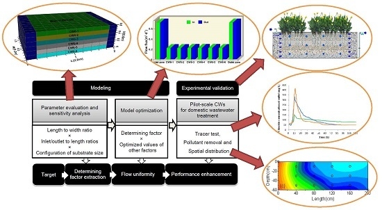
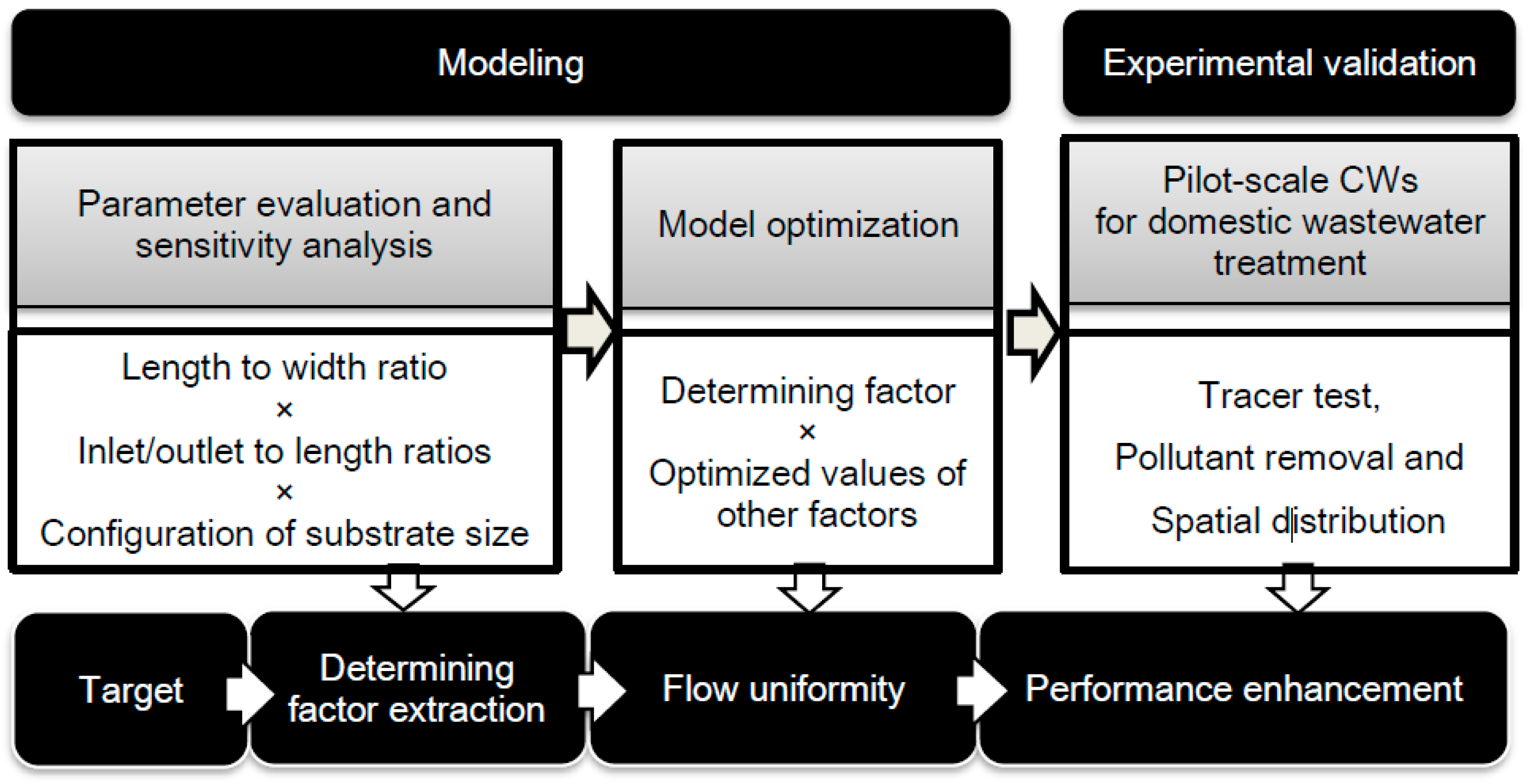
2.1. Modeling

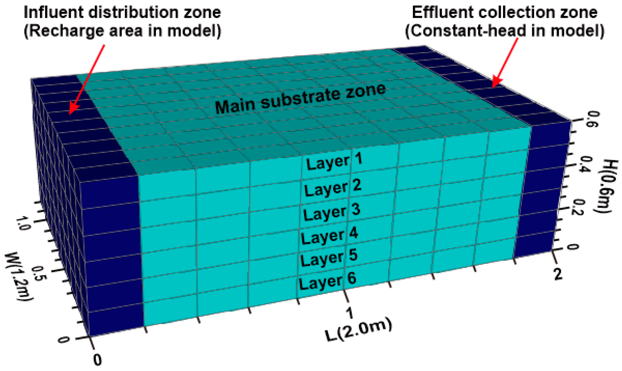
2.1.1. Model Domain Setup and Calculation

The software program Visual Modflow 4.0 (Waterloo Hydrogeologic, Kitchener, ON, Canada) was used to simulate the flow distributions in the CWs. A CW model domain was set that comprised an influent distribution zone, main substrate zone containing six equally spaced layers, and an effluent collection zone (Figure 2). The six layers can be combined or used separately. A regular grid of 10 × 10 cells was used throughout the model domain. A recharge boundary condition of 0.72 m³/day was assigned to the distribution zone of CWs using the Visual Modflow Recharge package. A common wetland depth of 0.6 m was chosen for all the modeling. Also, a constant head boundary condition (0.6 m) was assigned to the effluent collection zone. The length of the inlet zone (influent distribution zone) and outlet zone (effluent collection zone) were assigned equal values. The hydraulic conductivity (K value) of the substrate in the influent distribution and effluent collection zones was always set to 500 m/day. The K values of the substrate in the main substrate zone were varied according to configuration of substrate size during the model simulation.

The flow distributions in the CW model were calculated according to Equation (1) [15]:

$$\frac{\partial }{\partial x}\left(k_{xx}\frac{\partial h}{\partial x}\right)+\frac{\partial }{\partial y}\left(k_{yy}\frac{\partial h}{\partial y}\right)+\frac{\partial }{\partial z}\left(k_{zz}\frac{\partial h}{\partial z}\right)-w=S\frac{\partial h}{\partial t}$$

(1)

where $k_{xx},k_{yy},k_{zz}$ are the hydraulic conductivities along the x (width), y (length), and z (depth) coordinate axes, which are assumed to be parallel to the major axes of hydraulic conductivity (m/day); h is the potentiometric head (m); w is a volumetric flux per unit volume (m³/day water/m³ substrate; day⁻¹) representing sources and/or sinks of water, with w < 0 for flow out of the CW system and w > 0 for flow into the system; S is the specific storage of the porous material (m³ water/m³ substrate/m hydraulic head; m⁻¹); and t is time (day).

2.1.2. Model Evaluation

The simulations were conducted for the CW models using three length-to-width ratios (1:1, 2:1, and 3:1). Each model was assigned one of the three inlet/outlet-to-length ratios (1:5, 1:10, and 1:20). Additionally, for each combination of length-to-width ratio and inlet/outlet-to-length ratio, three configurations of substrate size and layout were used: (1) a monolayer configuration (substrate with K value of 200 m/day); (2) an ascending three-layer configuration (equally thick substrate layers with K values of 50, 100, and 200 m/day, respectively from surface to bottom); and (3) a descending three-layer configuration (equally thick substrates with K values of 200, 100, and 50 m/day, respectively from surface to bottom). The combination of three different length-to-width ratios, inlet/outlet-to-length ratios, and configurations of substrate size resulted in a complete model design with a series of 27 test models (

Table A1. Modeling test series with the parameters of length-to-width ratios, inlet/outlet-to-length ratios, and three configurations of the substrate size.

Models	Length to Width Ratios	Inlet/Outlet to Length Ratios	Configurations of Substrate Size, K (m/Day) (Listed in Order of Surface to Bottom Layers)
Model 1	1:1	1:5	monolayer, K = 200
Model 2	1:1	1:5	three-layers, K = 50, 100 and 200
Model 3	1:1	1:5	three-layers, K = 200, 100 and 50
Model 4	1:1	1:10	monolayer, K = 200
Model 5	1:1	1:10	three-layers, K = 50, 100 and 200
Model 6	1:1	1:10	three-layers, K = 200, 100 and 50
Model 7	1:1	1:20	monolayer, K = 200
Model 8	1:1	1:20	three-layers, K = 50, 100 and 200
Model 9	1:1	1:20	three-layers, K = 200, 100 and 50
Model 10	2:1	1:5	monolayer, K = 200
Model 11	2:1	1:5	three-layers, K = 50, 100 and 200
Model 12	2:1	1:5	three-layers, K = 200, 100 and 50
Model 13	2:1	1:10	monolayer, K = 200
Model 14	2:1	1:10	three-layers, K = 50, 100 and 200
Model 15	2:1	1:10	three-layers, K = 200, 100 and 50
Model 16	2:1	1:20	monolayers, K = 200
Model 17	2:1	1:20	three-layers, K = 50, 100 and 200
Model 18	2:1	1:20	three-layers, K = 200, 100 and 50
Model 19	3:1	1:5	monolayer, K = 200
Model 20	3:1	1:5	three-layers, K = 50, 100 and 200
Model 21	3:1	1:5	three-layers, K = 200, 100 and 50
Model 22	3:1	1:10	monolayer, K = 200
Model 23	3:1	1:10	three-layers, K = 50, 100 and 200
Model 24	3:1	1:10	three-layers, K = 200, 100 and 50
Model 25	3:1	1:20	monolayer, K = 200
Model 26	3:1	1:20	three-layers, K = 50, 100, and 200
Model 27	3:1	1:20	three-layers, K = 200, 100 and 50

). The design factors affecting flow uniformity were evaluated according to the simulation results of this series of 27 test models.

2.1.3. Model Optimization

Subsequently, additional models were built to optimize the original models through the trial and error method, mainly aiming to determine the main factor and its interaction effects with the other two optimized factors. The flow distribution of each model was checked against the water budget, which was computed in the model by dividing the bed into different zones, including the distribution zone, main substrate zone and collection zone (Figure 2). The main substrate zone was divided into six layers of equal thickness, from layer 1 to layer 6. The water budget in the bed and fluxes from the distribution zone to the six layers were calculated by the Zone budget package. The water flow distribution was considered uniform when the fluxes in the six layers were equal to each other.

2.2. Experimental Validation

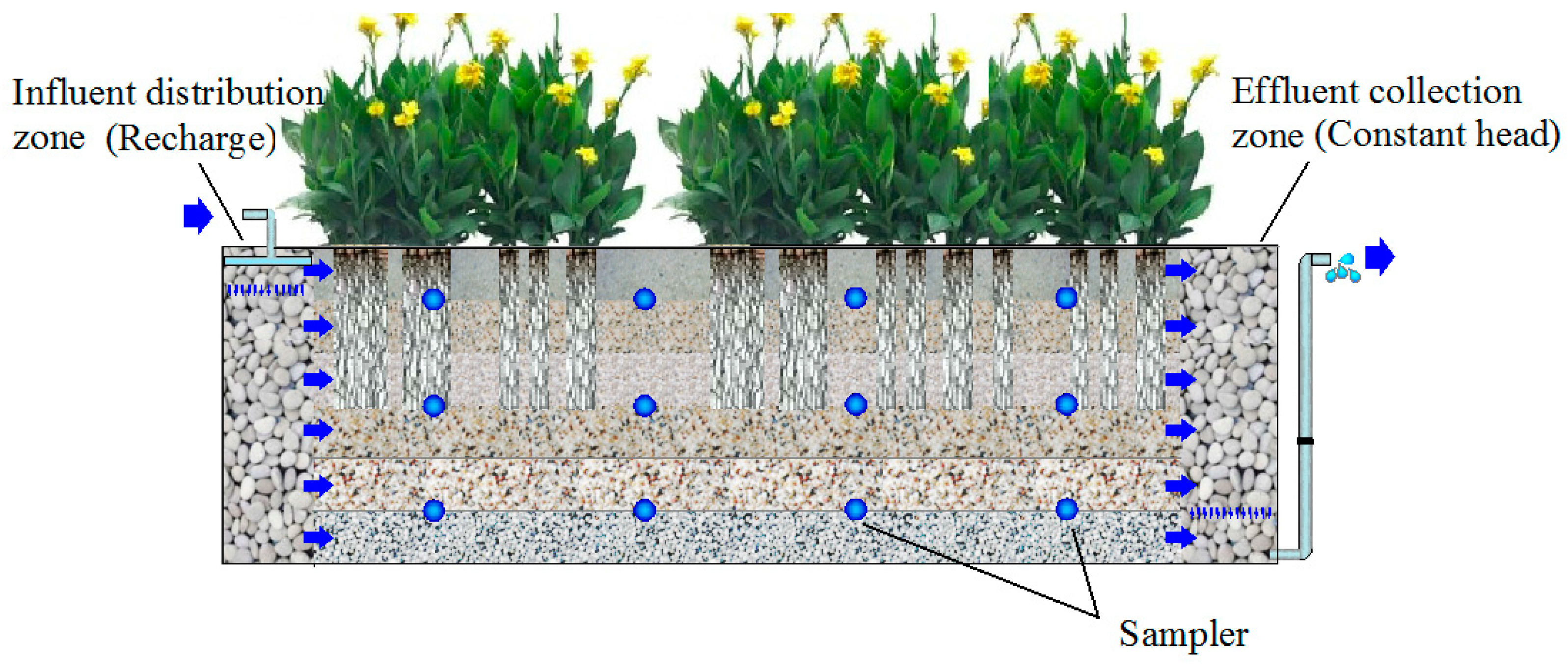
2.2.1. Experimental System Setup

Three parallel pilot-scale CWs were constructed according to the simulation results, with the dimensions of each system being 200 cm long, 120 cm wide, and 70 cm high (water depth of 60 cm) (Figure 3). The bed was composed of the distribution substrate, the main substrate and the collection substrate. The influent distribution zone and the effluent collection zone had the same dimensions of 20 cm × 120 cm × 70 cm (length × width × height) and were composed of gravel (30–80 mm in diameter) with a K value of 500 m/day.

According to the computer simulation results, the three CWs differed from each other in the configuration of their main filling substrate. The common materials used in the applied CW systems are sand or gravel, but not soil (particle diameter always below 0.1 mm). These materials with larger particle sizes can limit clogging problems and provide a high surface area for biofilm growth in CWs. Thus sand (for main CWs’ bed) and gravel (for inlet and outlet collection zone) were chosen in the present study. CW1 was a monolayer substrate configuration, filled with the original mixed quartz sand (0–6 mm) with a K of 65 m/day. CW3 and CW6 were multilayer substrate configurations, composed of the quartz sand with different grain sizes arranged in layers with the hydraulic conductivity of each layer increasing with depth. CW3 comprised three layers of equal thickness (20 cm). The K values of these layers were 26, 36, and 64 m/day from the surface to the bottom layer, respectively, and the corresponding diameters were 0–0.4 mm, 0.4–0.6 mm, and 1–3 mm. CW6 was built up by six equal layers of 10 cm each. From the top to the bottom, the grain sizes were 0–0.4, 0.4–0.6, 0.6–0.9, 1–2, 2–4, and 4–6 mm, with K values of 26, 36, 43, 55, 75, and 176 m/day, respectively. For each CW, a total of 12 polyvinyl chloride (PVC) pipes were placed at a distance of 0.4, 0.8, 1.2, and 1.6 m from the inlet at depths of 0.1, 0.3, and 0.5 m (Figure 3). All of the PVC pipes were equipped with valves accessible outside each system for water sampling.

The CWs were established in December 2012 at Guilin University of Technology, in southwest China. All the wetlands were planted with the macrophyte species Canna indica at the density of 20 individuals per square meter. The laboratory facility was protected from rain by a glass roof but was exposed to natural temperature variations and light exposure. The research was carried out with actual domestic wastewater pretreated by a septic tank to reduce the suspended solids contents. The CWs were operated with a nominal hydraulic retention time (HRT) of 36 h for most of their life span with a continuous flow rate of 0.72 m³/day. The experiment was conducted from January 2013 to September 2013, and the water temperatures ranged from 13 to 28 °C during the study period. The following ranges of factors were measured in the influent: the pH was 7.0–7.6, dissolved oxygen (DO) was 0.1–0.58 mg/L, oxidation-reduction potential (ORP) was −168 to −144 mV, concentration of chemical oxygen demand (COD) was 106–238 mg·L⁻¹, ammonia nitrogen (NH₄⁺-N) was 5–56 mg·L⁻¹, nitrate nitrogen (NO₃⁻-N) was 0.5–1.8 mg·L⁻¹, total nitrogen (TN) was 20–68 mg·L⁻¹, and total phosphorus (TP) was 0.8–7.3 mg·L⁻¹.

2.2.2. Water Sampling and Measurement

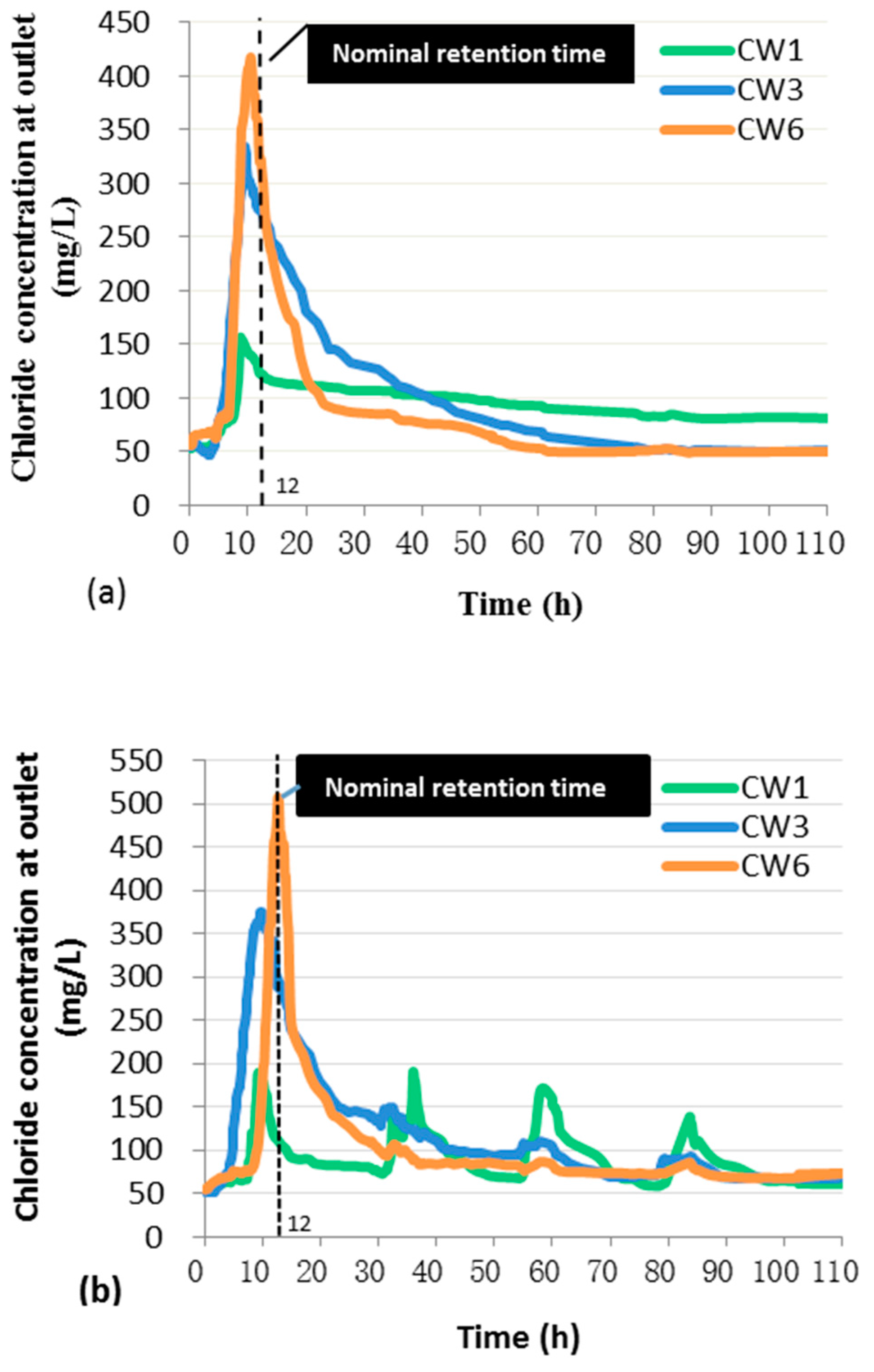
A total of 14 sampling locations were placed within each CW to provide repeatable points for water quality sampling, and these locations included the inflow, the outflow, and sample valves (Figure 3). The water from the influent and effluent pipe was sampled once a week to evaluate the effects of substrate configuration on pollutant removal. The contaminant concentration profiles were determined using the water sample measurements taken monthly from the sampling valves, and the resulting mean values were used to create isogram maps. During water sampling, the ORP and temperature were measured in situ using a HANNA HI9828 multiparameter portable meter. The sample was then analyzed immediately in the laboratory for COD, NH₄⁺-N, and TP by using standard methods (APHA, 1995).

2.2.3. Tracer Test

During the tracer tests, the wetlands were set a nominal hydraulic retention time (HRT) of 12 h. Tracer tests were conducted in each wetland for two sampling campaigns, January 2013 and September 2013 (absence and presence of growing vegetation, respectively), to analyze the hydraulic behavior of the CWs with different substrate configurations. The effects of plants on hydraulic performance were also evaluated by comparing the results of the two tracer tests. Each tracer test was conducted for 5 days by adding a single injection of sodium chloride solution (NaCl, 50 g/L) into the influent distribution zone (flow rate of 3 L/min, 4 min). Samples were taken from the effluent of each wetland and analyzed for chloride concentration every 1 h during the first 2 days and every 4 h during the following 3 days.

HRT was calculated according to the following ratio:

$$t_n=V/Q$$

(2)

where $Q$ is the flow rate (m³/day); and $V$ is the effective volume (m³).

Hydraulic efficiency ($\mathsf{\lambda }$) is defined by the ratio:

$$\mathsf{\lambda }=t_p/t_n$$

(3)

where $t_p$ is the time taken for the tracer to reach a peak in the experimental residence time distribution (RTD) curve (h), and $t_n$ is the nominal HRT (h). The hydraulic efficiency of a wetland can be considered high when $\mathsf{\lambda }>0.75$, satisfactory when $0.5<\mathsf{\lambda }<0.75$, and low when $\mathsf{\lambda }<0.5$ [16].

2.3. Statistical Analyses

Multiway analysis of variance (ANOVA) was performed to detect the differences in water flow distribution among CWs with different design factors. One-way ANOVA was used to detect the effect of substrate configuration on CW performances. A p-level ≤ 0.05 was used to indicate significant differences. The analysis was performed with SPSS.21 (SPSS—Boston, MA, USA: International Business Machines Corp, 2012). The isogram maps of COD, NH₄⁺-N, TP, and ORP data were created using MATLAB 7.0 (MathWorks, Natick, MA, USA) to identify data trends within the CWs.

3. Results and Discussion

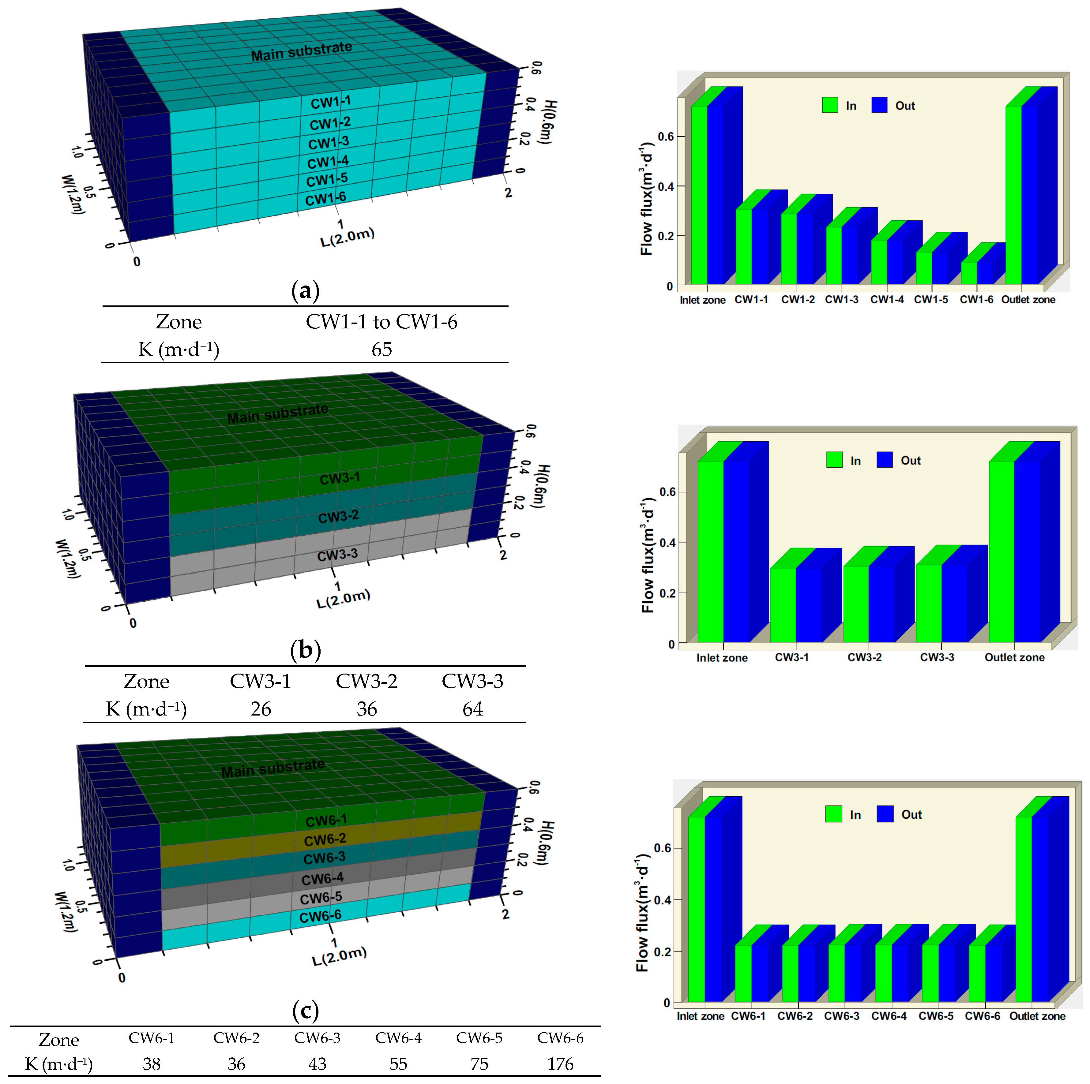
3.1. Effects of Design Parameters on Water Flow Distribution

The typical numerical simulation results are shown in Figure 4 for flux (water flow) distribution in each layer of CW models with different length-to-width ratios (3:1, 2:1, and 1:1), inlet/outlet-to-length ratios (1:5, 1:10, and 1:20), and substrate size configuration. The water flux in layer 1 (surface layer) was the highest among the six layers, and it decreased with increasing depth. Layer 6 (bottom layer) generally had the lowest flux compared with the other layers, particularly under monolayer conditions with a high K value (Figure 4c). This is consistent with previous research, which showed that preferential pathways exist in wetland beds, with water flowing mainly in the top layer and dead zones forming along the bottom of the bed, regardless of outlet position [17].

More evenly distributed water flow was correlated with higher length-to-width ratios in both mono- and multilayer CWs (Figure 4a). Higher length-to-width ratios increased the flux in the lower layers and reduced the flux in the upper layers, especially for layer 1. The length-to-width ratio of 3:1 was identified as the best of the three values tested for uniform flow distribution in both CW1 and CW3. Increased length-to-width ratios could shift the experimental retention time closer to the theoretical retention time, and result in higher plug flow and lower dead volume ratios due to the larger distance and the smaller cross-sectional area [17]. However, even under the best length-to-width ratio of 3:1, the flux in layer 1 was still significantly higher than that in layer 6 of CW1 (p < 0.05). In contrast, there were no significant differences among fluxes in the six layers (p > 0.05) in CW3 using the length to width ratio of 3:1. This indicates that substrate configuration was more important for achieving uniform flow distribution than the length to width ratio.

Increasing inlet/outlet-to-length ratio could also mitigate the non-uniformity of water flow in both mono- and multilayer CWs (Figure 4b). Lengthening the influent distribution and the effluent collection zones increased water flux in the bottom layers and reduced the flux in the surface layer, thereby allowing for more uniform water flow. The inlet or outlet length ratio of 1:5 was identified as the best of the three values tested for uniform flow distribution in both CW1 and CW3. However, the difference between layer 1 and layer 6 was still large in the monolayer structured CW1, even for the 1:5 ratio. In contrast, the differences among the six layers were not significant in CW3 under this same ratio. In view of this, even under the optimized inlet/outlet-to-length ratio, substrate configuration was more important for flow uniformity.

The effects of substrate size configuration on water flow distribution in the CWs are shown in Figure 4c. In the monolayer CWs (CW1), the differences among fluxes in the six layers increased with increasing values of substrate K. The increased flux in layer 1 from 0.22 m³/day (K of 50 m/day) to 0.37 m³/day (K of 200 m/day) corresponded to the decreased flux in layer 6 from 0.08 to 0.04 m³/day. Lower K values in monolayer CWs resulted in higher uniformity of flow distribution. Previous studies have indicated that finer porous media with lower K values could induce hydraulic behavior closer to an ideal plug flow system [9]. However, clogging has usually been found in CWs with substrates possessing K values below 20 m/day [18], thus, bigger substrate sizes with high K values are usually selected in applications to avoid clogging. Nonetheless, this increased substrate size may induce an uneven flow distribution, ultimately reducing the hydraulic performance and removal efficiency in monolayer CWs. In multilayer CWs, a structure using substrates with increasing K values from the surface to bottom layers could result in more uniform patterns of flow distribution (Figure 4a, CW 3, 50, 100, 200 m/day). In contrast, a structure using substrates with decreasing K values from the surface to bottom layers (Figure 4a, CW 3, 200, 100, 50 m/day) could result in more uneven distribution of the flow field, which was even less uniform than in the monolayer CWs. These results confirm that a rational arrangement of substrates according to the K values of porous media can reduce the formation of short-circuiting and dead zones [19]. Namely, composing the surface layer from low K value media can prevent water from traveling through the wetland bed on the fast-flow path, thus reducing short-circuiting in CWs. Also, filling the bottom layer with high K-value media (such as coarse porous media) will enhanced the water flux in the bottom layer, and offset the adverse effects of dead zones.

All of the three design parameters—length-to-width ratio, inlet/outlet-to-length ratios, and configuration of substrate size—had significant effects on the flow flux in each layer, and significant interactions were also observed among the three factors for the middle layers (2, 3, and 4). However, no two-way interaction was significant for the surface layer (layer 1). For the bottom layers (layer 5 and layer 6), significant interactions between configuration of substrate size and length to width ratios were observed (

Table 1. Results (F-ratios) of analysis of variance (ANOVA) of design parameters on water flux: length to width ratios (L), inlet/outlet to length ratios (I), and configuration of substrate size (S). Layer 1 represents the surface layer and layer 6 is the bottom layer.

Variable	L	I	S	L × I	L × S	I × S
Layer 1	109 *	378 *	430 *	0.5	0.7	3
Layer 2	42 *	507 **	183 *	1 *	16 *	8 *
Layer 3	215 *	248 *	300 *	22 *	15 *	14 *
Layer 4	163 *	56 *	173 *	10 *	8 *	8 *
Layer 5	202 *	17 *	394 *	6 *	26 *	3
Layer 6	2526 *	29 *	3376 *	4	315 *	5 *

Notes: * Indicates statistically significant values (p < 0.05), ** p < 0.01.

).

3.2. Model Optimization

Using the selected length-to-width ratio of 3:1 and inlet/outlet-to-length ratio of 1:5, one monolayer CW and two multilayer CW models (3-layer and 6-layer) were built to optimize for configuration of substrate size through the trial and error method. Furthermore, a monolayer CW1 with the K value of 65 m/day was built simultaneously as a control to check for the validity of the simulation results. The most optimized parameters for substrate size configuration in multilayer CWs to even out the distribution of water flow among the layers are shown in Figure 5. We identified two configurations of substrate size and layout that met the criteria of vertically uniform distribution of water flow: CW3 with three K values of porous media from surface to bottom (26, 36, 64 m/day) and CW6 with six K values from surface to bottom (38, 36, 43, 55, 75, and 176 m/day). The model results show that CW1 resulted in preferential flow along the surface, while the flow fluxes in CW3 and CW6 were vertically uniform.

3.3. Experimental Validation

3.3.1. Hydraulic Performance

The residence time distribution (RTD) curves of the tracer (chloride), based on the tracer concentration at the outlets for CW1, CW3, and CW6, were affected by absence (Figure 6a, winter) and presence of vegetation growth (Figure 6b, summer). When vegetation was inactive, the peak tracer concentration times ($t_p$) in CW1, CW3, and CW6 were observed at 8.7, 9.5, and 10.5 h, which are shorter than the nominal hydraulic retention time ($t_n$ of 12 h). The corresponding values of hydraulic efficiency ($\mathsf{\lambda }$) were 0.73, 0.79, and 0.88. The values of $\mathsf{\lambda }$ in the multilayer CWs were much higher than that in the monolayer CW. Also, more precisely divided layers (6 layers), which increases the hydraulic conductivity more gradually through the layers, were favorable for improving $\mathsf{\lambda }$. Moreover, the hydraulic performances of CW3 and CW6 can be considered to be high ($\mathsf{\lambda }>0.75)$. Even though the $\mathsf{\lambda }$ of CW1 was very close to 0.75, it should be noticed that the peak tracer concentration was clearly lower in CW1 than that in CW3 and CW6. Even after day 5 (120 h), the tracer could still be detected in the effluent of CW1. This observation suggests that in addition to the value of $\mathsf{\lambda }$, the amount of tracer recovered could be important in evaluating the hydraulic performances of the three CWs. Overall tracer recoveries were 62%, 85%, and 86% for CW1, CW3, and CW6, respectively. Some loss of the tracer was probably caused by the presence of dead zones at the bottom of the bed. Tracer elements that reach the dead zone may stay for longer periods because short-circuiting water flow, with narrow and continuously fast flow paths and longitudinal dispersion, will not exchange fluid with slow-flowing regions [20].

When vegetation was active during the summer, the peak tracer concentration times ($t_p$) in CW1, CW3 and CW6 were observed at 9.3, 9.8 and 11.7 h, and the hydraulic efficiencies ($\mathsf{\lambda }$) were 0.78, 0.82 and 0.98 for CW1, CW3 and CW6, respectively. The increased $\mathsf{\lambda }$ values when compared with the tests in winter indicate the positive effect of growing roots and rhizomes on the hydraulic performances of the three CWs. This has also been observed in previous research, where only the presence of plants seemed to help water to flow at least partially within the porous media; otherwise, water was shown to preferentially flow above the porous media, thus losing half the effective volume of the system [3,7,21]. The tracer recoveries of CW1, CW3, and CW6 were 72%, 82%, and 81%, respectively. For CW1, however, we observed 4 peaks and higher tracer recovery compared with winter values. This may have resulted from plant growth in CW1, which decrease K values of the surface layer substrate. The changes then promote smoother transport of the tracer ions from the bottom dead zones.

The experimental results support the simulation results, which indicated that a multilayer substrate structure with increasing K values from the surface to bottom could improve flow uniformity, in an indirect way. The direct measurement of the flow patterns inside the lab-scale pilot plants needed to be further investigated. The growth of roots and rhizomes could fill the spaces in the porous media in the surface layer, thus decreasing the K values in the surface layer, which would be beneficial for balancing the flow distribution in monolayer CWs. However, the effects of plants were not considered in the simulation models, and these effects should be investigated in future studies.

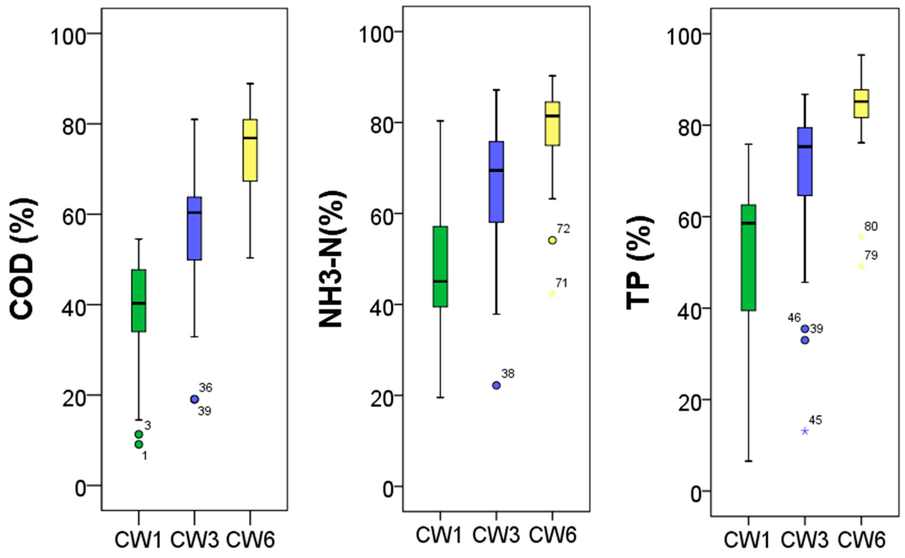
3.3.2. Overall Pollutant Removal Efficiencies

As shown in Figure 7, CW6 was significantly better at removing pollutants (72.9% for COD, 83.2% for TP, and 78.4% for NH₄⁺-N) than CW1 and CW3; it was especially better than CW1 (38.2% for COD, 50.5% for TP, and 46.9% for NH₄⁺-N). A significant effect of the substrate configuration on pollutant removal was observed (p < 0.05). The results indicate that multilayer configuration can achieve significantly higher removal rates of pollutants.

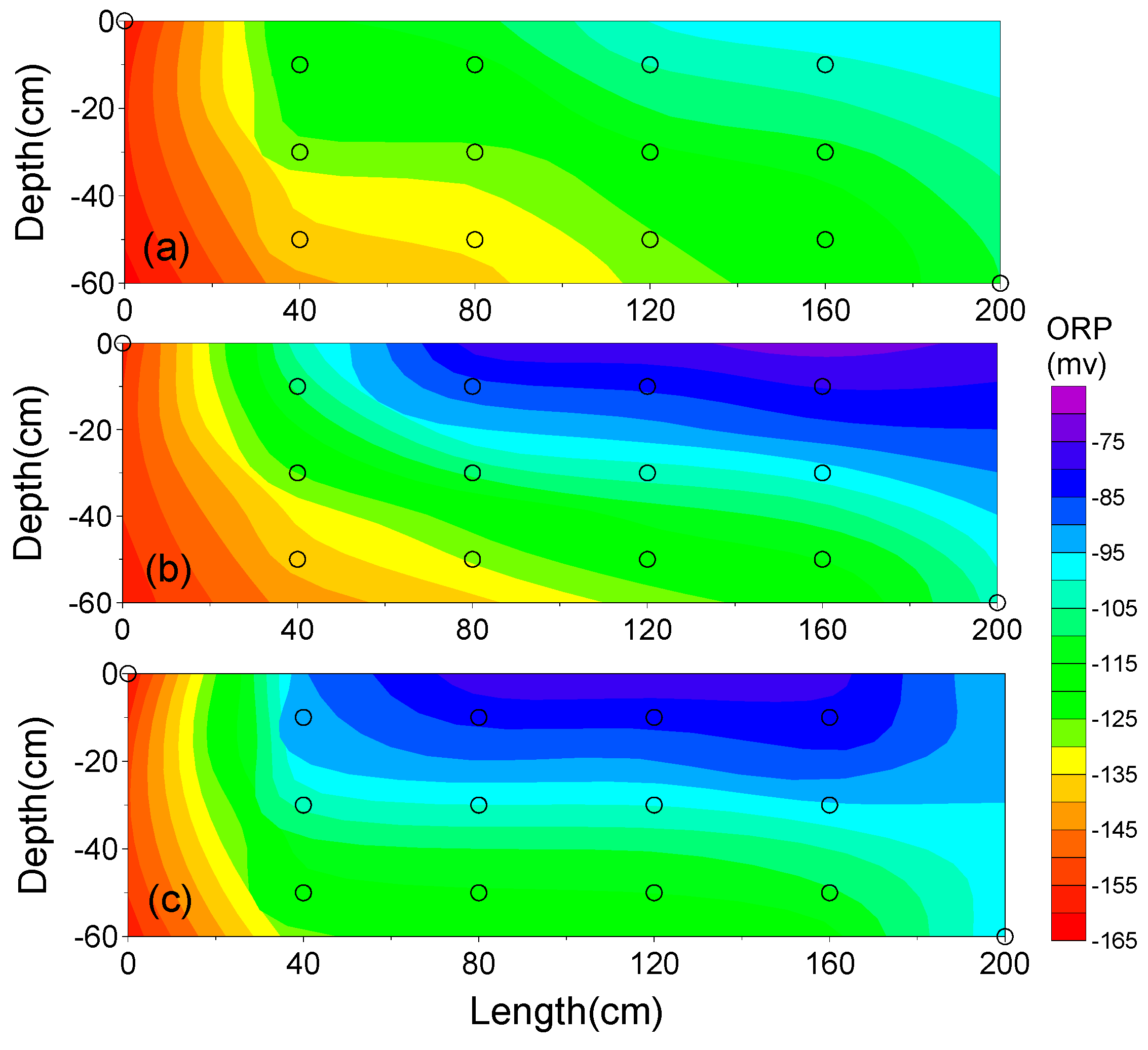
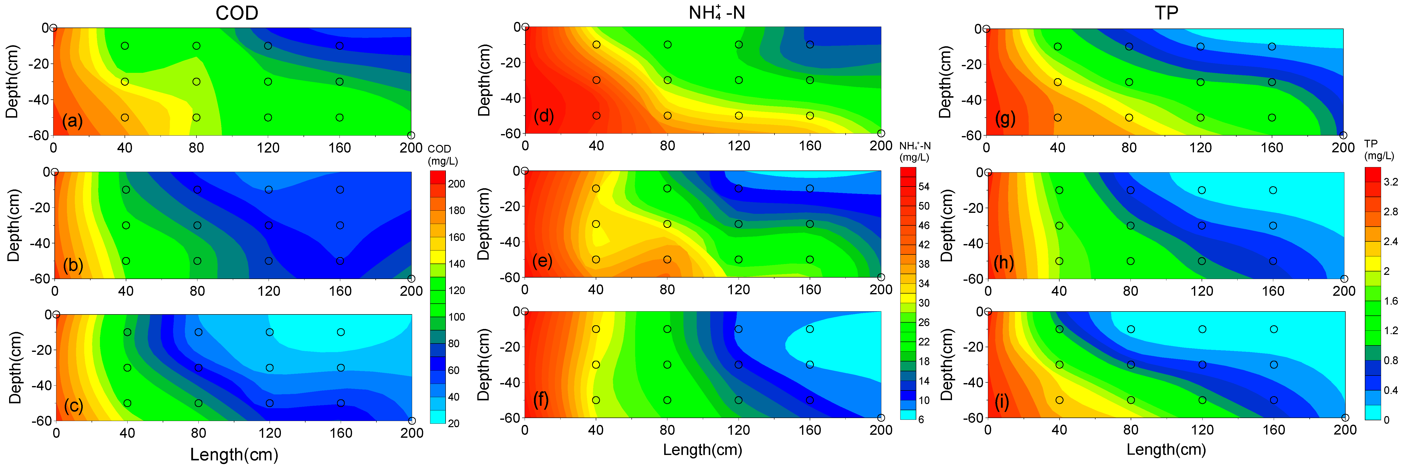
3.3.3. Water Quality and Spatial Distribution of Pollutants

The spatial distribution of ORP in the CWs is shown in Figure 8. The overall ORP in the substrates of the three CWs indicated anaerobic conditions (less than −70 mV). The mean ORP in the influent water was around −159 mV, whereas the values in the effluents of CW1, CW3, and CW6 were −110, −101, and −96 mV, respectively. The proportion of the bed volume with ORP above −100 mV did not differ significantly between CW3 and CW6, but the proportion was significantly larger than that in CW1. This result indicates that multilayer CWs can improve the ORP in the wetland bed by improving hydraulic performance.

The distributions of COD, NH₄⁺-N, and TP in the three CWs are shown in Figure 9. In CW1 (Figure 9a), the COD concentrations were generally lower in the upper than in the bottom layers. The higher COD concentration in the bottom could be attributed to the decline of ORP in dead zones. In CW3 (Figure 9b) and CW6 (Figure 9c), COD displayed a rapid and uniform horizontal decrease in concentration with the majority of removal occurring in the first half of the bed (0–1.0 m along the length). The minimum COD region (lower than 60 mg/L) was limited in CW1, and only appeared from 110 cm onwards to the outlet in the surface layer (from 0 to 20 cm depth), whereas the minimum COD region was more extensive in CW3 and CW6. A decrease of COD to lower than 60 mg/L occurred in nearly half of the whole cross-sectional area, especially on the surface of the bed near the outlet.

For NH₄⁺-N, the distributions showed similar trends to COD. The mean outlet NH₄⁺-N concentrations were 27, 16, and 9 mg/L in CW1, CW3, and CW6, respectively. In CW1 (Figure 9d), there was an obvious decrease of NH₄⁺-N in the upper layers. However, the degradation in the bottom layer was not significant. In CW3 (Figure 9e) and CW6 (Figure 9f), however, there was much faster removal of NH₄⁺-N, especially in CW6. The NH₄⁺-N removal rate in CW6 almost matched the trend found in horizontal plug flow. The minimum NH₄⁺-N region in CW6 (lower than 10 mg/L) was significantly larger than those in the other two CWs.

The mean outlet TP concentrations were 0.7, 0.3, and 0.2 mg/L in CW1, CW3, and CW6, respectively. In CW1 (Figure 9g), higher levels of TP remained in the bottom, reaching 1.5 mg/L at 160 cm along the flow path, whereas TP in upper layers at the same horizontal position was only 0.5 mg/L. The minimum TP region, lower than 0.5 mg/L, was obviously more extensive in CW3 (Figure 9h) and CW6 (Figure 9i) than in CW1. Especially in CW6, the minimum region appeared from 30 to 200 cm along the surface layer, which amounts to nearly half of the whole cross-sectional area. The spatial distribution of TP in the three CWs indicates the positive impact of multilayer CWs on TP removal. However, it should be noted that phosphorus removal largely depends on the adsorption by the substrate in CWs [22,23]. When the phosphorus concentration of the effluents exceeds a certain level, which was not reached in our experiments, this indicates that most of the substrate in the CW systems has reached adsorption saturation levels for phosphorus [24,25].

The patterns of spatial distribution and removal of pollutants in the three CWs indicate that the multilayer filling configuration facilitates full use of the bed space available and moderately reduces short-circuiting and the extent of the dead zone. The higher removal efficiencies of CW6 compared to CW3 showed that a more fine-scale division of layers favors higher CW performance.

4. Conclusions

The configuration of substrate size and layout played a crucial role in both the hydraulic behavior and pollutant removal efficiency of the CWs. A multilayer configuration with increasing hydraulic conductivity from the surface to bottom can make better use of the available bed space and moderately reduce short-circuiting and the extent of dead zones, significantly improving removal performance compared with the monolayer configuration. The similarity between the simulation and experimental results suggests that MODFLOW software can be effective in designing constructed wetland systems. This software could be adopted to design CWs and achieve uniform distributions of wastewater over the processing bed. However, the effects of precipitation, evapotranspiration, and plant growth on hydraulics should also be considered in future studies. Also, the hydraulic model can be extended with various process-based models derived from the various processes occurring in wetlands, such as adsorption/desorption and microbial degradation and conversion.

References

1. Brix, H.; Schierup, H.H.; Arias, C.A. Twenty years experience with constructed wetland systems in Denmark—What did we learn? Water Sci. Technol. 2007, 56, 63–68. [Google Scholar] [CrossRef] [PubMed]
2. Vymazal, J. The use of sub-surface constructed wetlands for wastewater treatment in the Czech Republic: 10 years experience. Ecol. Eng. 2002, 18, 633–646. [Google Scholar] [CrossRef]
3. Ríosa, D.A.; Vélez, F.T.A.; Pena, M.R.; Parra, C.A.M. Changes of flow patterns in a horizontal subsurface flow constructed wetland treating domestic wastewater in tropical regions. Ecol. Eng. 2009, 35, 274–280. [Google Scholar] [CrossRef]
4. Brovelli, A.; Carranza-Diaz, O.; Rossi, L.; Barry, D.A. Design methodology accounting for the effects of porous medium heterogeneity on hydraulic residence time and biodegradation in horizontal subsurface flow constructed wetlands. Ecol. Eng. 2011, 37, 758–770. [Google Scholar] [CrossRef]
5. Knowles, P.R.; Griffin, P.; Davies, P.A. Complementary methods to investigate the development of clogging within a horizontal sub-surface flow tertiary treatment wetland. Water Res. 2010, 44, 320–330. [Google Scholar] [CrossRef] [PubMed]
6. Knowles, P.; Dotro, G.; Nivala, J.; García, J. Clogging in subsurface-flow treatment wetlands: Occurrence and contributing factors. Ecol. Eng. 2011, 37, 99–112. [Google Scholar] [CrossRef]
7. Pedescoll, A.; Sidrach-Cardona, R.; Sa’nchez, J.C.; Carretero, J.; Garfi, M.; Be’cares, E. Design configurations affecting flow pattern and solids accumulation in horizontal free water and subsurface flow constructed wetlands. Water Res. 2013, 47, 1448–1458. [Google Scholar] [CrossRef] [PubMed]
8. Morales, L.P.; Franco, M.; Garvi, D.; Lebrato, J. Influence of the stone organization to avoid clogging in horizontal subsurface-flow treatment wetlands. Ecol. Eng. 2013, 54, 136–144. [Google Scholar] [CrossRef]
9. García, J.; Aguirre, P.; Barragán, J.; Mujeriego, R.; Matamoros, V.; Bayona, J.M. Effect of key design parameters on the efficiency of horizontal subsurface flow constructed wetlands. Ecol. Eng. 2005, 25, 405–418. [Google Scholar] [CrossRef]
10. García, J.; Chiva, J.; Aguirre, P.; lvarez, E.A.; Sierra, J.P.; Mujeriego, R. Hydraulic behaviour of horizontal subsurface flow constructed wetlands with different aspect ratio and granular medium size. Ecol. Eng. 2004, 23, 177–187. [Google Scholar] [CrossRef]
11. Kadlec, R.H.; Wallace, S. Treatment Wetlands; CRC Lewis Regional Relevance: Boca Raton, FL, USA, 2008. [Google Scholar]
12. Suliman, F.; Futsaether, C.; Oxaal, U.; Haugen, L.E.; Jenssen, P. Effect of the inlet–outlet positions on the hydraulic performance of horizontal subsurface-flow wetlands constructed with heterogeneous porous media. J. Contam. Hydrol. 2006, 87, 22–36. [Google Scholar] [CrossRef] [PubMed]
13. Liolios, K.A.; Moutsopoulos, K.N.; Tsihrintzis, V.A. Modeling of flow and bod fate in horizontal subsurface flow constructed wetlands. Chem. Eng. J. 2012, 200–202, 681–693. [Google Scholar] [CrossRef]
14. Ronkanen, A.K.; Kløve, B. Hydraulics and flow modelling of water treatment wetlands constructed on peatlands in Northern Finland. Water Res. 2008, 42, 3826–3836. [Google Scholar] [CrossRef] [PubMed]
15. Harbaugh, A. Modflow-2005, the US geological survey modular ground-water model—The ground-water flow process. In US Geological Survey Techniques of Water Resources Investigation Book; U.S. Department of the Interior, U.S. Geological Survey: Washington, DC, USA, 2005. [Google Scholar]
16. Persson, J.; Somes, N.L.G.; Wong, T.H.F. Hydraulics efficiency of constructed wetlands and ponds. Water Sci. Technol. 1999, 40, 291–300. [Google Scholar] [CrossRef]
17. Alcocer, D.J.R.; Vallejos, G.G.; Champagne, P. Assessment of the plug flow and dead volume ratios in a sub-surface horizontal-flow packed-bed reactor as a representative model of a sub-surface horizontal constructed wetland. Ecol. Eng. 2012, 40, 18–26. [Google Scholar] [CrossRef]
18. Pedescoll, A.; Uggetti, E.; Llorens, E.; Granés, F.; García, D.; García, J. Practical method based on saturated hydraulic conductivity used to assess clogging in subsurface flow constructed wetlands. Ecol. Eng. 2009, 35, 1216–1224. [Google Scholar] [CrossRef]
19. Schincariol, R.A.; Schwartz, F.W. An experimental investigation of variable density flow mixing in homogeneous and heterogeneous media. Water Resour. Res. 1990, 26, 2317–2329. [Google Scholar] [CrossRef]
20. Lightbody, A.F.; Nepf, H.M.; Baysb, J.S. Modeling the hydraulic effect of transverse deep zones on the performance of short-circuiting constructed treatment wetlands. Ecol. Eng. 2009, 35, 754–768. [Google Scholar] [CrossRef]
21. Suliman, F.; French, H.K.; Haugen, L.E.; Søvik, A.K. Change in flow and transport patterns in horizontal subsurface flow constructed wetlands as a result of biological growth. Ecol. Eng. 2006, 27, 124–133. [Google Scholar] [CrossRef]
22. Jiang, C.; Jia, L.; He, Y.; Zhang, B.; Kirumba, G.; Xie, J. Adsorptive removal of phosphorus from aqueous solution using sponge iron and zeolite. J. Colloid Interface Sci. 2013, 402, 246–252. [Google Scholar] [CrossRef] [PubMed]
23. Tuszynska, A.; Kolecka, K.; Quant, B. The influence of phosphorus fractions in bottom sediments on phosphate removal in semi-natural systems as the 3rd stage of biological wastewater treatment. Ecol. Eng. 2013, 53, 321–328. [Google Scholar] [CrossRef]
24. Vohla, C.; Kõiv, M.; Bavor, H.J.; Chazarenc, F.; Mander, Ü. Filter materials for phosphorus removal from wastewater in treatment wetlands—A review. Ecol. Eng. 2011, 37, 70–89. [Google Scholar] [CrossRef]
25. Dunne, E.J.; Coveney, M.F.; Marzolf, E.R.; Hoge, V.R.; Conrow, R.; Naleway, R.; Lowe, E.F.; Battoe, L.E. Efficacy of a large-scale constructed wetland to remove phosphorus and suspended solids from Lake Apopka, Florida. Ecol. Eng. 2012, 42, 90–100. [Google Scholar] [CrossRef]
Figure 1. Flow chart of the study approach using simulation and constructed wetlands (CWs).
Water 08 00556 g001
Figure 2. Three-dimensional view of the computational grid, boundary conditions and budget zones of the CW model domain.
Water 08 00556 g002
Figure 3. Longitudinal cross-section of each CW showing the sampling locations.
Water 08 00556 g003
Figure 4. Numerical simulation results of water flux distribution in each layer of the CWs with (a) different length-to-width ratios (3:1, 2:1, and 1:1); (b) different inlet/outlet-to-length ratios (1:5, 1:10, and 1:20); and (c) different K values.
Water 08 00556 g004
Figure 5. Setup of the in situ experiments, the assigned K values, and simulation results of CW1 (a); CW3 (b); and CW6 (c).
Water 08 00556 g005
Figure 6. Residence time distribution (RTD) curves of the tracer (chloride) based on tracer concentration at the outlets of CW1, CW3, and CW6, (a) without growing plants and (b) with growing plants.
Water 08 00556 g006
Figure 7. Correlation charts of removal efficiencies and substrate configuration for chemical oxygen demand (COD), total phosphorus (TP), and ammonium (NH4+-N).
Water 08 00556 g007
Figure 8. Profiles of oxidation-reduction potential (ORP) in CW-1 (a); CW-3 (b); and CW-6 (c).
Water 08 00556 g008
Figure 9. Spatial distribution of the pollutants COD (ac for CW1, CW3, and CW6, respectively), NH4+-N (df for CW1, CW3, and CW6, respectively), and TP (gi for CW1, CW3, and CW6, respectively) in the three experimental CWs.
Water 08 00556 g009