Article

Coastal Flooding Analysis in the Presence of REWEC1 Farms: A Case Study in Southern Italy

by
Francesco Aristodemo
1,*,
Giuseppe Tripepi
1 and
Pasquale Giuseppe Fabio Filianoti
2
1
Dipartimento di Ingegneria Civile, Università della Calabria, Via Bucci, Cubo 42B, 87036 Rende, Italy
2
RENEW—Marine Energy Laboratory, Department of Civil, Energy, Environmental and Material Engineering (DICEAM), Università Degli Studi Mediterranea di Reggio Calabria, Via Zhender, 1, 89122 Reggio Calabria, Italy
*
Author to whom correspondence should be addressed.
Water 2026, 18(4), 524; https://doi.org/10.3390/w18040524
Submission received: 10 January 2026 / Revised: 11 February 2026 / Accepted: 20 February 2026 / Published: 22 February 2026
(This article belongs to the Special Issue Coastal Flood Hazard Risk Assessment and Mitigation Strategies)

Abstract

Resonant Wave Energy Converter 1 (REWEC1) is a submerged caisson breakwater integrating a device designed to absorb incoming wave energy. Although the wave energy-extraction performance of this system and its hydraulic characteristics have been extensively investigated, its potential role in reducing coastal inundation, as an alternative to traditional rubble-mound breakwaters, has not yet been examined. In this context, the present study analyzes the mitigation effects on coastal flooding induced by the installation of REWEC1 barriers. The analysis focuses on the coast of Cetraro, located along the Tyrrhenian Sea in the province of Cosenza (Calabria, Southern Italy). The effectiveness of REWEC1 farms in reducing coastal flooding was assessed by considering fixed-air and no-air operation modes, as well as different spatial configurations. The input wave conditions were propagated in the nearshore using the SWAN model to simulate wave–structure interactions, while the XBeach model was employed to investigate coastal inundation processes based on the wave field behind the caissons, also accounting for Sea Level Rise (SLR). The results were evaluated in terms of maximum flooded areas and water penetration lengths along the emerged coast, as well as wave run-up and set-up along selected transects. To assess the robustness of the results, a sensitivity analysis was carried out by varying the transmission coefficients of the REWEC1 units within a plausible uncertainty range, and the corresponding variability in flooding indicators was quantified. The numerical results indicate a progressive reduction in these hydrodynamic response indicators as the spacing between adjacent REWEC1 devices decreases, and show that the relative mitigation performance of REWEC1 remains consistent when accounting for uncertainties in wave–structure interaction parameters. Further analyses were conducted to compare the effectiveness of REWEC1 farms with that of conventional rubble-mound breakwaters in reducing coastal flooding.

1. Introduction

Coastal flooding is one of the most significant natural hazards affecting low-lying coastal regions worldwide, with increasing frequency and severity driven by both climatic and oceanographic processes. Sea level rise, storm surges, and extreme wave events interact to increase water levels and inundate coastal areas, exposing ecosystems, populations, and infrastructures to growing risks [1]. Furthermore, several studies have shown that coastal inundation can have profound socioeconomic and environmental impacts, disrupting critical infrastructure, displacing communities, and degrading natural habitats that provide essential protective functions against meteo-marine events (e.g., [2]). In this context, advances in numerical modeling, data-driven approaches, and high-resolution mapping have improved the possibility of predicting and mitigating coastal flood impacts [3,4,5]. On the other hand, coastal flooding can usually be reduced through hard engineering measures [6], nature-based solutions [7], or adaptive coastal planning strategies [8].
Among the recent strategies to reduce the coastal risk due to the wave action, the use of Wave Energy Converter (WEC) farms represents a promising and suitable solution [9]. In addition to producing renewable energy to satisfy the growing energy demand and reduce carbon emissions [10], the possible employment of WEC for coastal protection, in the place of canonical hard and soft engineering solutions, can lead to a lowering of the Levelized Cost of Electricity (LCoE). Indeed, LCoE results in greater value for this kind of energy in comparison with conventional renewable energy sources (i.e., sun and wind) and fossil fuels (e.g., [11]). To improve the economic sustainability of WEC installations, several studies have highlighted their efficacy in reducing nearshore wave energy and, then, coastal erosion processes (e.g., [12,13,14,15]). Although a reduction in wave energy behind WEC is well documented, less attention has been paid to analyzing their impact in mitigating coastal flooding. To the authors’ knowledge, the only works related to this specific topic refer to Bergillos et al. [16,17], in which the authors investigated a WEC farm made of floating-type WaveCat devices for a gravel-dominated beach in Southern Spain. Attention was focused on studying how the geometrical effects of this wave farm influenced flooded areas and wave run-up under various meteo-marine scenarios. However, additional analyses are necessary to analyze the impact of various types of developed WEC on coastal hydrodynamic processes.
In this context, this study aims to analyze the performance of REWEC1 farms in reducing coastal flooding. REWEC1 belongs to the broad family of Oscillating Water Column (OWC) devices, which harness the motion of water and air inside a chamber to produce electrical energy [18]. The motivation for selecting this kind of WEC is due to its well-documented efficacy in capturing a significant rate of wave energy by field experiments [19,20] and numerical simulations [21,22,23,24]. Moreover, the integration into a classical breakwater allows REWEC1 to simultaneously provide coastal defense against wave action and produce renewable energy, with low environmental impact due to its submerged configuration. The present analysis was carried out along the coast of Cetraro, placed on the Tyrrhenian Sea in the province of Cosenza (Calabria, Southern Italy) and quite representative of the Calabrian Tyrrhenian coastal landscape. To analyze their effect on coastal inundations, various spatial arrangements of REWEC1 were tested, i.e., contiguous, with 10 m gaps, and with 20 m gaps, and compared with undisturbed conditions. To this end, this study employs a numerical modeling approach based on the coupling of the SWAN spectral wave model [25] and the XBeach hydro-morphodynamic model [26]. The two sets of wave conditions addressed different flooding regimes. Frequent coastal flooding was investigated under wave conditions representative of high-occurrence sea states, described by the 95th percentile (P95) of significant wave height H s , for which the REWEC1 was assumed to operate in fixed-air mode (active barrier), close to its resonance conditions. Conversely, extreme coastal flooding was analyzed under severe storm conditions characterized by design waves with return periods T = 25, 50, and 100 years, during which the REWEC1 was assumed to operate in no-air mode, behaving hydraulically as a conventional submerged breakwater. This distinction ensured physical consistency between the operational mode of the device and the adopted wave forcing. For both flooding regimes, SLR was incorporated by considering the high-emission RCP8.5 scenario projected for the year 2100, in order to assess the effectiveness of the REWEC1 under worst-case conditions. To account for uncertainties in the numerical estimation of the REWEC1 wave transmission coefficients, a sensitivity analysis was incorporated into the coastal flooding assessment. The numerically derived transmission coefficients were systematically perturbed by ±15%, and the resulting variability in flooding indicators was analyzed to assess the robustness of the results. To evaluate the effectiveness of REWEC1 as a coastal protection measure, its performance in mitigating coastal flooding was compared with that of conventional low-crested rubble-mound breakwaters, which represent a widely adopted solution in coastal engineering practice.
The paper is organized as follows. The main features of REWEC1 are illustrated in Section 2, paying attention to the assessment of its transmission and dissipation coefficients. Section 3 provides a brief description of the study area. Afterwards, the adopted numerical models are recalled in Section 4. The results obtained in terms of wave climate, wave propagation, and coastal flooding are discussed in Section 5, together with a comparison with classical rubble-mound breakwaters. The Section 6 closes the article.

2. Main Characteristics of REWEC1

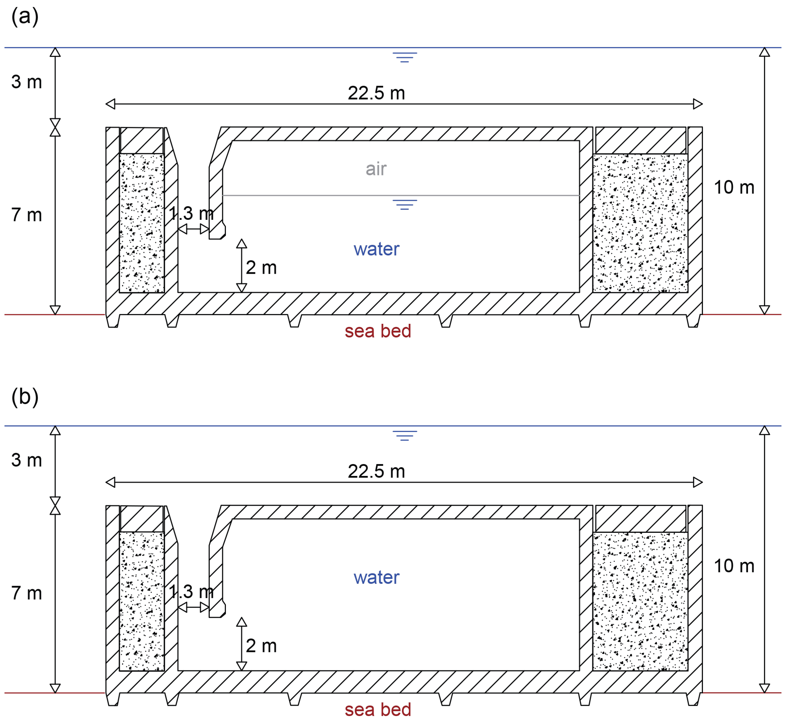
Among the different types of wave energy converters, the REWEC1 device was selected for the present study. A comprehensive overview of its main characteristics can be found in the work of Boccotti [18]. In general, the REWEC1 consists of a submerged caisson that simultaneously acts as a submerged breakwater for coastal protection and as a wave-energy absorber for electricity generation, thus functioning as an active barrier. Typically, this device can be deployed nearshore with a submergence of approximately 2–3 m below the Still Water Level (SWL). The REWEC1 is composed of multiple adjacent reinforced-concrete caissons, each featuring an internal U-shaped duct, a vertical arm facing the open sea with an upper opening, an internal air chamber acting as a pneumatic spring, and two lateral ballast cells filled with inert material to ensure structural stability (not involved in the energy absorption process). The operating principle is based on that of OWC devices, although with distinctive features. First, the wave pressure at the upper opening of the vertical duct induces oscillations of the internal water column. Second, the internal oscillations cause compression and decompression of the air within the internal chamber, which behaves as a mass–spring system. Third, by adjusting the air volume, the natural oscillation period of the internal water column can be tuned to match the incident wave period, allowing the system to operate under resonant conditions.
In the subsequent analyses aimed at assessing the mitigation effects of coastal flooding along the selected coastal site, reference is made to the design configuration proposed by Boccotti [18], in which the REWEC1 is installed at a water depth d = 10 m and has the following dimensions: height of 7 m, length of 22.5 m, and width of 20 m. Two different REWEC1 submerged breakwater configurations were adopted. The first is the fixed-air configuration, used when REWEC1 functions as an active barrier for electricity generation. This configuration was selected for recurrent wave conditions because it ensures stable operation and reliable wave energy attenuation under typical sea states. The second is the no-air configuration, in which the internal chamber is completely filled with water, resulting in increased structural stability under extreme wave conditions. This configuration is typical of winter conditions, during which the REWEC1 operates as a conventional breakwater rather than as an active wave-energy absorber. These two configurations were chosen to cover the full range of sea states considered in this study, from recurrent waves to extreme conditions, allowing an assessment of REWEC1 performance in both wave energy absorption and coastal flood mitigation. A schematic view of a REWEC1 device in fixed-air and no-air operation layouts is illustrated in Figure 1.
To characterize the hydraulic performance of REWEC1 devices operating in the fixed-air and no-air modes, and to support their implementation in the subsequent numerical simulations of wave–structure interaction, the transmission coefficient C T and the reflection coefficient C R were determined based on the numerical modelling approach developed by Filianoti and Piscopo [21].
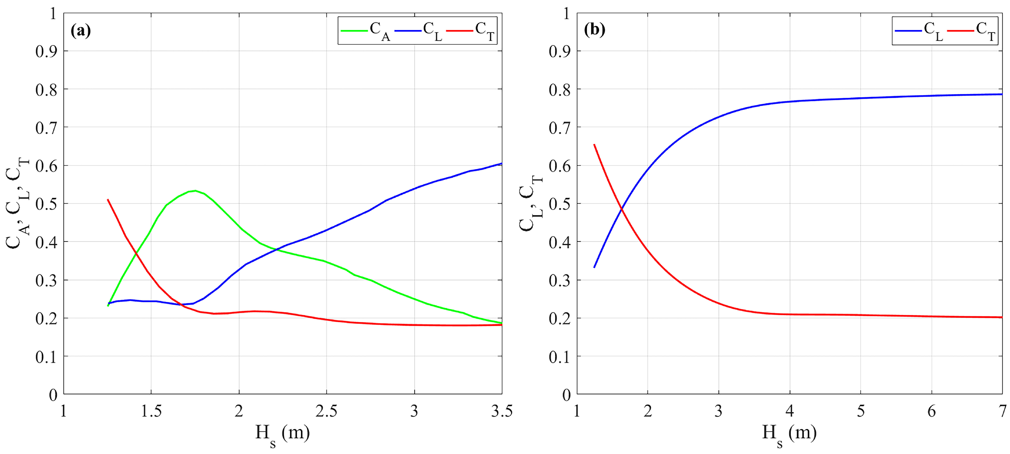
In the fixed-air operation mode, the above coefficients were derived from the range of H s reported by Filianoti and Piscopo [21], i.e., between 1 m and 3.5 m, as the most frequently occurring sea states at the selected coastal site fall within this range. While C T was evaluated directly, C R was determined based on energy balance considerations as a function of the absorption coefficient C A , the dissipation coefficient C L , and C T , specifically as C R = 1- C A - C L - C T . The trends of C A , C L , and C T as a function of H s are reported in Figure 2a. It can be observed that C A increases at low H s and decreases at high H s , reaching its maximum value at approximately H s = 1.75 m (resonance condition), while C L and C T exhibit an overall increase and decrease, respectively, with increasing H s . The resulting values of C R are very low, i.e., below 0.03.
In the case of a no-air operation layout, the numerical results provided by Filianoti and Piscopo [21], originally valid for H s up to 3.5 m, were extended to values up to 7 m, due to the extreme wave conditions at the selected case study. For given input values of H s and peak period T p , representative of irregular wave conditions, the fractions of reflected, transmitted, and dissipated wave energy resulting from interaction with the REWEC1 geometry were evaluated by applying a methodology that combines linear diffraction modeling, breaking-induced dissipation modeling, and energy balance principles, as detailed in Filianoti and Piscopo [21]. The outcome of this procedure is graphically reported in Figure 2b, which shows the trends of C T and C L as a function of H s . The reflection coefficient was subsequently computed as C R = 1- C T - C L . As shown in Figure 2b, C T decreases with increasing H s , from values of approximately 0.65 down to nearly asymptotic values slightly above 0.20, while C L progressively increases up to values slightly below 0.8. Wave reflection remains consistently low, with C R typically below 0.04.
Overall, the REWEC1 device exhibits low reflective behavior under both operating conditions, with wave energy being primarily absorbed in the fixed-air configuration and predominantly dissipated in the no-air configuration. This complementary behavior highlights the dual functionality of REWEC1, acting as an effective wave energy absorber under recurrent wave conditions and as a highly efficient wave energy dissipator under extreme sea states.

3. Study Area

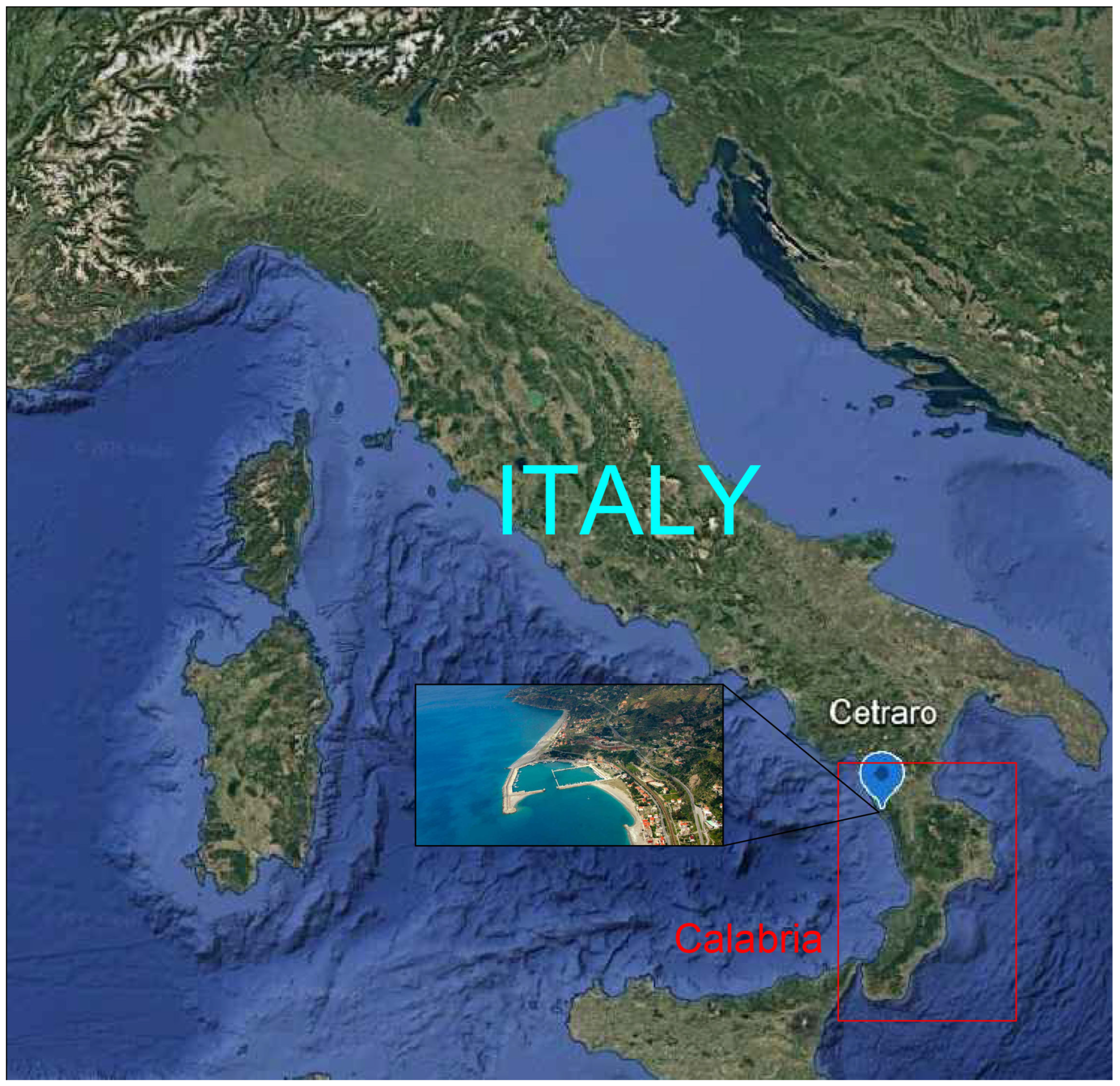
The study area used to analyze the performance of REWEC1 farms is Cetraro, a coastal town located along the central Tyrrhenian Sea in the province of Cosenza (Calabria, Southern Italy). Figure 3 shows a map of Italy with the position of the Calabria region and the Cetraro site. This site exhibits hydrodynamic and morphodynamic features typical of a microtidal, wave-dominated Mediterranean shore. The shoreline is predominantly linear to gently curvilinear and is characterized by sandy and gravel beaches, locally interspersed with coarse sediments and limited rocky outcrops, particularly near anthropogenic structures such as the harbor and coastal defenses in the Southern part [27].
From a hydrodynamic perspective, the Cetraro coast is exposed to the open Tyrrhenian basin, where the dominant wave climate is driven by north-westerly and westerly winds producing storm waves that significantly contribute to coastal processes [28]. Long-term wave climate analyses along the Calabrian coasts indicate that the Tyrrhenian side experiences heavier extreme wave conditions compared to the Ionian side, highlighting the importance of wave forcing in shaping coastal dynamics in this sector of the Mediterranean Sea [29,30].

4. Numerical Models

The wave propagation from deep waters to the studied nearshore region was conducted by applying the third-generation numerical model SWAN (Simulating WAve Nearshore), developed by the Fluid Mechanics Department of Delft University of Technology [25]. SWAN is a spectral model that simulates the evolution of two-dimensional wave spectra from deep water to shallow water depths. The model solves the spectral wave action balance equation N = E/f, where E is the spectral energy density and f is the frequency. In particular, both N and E are represented in the frequency–direction (f, θ ) domain. The modeling framework includes the main physical processes governing wave dynamics in coastal areas, such as wind wave generation, nonlinear wave–wave interactions, dissipation processes due to bottom friction and wave breaking, as well as nearshore propagation effects, including shoaling, refraction, diffraction, wave–current interaction, and transmission and reflection processes induced by wave–structure interaction.
The simulation of coastal flooding was provided by the hydro-morphodynamic numerical model XBeach (eXtreme Beach) [26]. This model allows the simulation of the response of coastal environments to extreme events such as storm surges and tsunamis. XBeach is an open-source model that explicitly resolves a wide range of coastal hydrodynamic and morphodynamic processes, including nearshore wave propagation, wave set-up and run-up, longshore and cross-shore sediment transport, seabed erosion and deposition, overwash and breaching processes, and, more generally, coastal flooding. From a hydrodynamic perspective, the XBeach model was applied in the “surf-beat” mode, in which waves are treated as a wave-group-scale process rather than resolving each individual wave cycle. In this framework, the wave motion is decomposed into a short-wave component (with periods shorter than 20 s), which is solved using an energy balance equation, and an infragravity-wave component (with periods longer than 20 s), which is resolved through the Shallow Water Equations. From a morphodynamic standpoint, seabed elevation changes are computed by solving the Exner sediment continuity equation, while the sediment transport rate is modeled using the Soulsby–Van Rijn formulation [31,32], and suspended sediment transport is simulated through an advection–diffusion equation for sediment concentration. XBeach has been successfully validated against laboratory experiments and real-world storm events in a wide range of coastal settings, including both sandy and defended coasts (e.g., [26,33,34,35]).

5. Results and Discussion

5.1. Wave Climate

For the purpose of analyzing coastal flooding scenarios in the absence and presence of the REWEC1 system protecting the Cetraro coast, a study of the coastal area was required in order to determine the deep water wave forcing conditions used as input. In this framework, historical wave data series derived from the MeteOcean hindcast database of the Department of Civil, Chemical and Environmental Engineering of the University of Genoa were considered (e.g., [36]). This dataset covers the entire Mediterranean basin, with a spatial resolution of 0.1273° in latitude and 0.09° in longitude, and a temporal resolution of 1 h. In particular, the used wave hindcast was validated by various Italian, Spanish, and Greek buoy measurements in the Mediterranean Sea, and used for a large number of analyses on wave climate (e.g., [37,38]).
In the present study, the reconstruction node no. 005659 was selected, located at a water depth of 473.3 m and characterized by the following coordinates: latitude 39.45° and longitude 15.874°. In particular, for the period from 1 January 1979 to 31 December 2018, the following synthetic wave parameters were extracted: significant wave height H s , peak period T p , and mean wave direction θ . The historical series were subject to a processing procedure aimed at quality control and the removal of inconsistent wave parameters [29]. The data efficiency, defined as the ratio between filtered and raw data, was equal to 99.68%. Since the reconstruction node is located at a distance of approximately 9 km from the Cetraro coastal area, no geographical transposition was required.
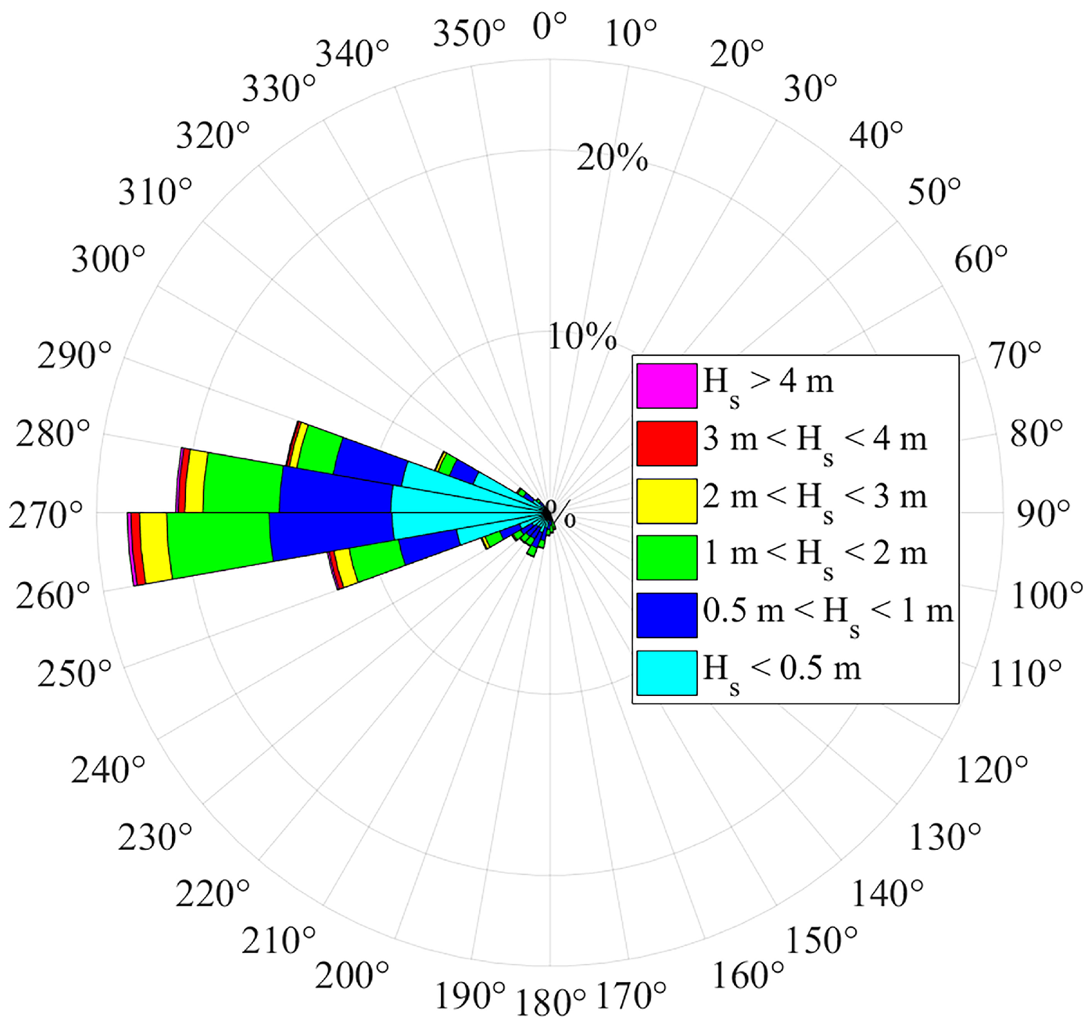
Figure 4 shows the directional wave rose derived from the historical wave data series of the selected reconstruction node, considering only sea states associated with the cross-shore exposure sector of the Cetraro coast (160°–320°). This figure illustrates the percentages of occurrence of wave events, classified into 10° directional sectors and different ranges of H s . The most frequent sea states are associated, in decreasing order, with the 260°–270°, 270°–280°, 280°–290°, and 250°–260° directional sectors, with occurrence percentages of 23.31%, 20.63%, 14.80%, and 12.47%, respectively. With reference to the H s intervals defined in Figure 4, the corresponding occurrence percentages are 45% for H s < 0.5 m, 28.36% for 0.5 m < H s < 1 m, 20.11% for 1 m < H s < 2 m, 4.61% for 2 m < H s < 3 m, 1.37% for 3 m < H s < 4 m, and 0.55% for H s > 4 m.
The fixed-air operation of the REWEC1 was investigated using offshore wave conditions corresponding to the 95th percentile (P95) of H s , since the nearshore propagation of this sea state to the installation depth of 10 m yielded values of H s close to the resonance condition of the device, associated with maximum energy absorption. The resulting H s value was 2.17 m.
In contrast, the no-air operation of the REWEC1 was analyzed using design waves with different return periods (T = 25, 50, and 100 years), representative of extreme sea states. To this end, the following procedure was carried out. First, the historical storm events impacting the Cetraro coastal area were identified using the Peaks-Over-Threshold (POT) method, by imposing a significant wave height threshold equal to 3.5 m. This threshold ensured a sufficient number of storm events for a robust estimation of the design waves. From the H s time series, storm events were identified when H s exceeded the above-mentioned threshold for a minimum persistence of 6 h and when the wave directions remained confined within an angular sector not exceeding 30° [39]. Storm intensity was characterized by the maximum significant wave height occurring during each storm event. Based on the highest number of storm events (2161), the 250°–280° directional sector was selected for the determination of the design waves. The determination of design waves was carried out using the method proposed by Goda [40], which considers both the Gumbel and Weibull probability distributions, with the Weibull shape parameter k set equal to 0.75, 1, 1.4, and 2. For the selected directional sector (250°–280°), the Weibull distribution with k = 1 was adopted, as it provided the best correlation between the significant wave height at the storm peak and the reduced variate associated with the non-exceedance probability. The values of H s associated with T = 25, 50, and 100 years are equal to 8.74 m, 9.23 m, and 9.72 m, respectively, for the 250°–280° directional sector.
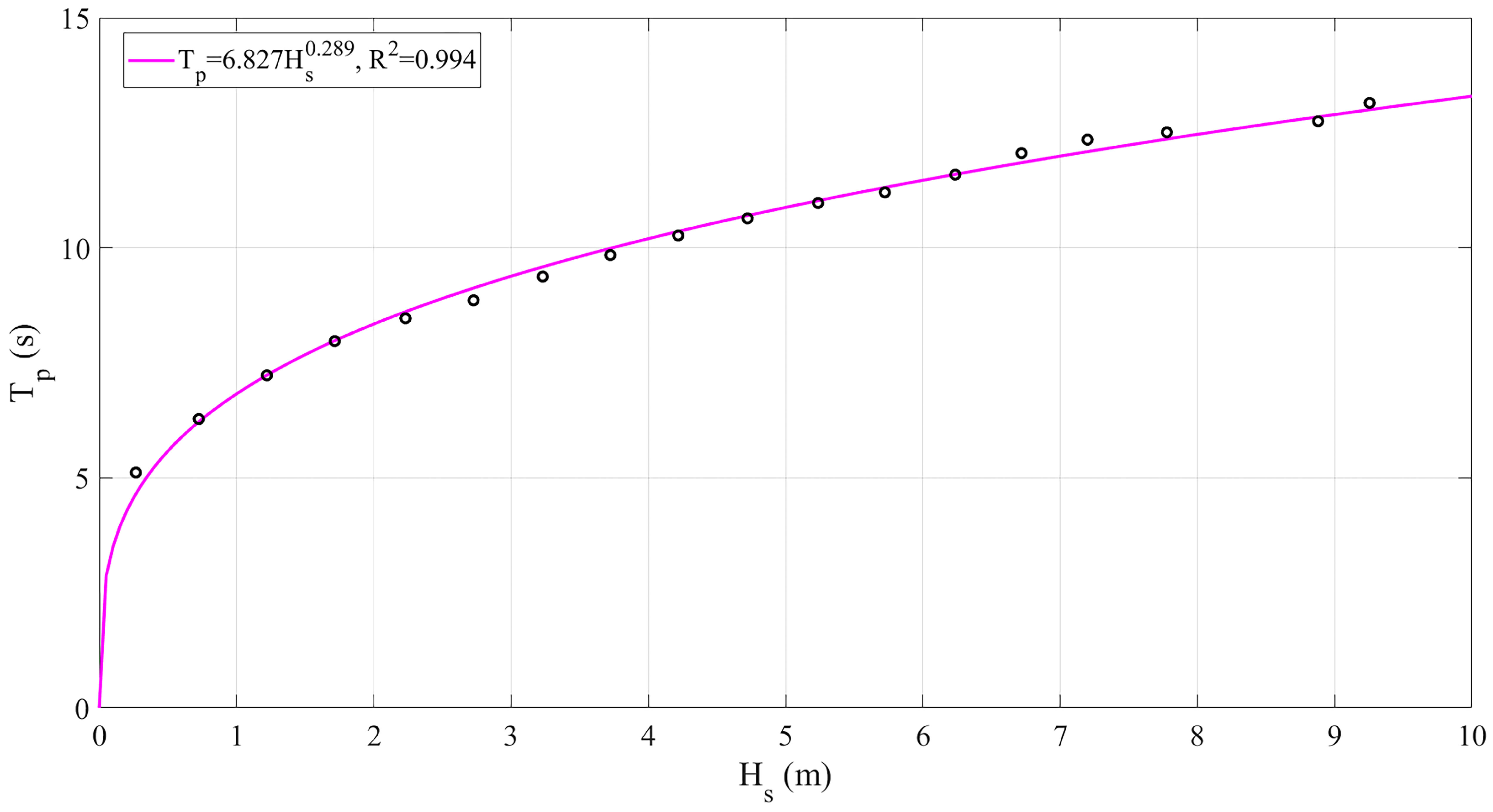
The peak wave period associated with P95 of H s was determined using a conditional statistical approach (e.g., [41]). Then, a representative T p of 8.7 s was derived from the resulting conditional distribution. The peak period values associated with the selected design waves within the chosen directional sector were derived by means of a power-law relationship of the form T p = α H s β . This relationship was obtained by interpolating the mean values of H s computed over 0.5 m intervals and the corresponding mean values of T p associated with the same intervals. As shown in Figure 5, the resulting curve was a good fit with the mean wave data with a correlation coefficient R 2 equal to 0.994. The calibrated parameters α and β were found to be equal to 6.827 and 0.289, respectively. Based on the calibrated power-law curve, the values of T p associated with H s for T = 25, 50, and 100 years were obtained, namely 12.77 s, 12.98 s, and 13.17 s.
The representative wave direction associated with the P95 of H s was determined by computing the circular mean of wave directions corresponding to all sea states with H s ≥ P95 [42]. Under this approach, the resulting θ was equal to 267.2°. The directions of the selected design waves were determined using the one-to-one quantile method [43], which allows the design wave to be associated with the real storm event whose significant wave height most closely matches the estimated extreme value. Therefore, the design wave directions were assumed to be equal to those of the observed event closest to the design condition. For the selected 250°–280° directional sector, the resulting θ values for T = 25, 50, and 100 years were 271.2°, 264.3°, and 263.7°, respectively.

5.2. Nearshore Wave Propagation

The offshore P95 of H s and the design waves with return periods T = 25, 50, and 100 years were propagated toward the nearshore zone in correspondence with the Cetraro coast using the SWAN model. The application of this model required the representation of the seabed morphology in front of the investigated coast. For the construction of an appropriate computational grid containing bathymetric information, bathymetric data were derived from nautical charts provided by the Italian Hydrographic Institute for deeper waters and from dedicated nearshore topo-bathymetric surveys with a spatial resolution of 0.5 m, carried out by the Department of Biology, Ecology and Earth Sciences of the University of Calabria (e.g., [27]). The spatial domain adopted for the SWAN computational grid was characterized by a length x = 10,800 m and a width y = 4200 m. The transformation of the bathymetric data into computational cells, with dimensions Δ x = Δ y = 15 m and assigned depth values, was performed using the software Surfer through a Kriging-type spatial interpolation [44].
Based on the offshore wave conditions and on the specific bathymetry of the study area, the SWAN model was initially applied in a baseline configuration without REWEC1 to derive, at the water depth of 10 m where these devices were placed, the characteristics of the incident wave field under undisturbed conditions. The input design waves were modeled using a two-dimensional JONSWAP spectrum with a spectral peak enhancement factor γ = 3.3 and a directional spreading parameter s = 10. From the SWAN propagation results obtained at the 10 m depth in the absence of REWEC1, the values of H s were derived to determine the transmission C T and reflection C R coefficients of the REWEC1 devices operating in fixed-air and no-air modes, as a function of the specific wave forcing. These parameters allow the hydraulic characterization of the devices in subsequent SWAN simulations, accounting for their presence. Although SLR modifies the relative submergence of submerged structures and may affect their hydraulic performance, in the present study, the transmission and reflection coefficients were kept unchanged. SLR was accounted for exclusively as an increase in the mean water level and superimposed on the wave conditions in the successive flooding simulations. This approach is consistent with common practice in coastal flooding assessments, where future SLR is incorporated as a shift in the hydrodynamic boundary conditions rather than through a reparameterization of wave–structure interaction processes (e.g., [45,46]). Therefore, the resulting analysis provides a conservative estimate of the mitigation performance of the REWEC1 devices.
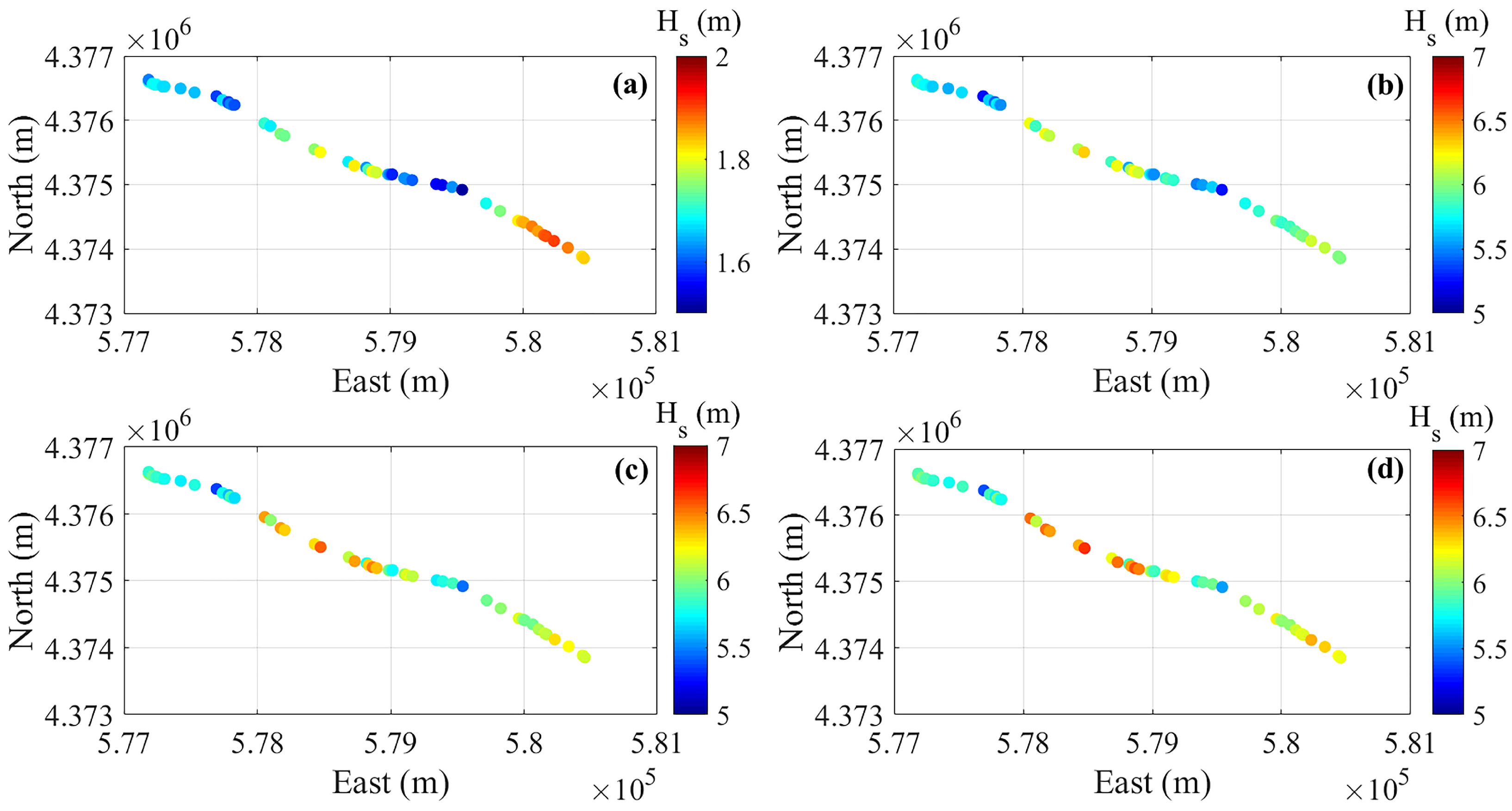
Figure 6 shows the variation of H s along the computational nodes closest to the 10 m depth contour, identified with a vertical tolerance of 0.05 m. The results refer to the P95 of H s (Figure 6a), characterized offshore by H s = 2.17 m, T p = 8.7 s, and θ = 267.2°; to the design wave with T = 25 years (Figure 6b), characterized offshore by H s = 8.74 m, T p = 12.77 s, and θ = 271.2°; to the design wave with T = 50 years (Figure 6c), characterized offshore by H s = 9.24 m, T p = 12.98 s, and θ = 264.3°; and to the design wave with T = 100 years (Figure 6d), characterized offshore by H s = 9.72 m, T p = 13.17 s, and θ = 263.7°. For the selected water depth, the values of H s range from 1.51 m to 1.90 m for the P95 of H s , from 5.29 m to 6.43 m for the design wave with T = 25 years, from 5.35 m to 6.53 m for the design wave with T = 50 years, and from 5.40 m to 6.64 m for the design wave with T = 100 years.
As shown in Figure 2, the values of C T and C L were derived as a function of the variability of H s at a water depth of 10 m for each wave attack and REWEC1 operating mode, while the corresponding values of C R were obtained from the energy balance, as described in Section 2. For the P95 of H s , C A oscillates between 0.43 and 0.53, C T oscillates between 0.21 and 0.31, C L between 0.24 and 0.31, and C R between 0.009 and 0.021. For the design wave with T = 25 years, C T oscillates between 0.203 and 0.207, C L between 0.778 and 0.784, and C R between 0.009 and 0.019. For the design wave with T = 50 years, C T oscillates between 0.202 and 0.206, C L between 0.780 and 0.785, and C R between 0.009 and 0.018. For the design wave with T = 100 years, C T oscillates between 0.201 and 0.205, C L between 0.781 and 0.787, and C R between 0.008 and 0.018. Owing to the relatively high values of H s associated with the selected design waves, only limited variations of these coefficients are observed.
The values of C T and C R enabled the characterization of the hydraulic performance of the REWEC1 devices, which can be represented in SWAN as rigid obstacles whose heads may be positioned within the computational domain at locations not necessarily coincident with the grid nodes [47]. In this framework, for each wave attack and at a water depth of 10 m (vertical tolerance of 0.05 m), three different spatial configurations of the REWEC1 devices were tested
  • Configuration 1: array of contiguous REWEC1 units, each 20 m long;
  • Configuration 2: array of 20 m long REWEC1 units with 10 m wide gaps;
  • Configuration 3: array of 20 m long REWEC1 units with 20 m wide gaps.
The choice of the gap length between devices for configurations 2 and 3 follows typical design criteria for detached rubble-mound breakwaters for coastal protection, according to which the gap length should range between 0.5 and 2 times the length of the barrier (e.g., [48,49]).
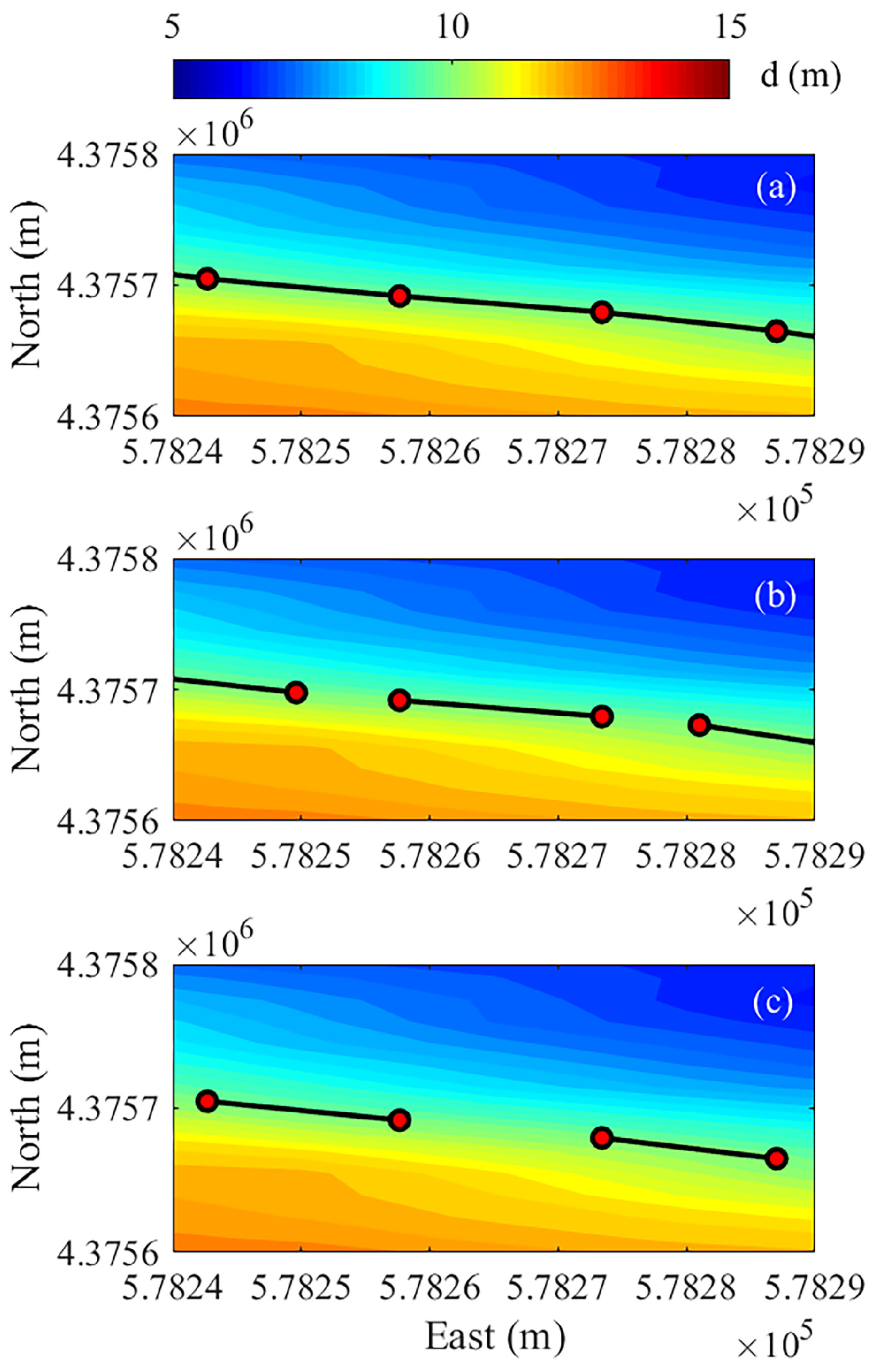
The obstacle arrangement procedure adopted to simulate the REWEC1 units within the SWAN computational domain consisted of four main steps. First, the target isobath at a water depth of 10 m was extracted from the bathymetric grid by identifying grid cells intersected by the selected depth contour and computing the corresponding contour segments through linear interpolation. Second, the contour segments were merged by removing duplicate nodes and assembling them into a graph structure, which was used to reconstruct continuous polylines representing the isobath geometry. Third, each polyline was parameterized along its curvilinear coordinate by computing the cumulative distance. Finally, obstacles were generated by sampling the curvilinear abscissa and defining straight segments with a fixed length of 20 m, separated by either zero gap (continuous configuration) or constant gaps of 10 m and 20 m. This procedure was specifically designed to generate obstacle geometries suitable for implementation in the SWAN model, ensuring a consistent representation of obstacle length, spacing, and alignment with the local isobath geometry. In the SWAN model, the values of C T and C R obtained at a water depth of 10 m as a function of H s were assigned to the individual obstacles representing the REWEC1 devices, based on their positioning within the three tested spatial configurations. A representative detail of the three adopted REWEC1 configurations, including the bathymetry around the 10 m water depth, is shown in Figure 7.
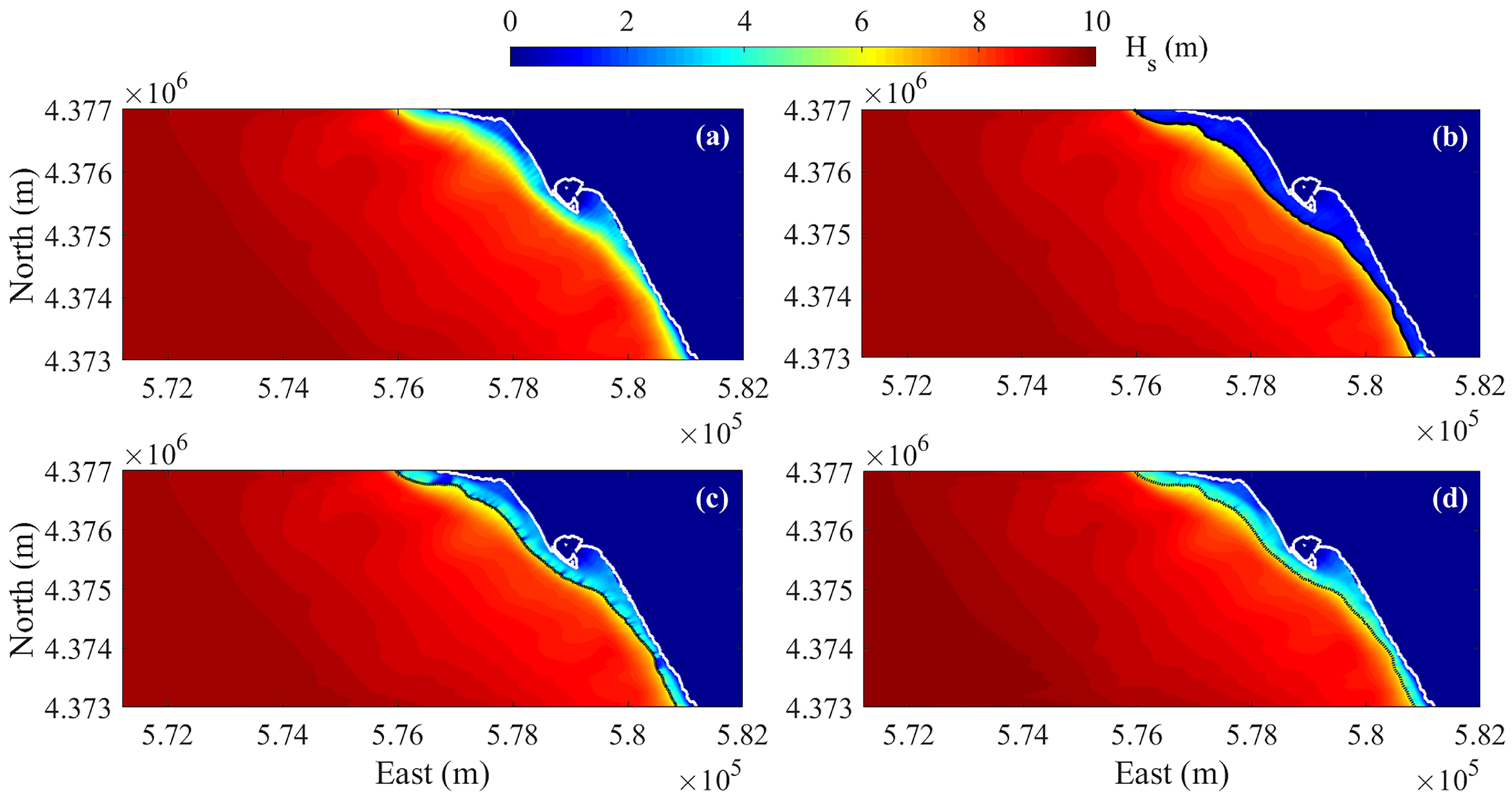
The results of the SWAN numerical simulations are shown in Figure 8 in terms of the spatial variation of H s for the representative and most variable case, corresponding to the design wave with T = 100 years. The figure compares undisturbed conditions (without REWEC1), configuration 1 (contiguous REWEC1), configuration 2 (REWEC1 with 10 m gaps), and configuration 3 (REWEC1 with 20 m gaps). The shoreline is indicated by a white line, whereas, in the subplots referring to the three REWEC1 spatial configurations, the units are highlighted by black lines. As observed, the attenuation of H s in the lee of the REWEC1 devices varies depending on their spatial configuration, in comparison with the baseline configuration characterized by undisturbed conditions (Figure 8a). In configuration 1 (Figure 8b), where the REWEC1 units are arranged contiguously, a substantial reduction of H s (approximately 80% immediately downstream of the devices) is observed, as a consequence of transmission coefficients on the order of 0.2. Due to the contiguous arrangement of the devices, this attenuation is spatially distributed in a nearly uniform manner in their lee. In configuration 2 (Figure 8c), where the REWEC1 units are arranged with 10 m wide gaps, the H s values in the sheltered area exhibit a marked spatial heterogeneity. The presence of 10 m gaps between adjacent REWEC1 modules allows part of the wave energy to propagate downstream through diffraction processes. This modular arrangement with gaps implies a combined effect of energy dissipation due to wave breaking at the modules and wave propagation through the gaps. Overall, the significant wave height is, on average, reduced within the area protected by the REWEC1 array. In configuration 3 (Figure 8d), characterized by 20 m wide gaps between the REWEC1 units, a greater spatial homogeneity of H s values downstream of the devices is observed compared to the case with 10 m gaps. The increased homogeneity of the wave field in the lee of the REWEC1 array with wider gaps is a direct consequence of the dominance of diffraction and wave propagation processes. As the gap width increases, the portion of the wave front passing through the gaps spreads more effectively, dispersing energy over a wider area and with a larger angular extent. In this context, the interference between waves diffracted from the two ends of a gap and from successive gaps tends to overlap more uniformly, smoothing the differences between the area immediately behind the REWEC1 units and the area immediately behind the gaps, where maximum wave transmission occurs.
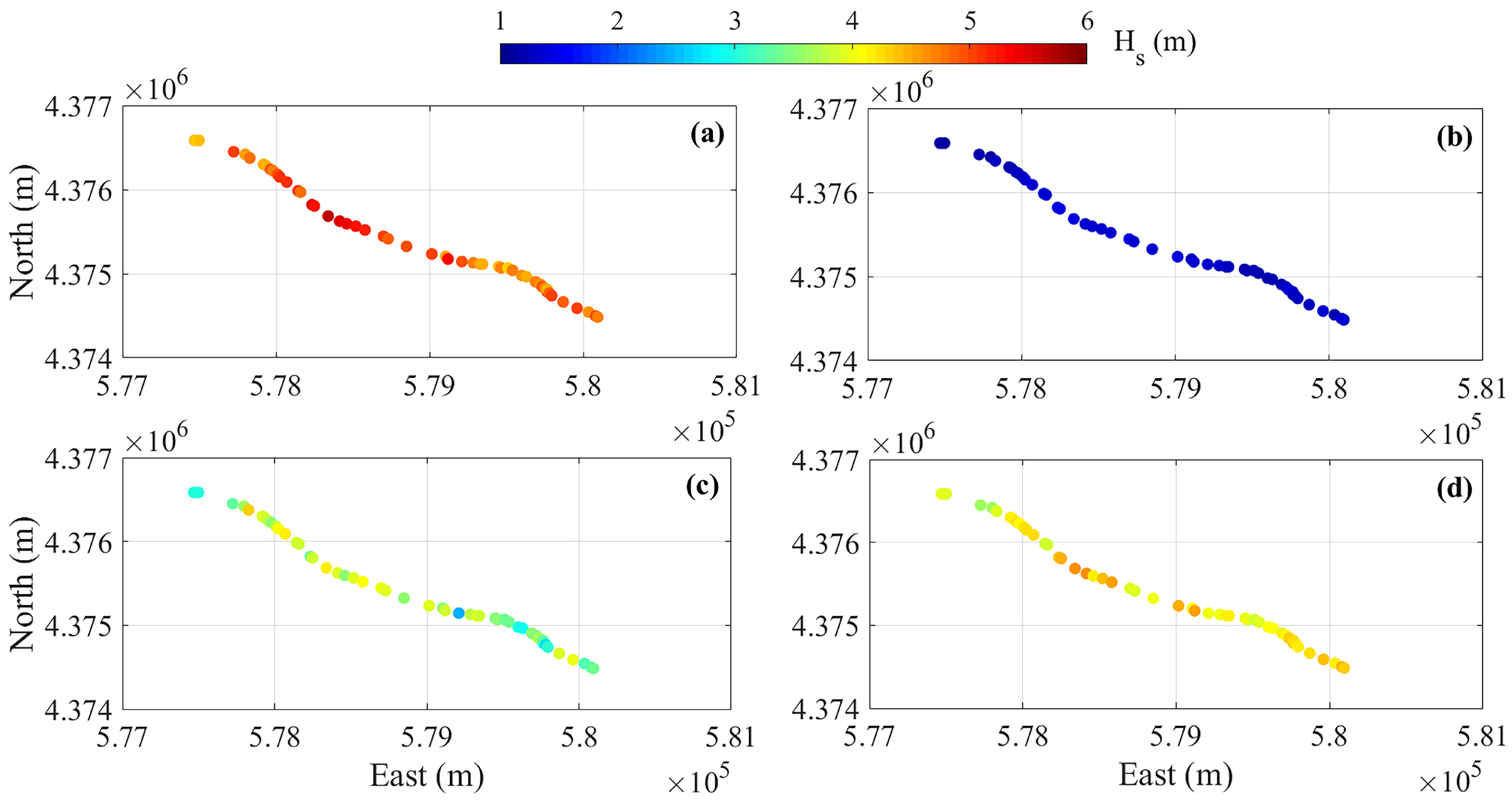
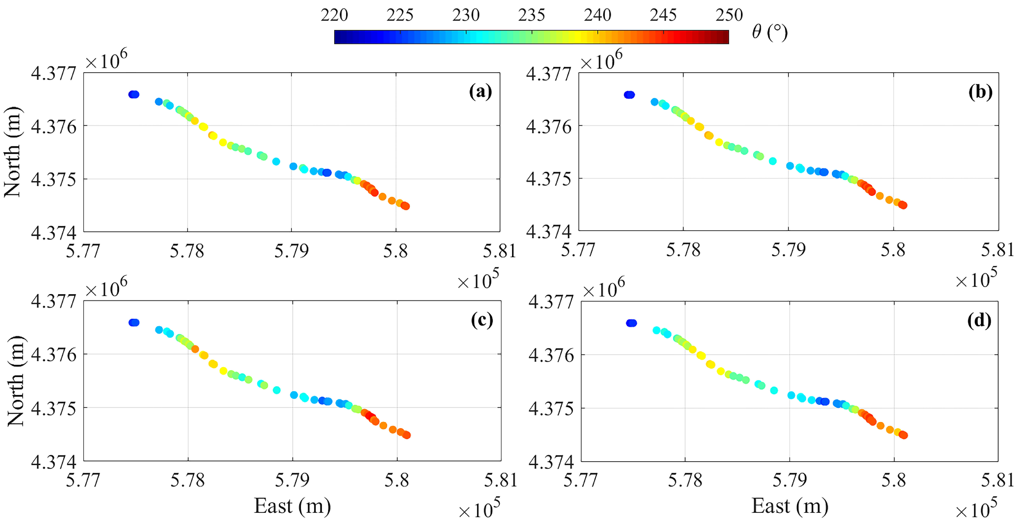
However, the SWAN numerical model does not allow for the simulation of coastal flooding processes. For this reason, a second numerical model was required to investigate these processes and assess the impact of REWEC1 farms on mitigating coastal flooding risk. In the present study, the SWAN results, obtained both in the absence and in the presence of REWEC1 under the different spatial configurations, were provided as input to the subsequent XBeach hydro-morphodynamic model capable of simulating coastal inundation processes. Considering the placement of the REWEC1 devices at a water depth of 10 m, the values of H s , T p , and θ simulated by SWAN under fixed-air and no-air operating modes, and for different configurations (absence of REWEC1, contiguous REWEC1, REWEC1 with 10 m gaps, and REWEC1 with 20 m gaps) were extracted in the lee of the devices, i.e., at a depth of 7 m, to account for the specific wave field resulting from the interaction with the devices. Considering the design wave with T = 100 years as a representative case, Figure 9 shows the trends of H s at a set of computational nodes closest to the 7 m depth contour, identified within a vertical tolerance of 0.05 m. A strong variation of H s among the different configurations can be observed, with values progressively decreasing from the configuration without REWEC1 (Figure 9a) to the configuration with contiguous REWEC1 units (Figure 9b). Configurations characterized by REWEC1 units with 10 m gaps (Figure 9c) and 20 m gaps (Figure 9d) exhibit a higher spatial variability of H s values along the computational domain compared to the other configurations. Concerning the mean wave direction θ (Figure 10), the spatial variability among the different configurations is fairly similar, although slightly larger oscillations are observed in the presence of REWEC1 devices with gaps (Figure 10c,d). As for the peak period T p , it remains unchanged at the 7 m depth with respect to offshore conditions in the absence of REWEC1, whereas in the presence of REWEC1 it exhibits a slight increase (ranging between 1% and 2%). This behavior is because the devices tend to attenuate high-frequency spectral components to a relatively greater extent than low-frequency components, producing a slight shift of the spectral peak toward longer periods.

5.3. Coastal Flooding

The results in terms of significant wave height H s , peak period T p , and mean wave direction θ at a water depth of 7 m, obtained for the fixed-air and no-air operating modes of REWEC1, were used as input to the hydro-morphodynamic numerical model XBeach [26]. To limit the number of numerical simulations while preserving a conservative assessment of future conditions, a single high-end SLR scenario was considered. The RCP8.5 projection for the year 2100 was adopted and superimposed on the wave-induced flooding scenarios, including frequent wave conditions (P95 of H s ) under fixed-air operation and extreme storm events with 25-, 50-, and 100-year return periods under no-air operation. SLR projection under the RCP8.5 scenario was obtained from the NASA Sea Level Projection Tool (sealevel.nasa.gov/ipcc-ar6-sea-level-projection-tool), which provides access to global and regional sea level projections from the IPCC Sixth Assessment Report [50]. Based on the IPCC RCP8.5 projections, a SLR of 0.78 m was found for the study area.
The first step in the application of the XBeach model consisted of defining the computational grid using the Delft3D software package [51]. As for the SWAN model, grid construction was based on topographic and bathymetric data derived from nautical charts provided by the Italian Hydrographic Institute and from dedicated nearshore topo-bathymetric surveys conducted by the Department of Biology, Ecology and Earth Sciences of the University of Calabria (e.g., [27]). In addition, the topography of a portion of the emerged coast was reconstructed using LIDAR data available from the National Geoportal of the Italian Ministry for the Environment and Energy Security (gn.mase.gov.it/portale/home), with a spatial resolution of 1 m.
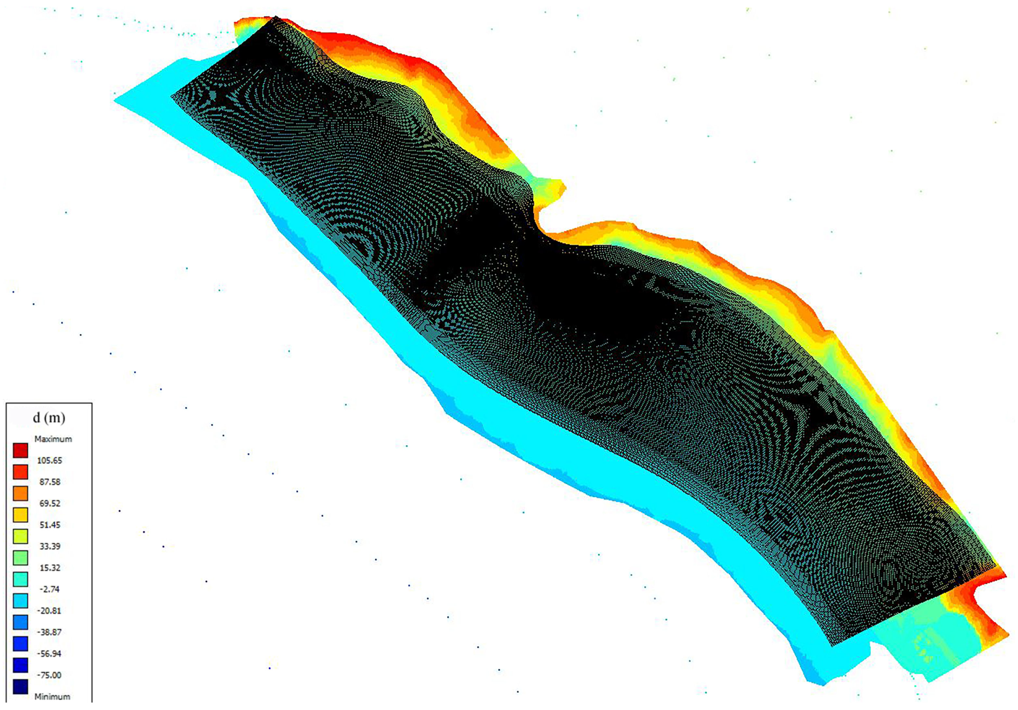
Based on these datasets, a curvilinear computational grid was generated, extending from the −7 m depth contour offshore to elevations inland exceeding the maximum expected flooding levels. The grid consists of 364   ×   721 computational nodes, with spatial resolution varying between 10 m and 1 m. Grid refinement was applied in the vicinity of the shoreline in order to achieve a higher level of detail in the simulation of nearshore hydrodynamic processes. Figure 11 shows the topography of the emerged and submerged coastal areas, together with the curvilinear grid adopted for the Cetraro coast to run XBeach simulations.
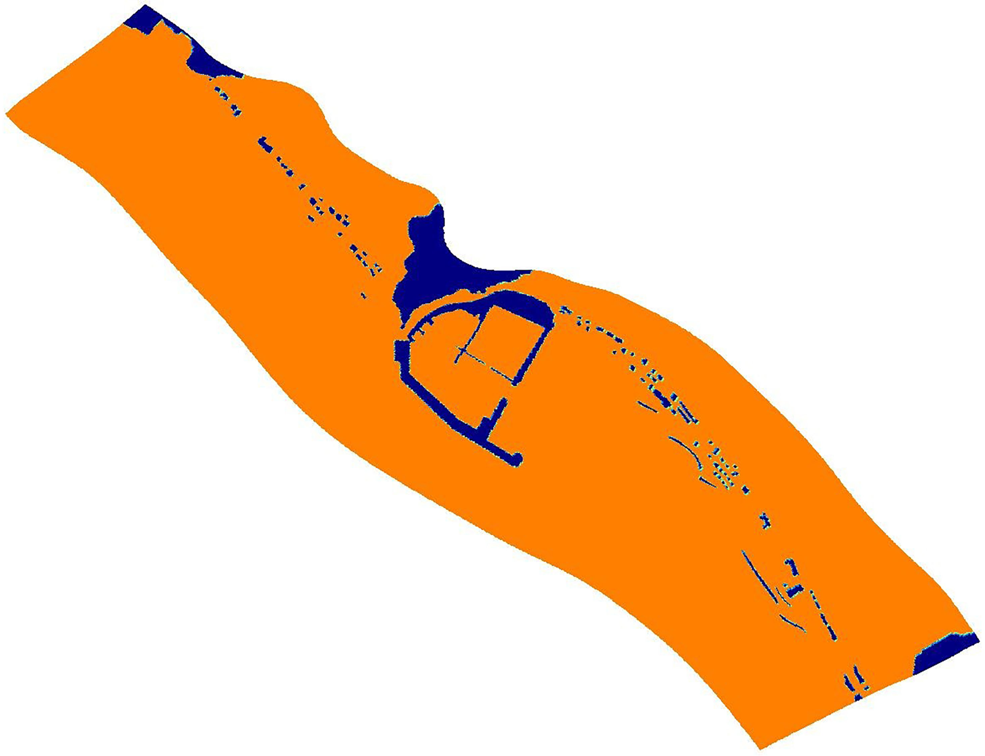
To optimize the numerical simulations performed with XBeach, particular care was devoted to the definition of non-erodible computational cells, representing the port infrastructure of Cetraro, the breakwaters located South of the port, various coastal civil infrastructures, and rocky outcrops of the emerged coast. A detailed representation of these elements is provided in Figure 12.
The offshore boundary conditions for XBeach were specified at each grid node along the offshore boundary of the computational domain by interpolating the wave parameters ( H s , T p , and θ ) obtained from the SWAN simulations at a water depth of 7 m. As for the SWAN model, the input two-dimensional JONSWAP spectrum was defined using γ = 3.3 and s = 10 . To characterize the sediment properties of the study area, a median grain size D 50 = 0.49 mm and a 90th percentile grain size D 90 = 1.5 mm were adopted. These values were derived from a recent granulometric survey campaign carried out by the Municipality of Cetraro within a project aimed at assessing the morphodynamic functionality of the port.
The duration of the XBeach simulations, aimed at analyzing maximum coastal flooding both in the absence and presence of REWEC1 devices, was set equal to 6 h in order to balance physical realism and computational cost. Preliminary analyses showed that longer simulation times did not lead to significant changes in the main engineering-relevant variables related to coastal flooding, such as maximum inundated areas, maximum inland water penetration, and wave set-up and run-up values.
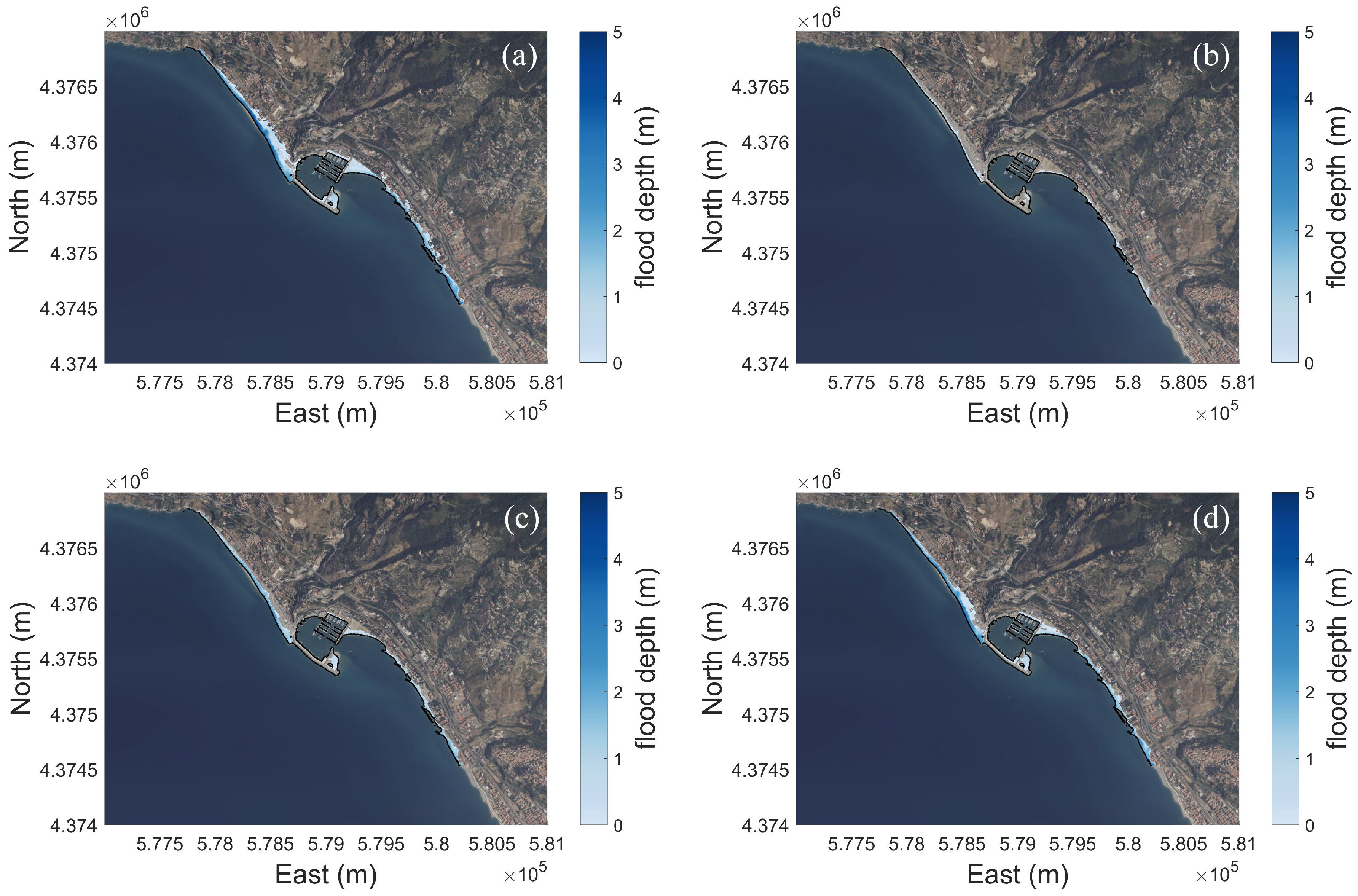
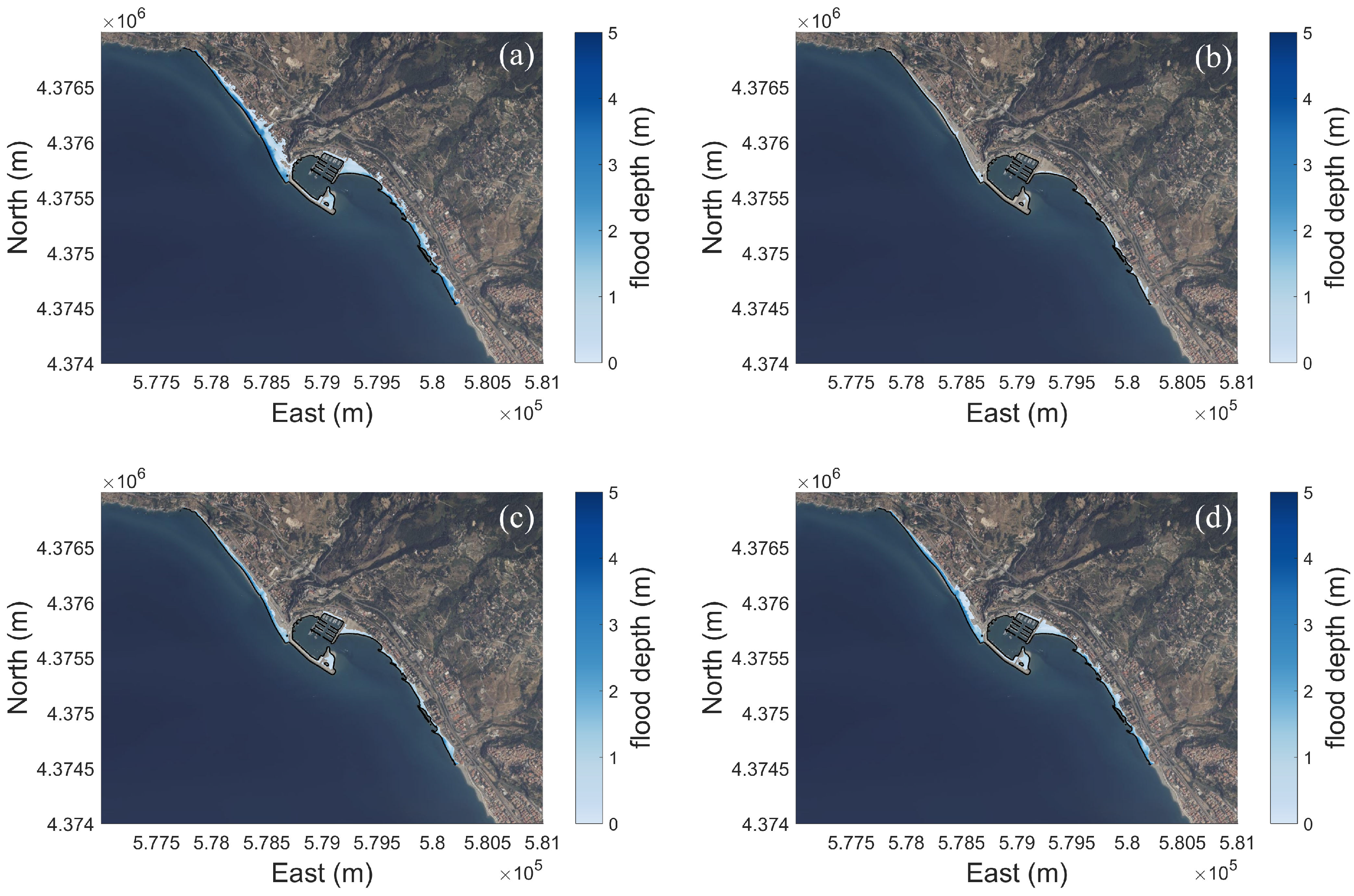
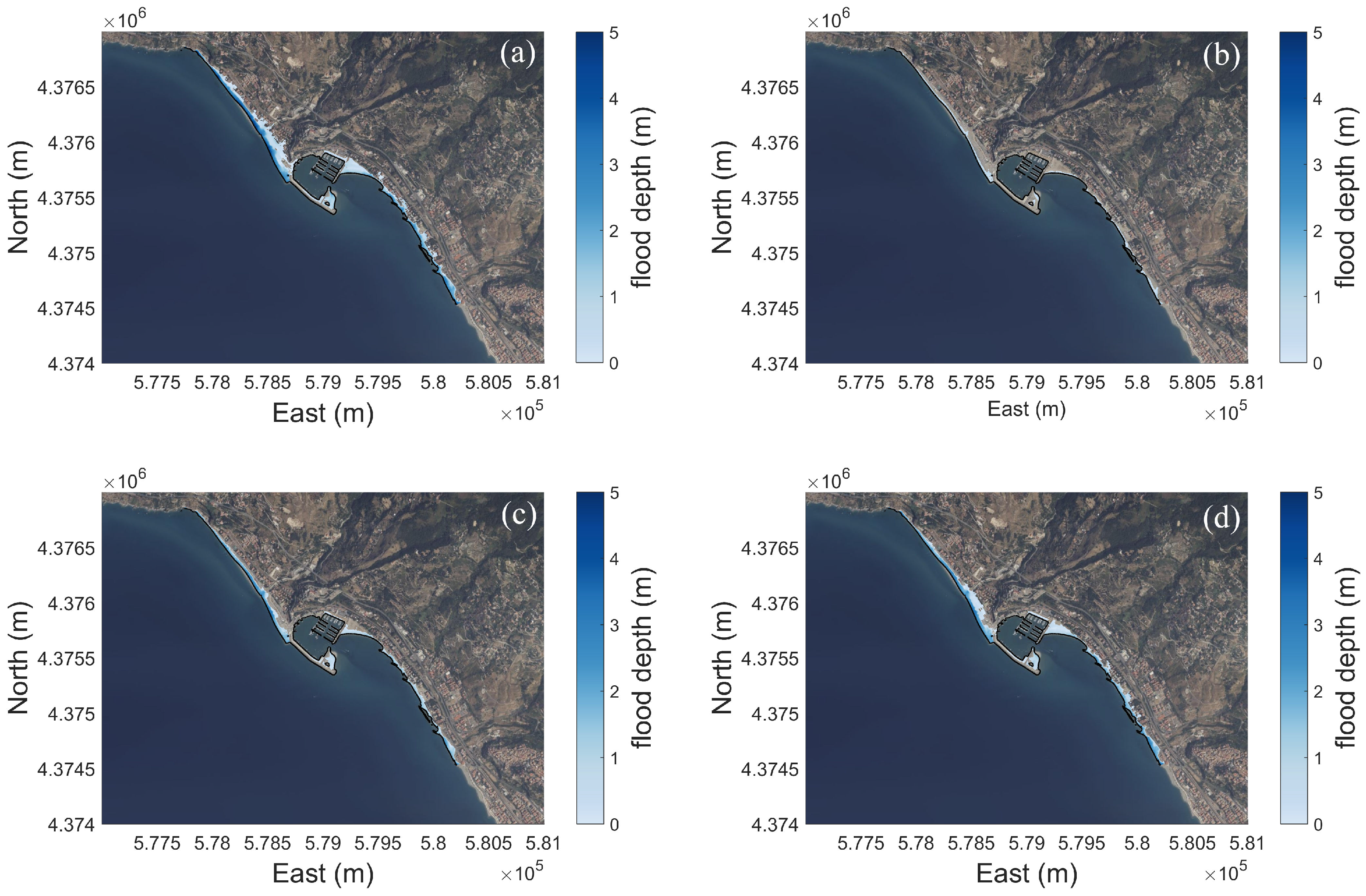
Figure 13, Figure 14 and Figure 15 show the XBeach simulation results in terms of the spatial distribution of maximum flood depths over the emerged coastal area for the design waves with T = 25, 50, and 100 years, respectively, combined with RCP8.5 SLR, and for the different spatial configurations considered (absence of REWEC1, contiguous REWEC1 arrays, REWEC1 with 10 m gaps, and REWEC1 with 20 m gaps). Owing to their limited spatial extent, the inundation maps associated with the P95 of H s , combined with RCP8.5 SLR, were not shown; their effects were instead analyzed in terms of maximum inundated areas, maximum inland water penetration, and wave set-up and run-up in the subsequent analyses. The flooding scenarios, highlighted in Figure 13, Figure 14 and Figure 15, represent the most unfavorable conditions, i.e., the maximum flood depths reached at each computational cell during the simulation time. Accordingly, inundated areas and inland water penetration distances refer to their maximum spatial extent. It should be noted that the background orthophoto used for visualization does not correspond temporally to the shoreline position considered in this study, which is indicated by a black line and derived from the topo-bathymetric surveys carried out by the Department of Biology, Ecology and Earth Sciences of the University of Calabria (e.g., [27]). Overall, the simulation results exhibit a spatial variability that is strongly dependent on the emerged coastal topography and on the presence of coastal structures and civil infrastructures. North of the port, the coast is characterized by a wide and gently sloping beach that gradually narrows landward. This sector experiences the largest flooding extent along the study area, with inland water penetration strongly influenced by the spatial arrangement of civil infrastructures. South of the port, inundated areas are generally smaller due to the presence of some rubble-mound breakwaters, a narrower beach, and a complex backshore topography. With reference to the meteo-marine forcing conditions shown (design waves combined with RCP8.5 SLR), slightly more severe flooding conditions are associated with the design wave with T = 100 years in almost all configurations. Compared to the configuration without REWEC1, which exhibits the largest inundated areas, water penetration distances, and flood depths (Figure 13a, Figure 14a and Figure 15a), the presence of REWEC1 devices results in a clear reduction in these quantities due to wave energy dissipation in their lee. In particular, contiguous REWEC1 arrays produce the most significant reduction in inundated areas (Figure 13b, Figure 14b and Figure 15b), followed by configurations with 10 m gaps (Figure 13c, Figure 14c and Figure 15c) and 20 m gaps (Figure 13d, Figure 14d and Figure 15d).
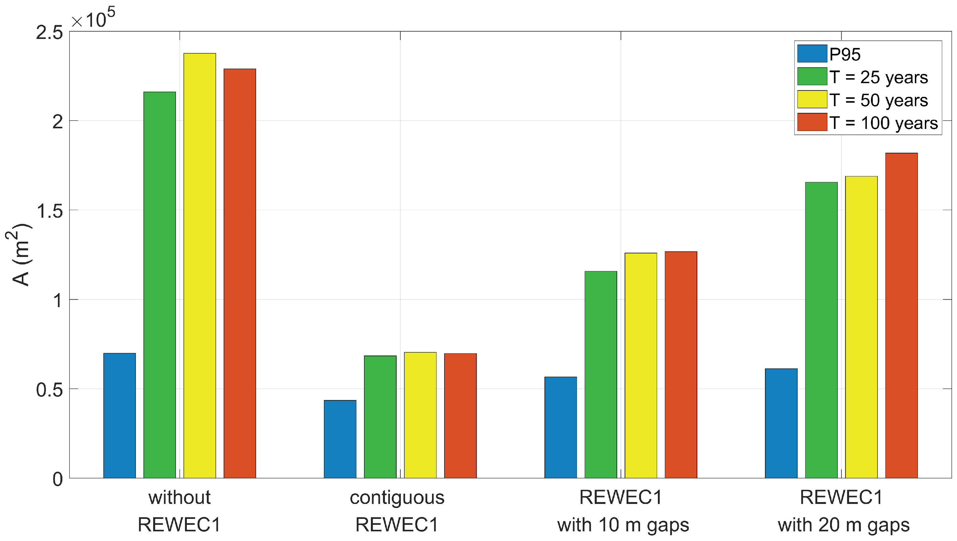
For all spatial configurations, Figure 16 shows the maximum flooded areas A along the entire coast, distinguishing between cases using the P95 of H s and those using design waves with T = 25, 50, and 100 years, all combined with RCP8.5 SLR. Except for the cases without REWEC1 and with contiguous REWEC1, the highest values of A are associated with the design wave with T = 100 years. Progressive reductions in A occur with the inclusion of REWEC1 devices, from the configuration with 20 m gaps to the contiguous configuration. Moreover, the reduction in A associated with the selected design wave conditions is essentially similar across all REWEC1 configurations and larger than that associated with P95 of H s . This different behavior is related to the more dissipative nature of the REWEC1 in no-air conditions compared to the device operating in fixed-air conditions. It is worth noting that the relatively large extent of flooded areas is associated with the extreme value of the adopted SLR.
A quantitative assessment of the percentage reduction in maximum inundated area due to the presence of REWEC1 devices operating in no-air and fixed-air modes under all meteo-marine forcing conditions is reported in Table 1. The table defines the relative variation Δ A / A N , where Δ A is the difference between the maximum inundated area in the absence and presence of REWEC1, and A N is the maximum inundated area without REWEC1. The results indicate that the percentage reductions in maximum inundated area are more pronounced under design wave conditions than when the P95 of H s is used as wave forcing, highlighting the effectiveness of REWEC1 in mitigating coastal flooding during extreme wave events. For all the design wave conditions considered, an average reduction of approximately 69% is observed for contiguous REWEC1 arrays, about 46% for the configuration with 10 m gaps, and about 24% for the configuration with 20 m gaps.
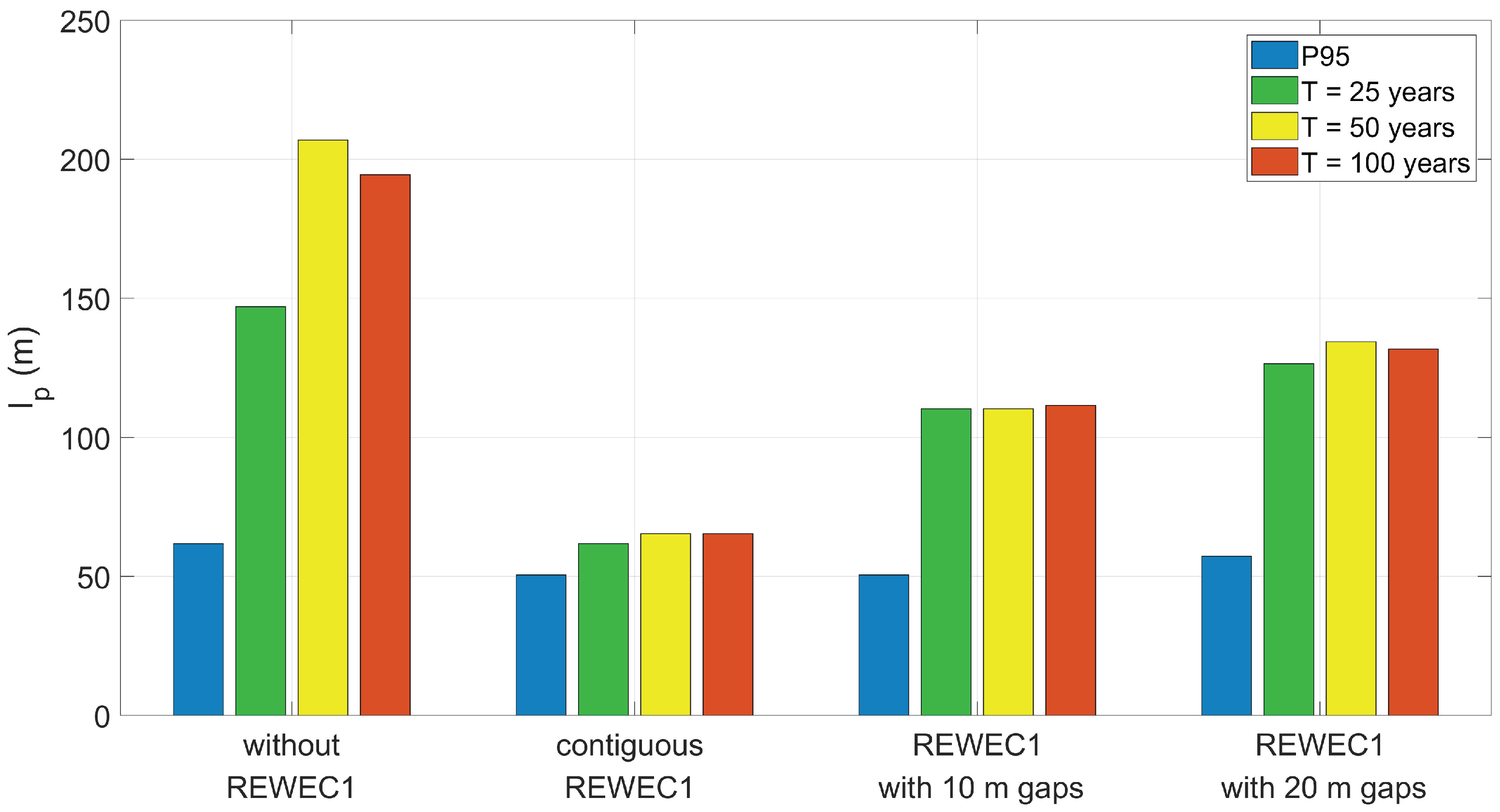
Similarly, Figure 17 presents the maximum inland water penetration lengths l p for the different configurations and the adopted wave conditions (P95 of H s and design waves with T = 25, 50, and 100 years), all combined with RCP8.5 SLR. The values range from maximum values of approximately 200 m in the absence of REWEC1 to values slightly above 50 m for the contiguous configuration, exhibiting trends comparable to those observed for the maximum inundated areas under the different wave conditions. Also in this case, SLR appears to play a relevant role in the assessment of l p .
Table 2 reports the relative reduction Δ l p / l p N , where Δ l p is the difference between the maximum penetration length in the absence and presence of REWEC1, and l p N is the maximum penetration length without REWEC1. The results highlight a progressive attenuation of inland water penetration from the configuration with 20 m gaps to that with contiguous devices. The reduction percentages are quite comparable to those obtained for inundated areas (with mean variations of a few percentage points), being more pronounced under design wave conditions.
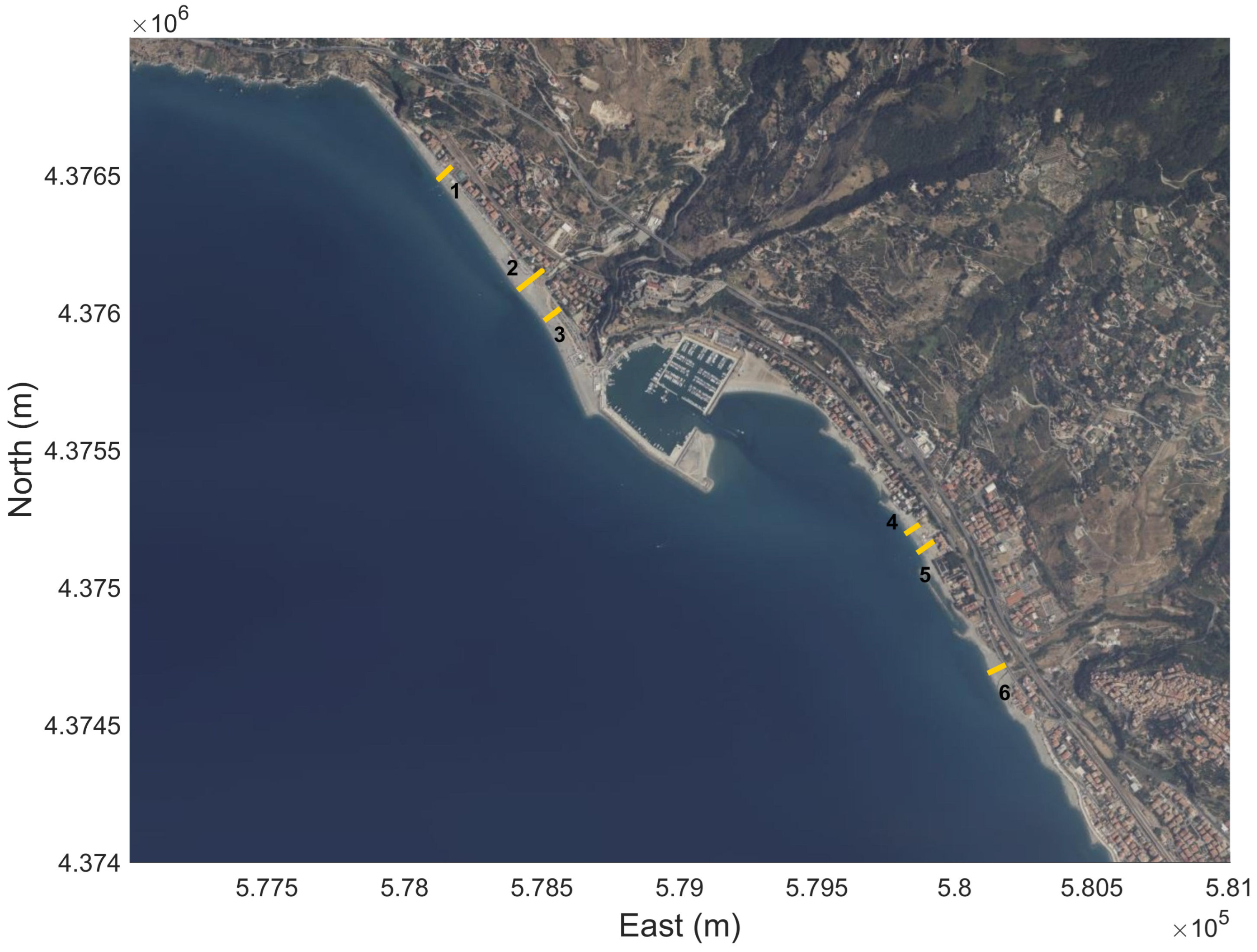
A local-scale quantification of the flooding mitigation effects induced by the presence of REWEC1 devices operating in no-air and fixed-air modes was finally carried out by analyzing wave set-up and run-up. To this end, a set of numerical gauges was placed along selected coastal transects using the XBeach model. Three transects were selected North of the port of Cetraro (transects 1, 2, and 3) and three South of the port (transects 4, 5, and 6), as shown in Figure 18.
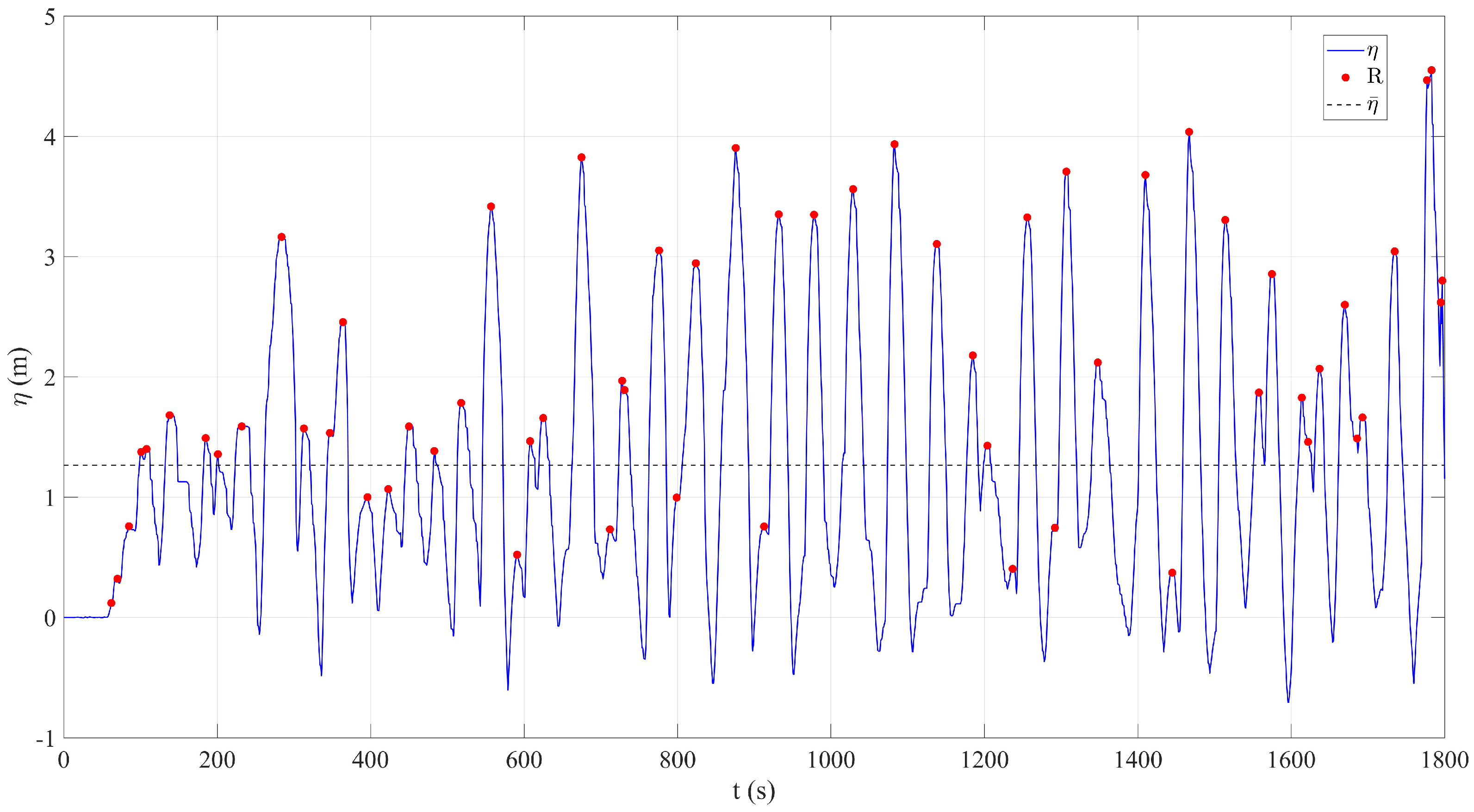
The time series of water levels η extracted at the numerical gauges from XBeach simulations were first corrected by removing the constant SLR contribution. The corrected time series were then preliminarily processed to remove high-frequency noise and isolated numerical spikes. A Hampel filter was applied, which detects outliers within a moving window based on deviations from the local median expressed as multiples of the median absolute deviation [52]. The filtered time series were then used to compute the wave setup η ¯ as the temporal mean. To identify physically meaningful positive maxima corresponding to individual run-up events R, three criteria were adopted. The first criterion concerns the minimum prominence, set equal to 0.01   σ η , where σ η is the standard deviation of the filtered time series [53]. The second criterion imposes a minimum duration of run-up events equal to 0.1   T p [54], where T p is obtained from spectral analysis of the filtered signal. The third criterion requires a minimum temporal separation between consecutive run-up events equal to 0.4   T p [55]. An example of a water level time window for numerical gauge 1, including the identification of individual run-up events and the set-up level, is shown in Figure 19.
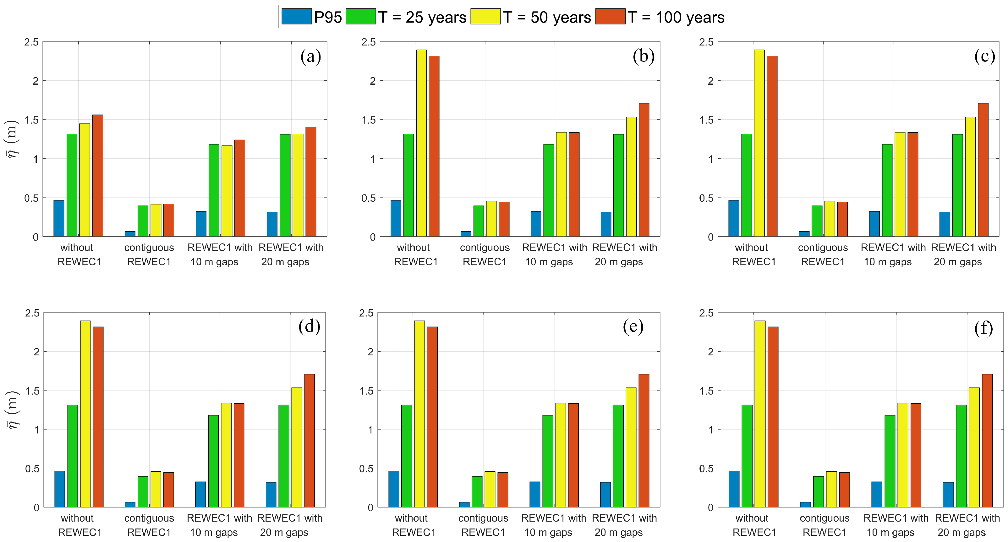
For the different spatial configurations, the computed set-up values η ¯ at the selected numerical gauges are reported in Figure 20, referring to the P95 of H s and the design waves with T = 25, 50, and 100 years. The results exhibit variability depending on the local coastal morphology and on the characteristics of the incident wave field. In general, for all gauges, a progressive reduction in wave set-up is observed due to the presence of REWEC1 devices, from configurations with 20 m gaps to those with contiguous arrays, in agreement with the results obtained for maximum inundated areas and inland water penetrations. The difference in magnitude between the results obtained from the P95 of H s and the different design waves is larger than in the cases of inundated areas and inland water penetration, as SLR was not considered in this analysis.
Table 3 reports the percentage reduction of wave set-up due to the presence of REWEC1 devices, expressed as the relative variation Δ η ¯ / η ¯ N , where Δ η ¯ is the difference between set-up values in the absence and presence of REWEC1, and η ¯ N is the set-up without REWEC1. The reductions exhibit spatial variability among numerical gauges due to the combined effects of local morphology and wave incidence. For contiguous REWEC1 arrays and for the configuration with 10 m gaps, the average set-up reduction is similar across all wave conditions, with mean values of 80.4% and 39.3%, respectively. For the configuration with 20 m gaps, the wave condition associated with the P95 of H s leads to a mean set-up reduction of 31.6%, whereas the design wave conditions result in a mean set-up reduction of 18.4%.
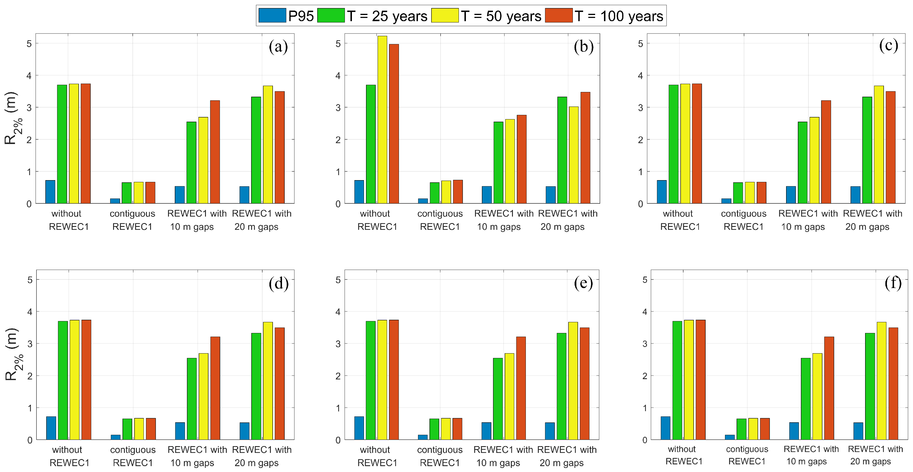
From the individual run-up events R recorded at each numerical gauge, the run-up exceeded by 2% of the events, R 2 % , corresponding to the 98th percentile of the R distribution, was computed. This parameter is statistically robust and widely used in engineering applications. Figure 21 shows the values of R 2 % at the selected gauges for the different spatial configurations, for the P95 of H s and for the design waves with T = 25, 50, and 100 years. The results for R 2 % further confirm the effectiveness of the REWEC1 devices in reducing the main hydrodynamic processes affecting the emerged coast.
Table 4 summarizes the percentage reductions of R 2 % induced by the presence of REWEC1 devices, expressed as the relative variation Δ R 2 % / R 2 % N , where Δ R 2 % is the difference between R 2 % values in the absence and presence of REWEC1, and R 2 % N is the run-up value without REWEC1. As for wave set-up, the reduction percentages are influenced by local coastal morphology and wave incidence. Overall, the average reduction of R 2 % is fairly similar of that observed for η ¯ (see Table 3) for all wave conditions and REWEC1 configurations. The differences in mean reduction between R 2 % and η ¯ are less than 2%.

5.4. Uncertainty Analysis

An uncertainty analysis was conducted to evaluate the sensitivity of XBeach simulations to variations in the transmission coefficient C T of the REWEC1 devices. In the SWAN simulations, the C T values of REWEC1 for the selected spatial arrangements (contiguous, 10 m gaps, and 20 m gaps), obtained by the undisturbed wave field at a water depth of 10 m, were systematically varied by ± 15 % to account for potential deviations arising from modeling assumptions, operational conditions, or inherent variability. Notably, C T is a numerically derived parameter according to Filianoti and Piscopo [21] and represents the principal hydraulic parameter for assessing the effectiveness of REWEC1 in reducing coastal flooding. In this analysis, the reflection coefficients C R were kept fixed with respect to the reference values, as their values for the REWEC1 are consistently very low and their contribution to coastal flooding processes is negligible compared to transmission-driven effects.
The analysis focused on the worst-case scenario, corresponding to the design wave with T = 100 years combined with RCP8.5 SLR. In this context, the REWEC1 units operated in no-air mode. The evaluation metrics were the maximum inundated areas and the maximum inland water penetration lengths. Comparing simulations with perturbed C T values to the previous baseline results allowed for the quantification of uncertainty and the assessment of model robustness. This approach aligns with previous studies on uncertainty and sensitivity analysis in coastal hydrodynamic modeling (e.g., [56]), underscoring the importance of accounting for parameter variability when evaluating extreme events.
Based on the variability of the wave parameters at a water depth of 10 m for the selected design wave, C T ranges between 0.171 and 0.174 when the coefficient is reduced by 15%, and between 0.231 and 0.236 when it is increased by 15%. The disturbed wave field behind the REWEC1 at d = 7 m, obtained from SWAN simulations for different spatial configurations, was used as input, together with RCP8.5 SLR, for the subsequent XBeach simulations.
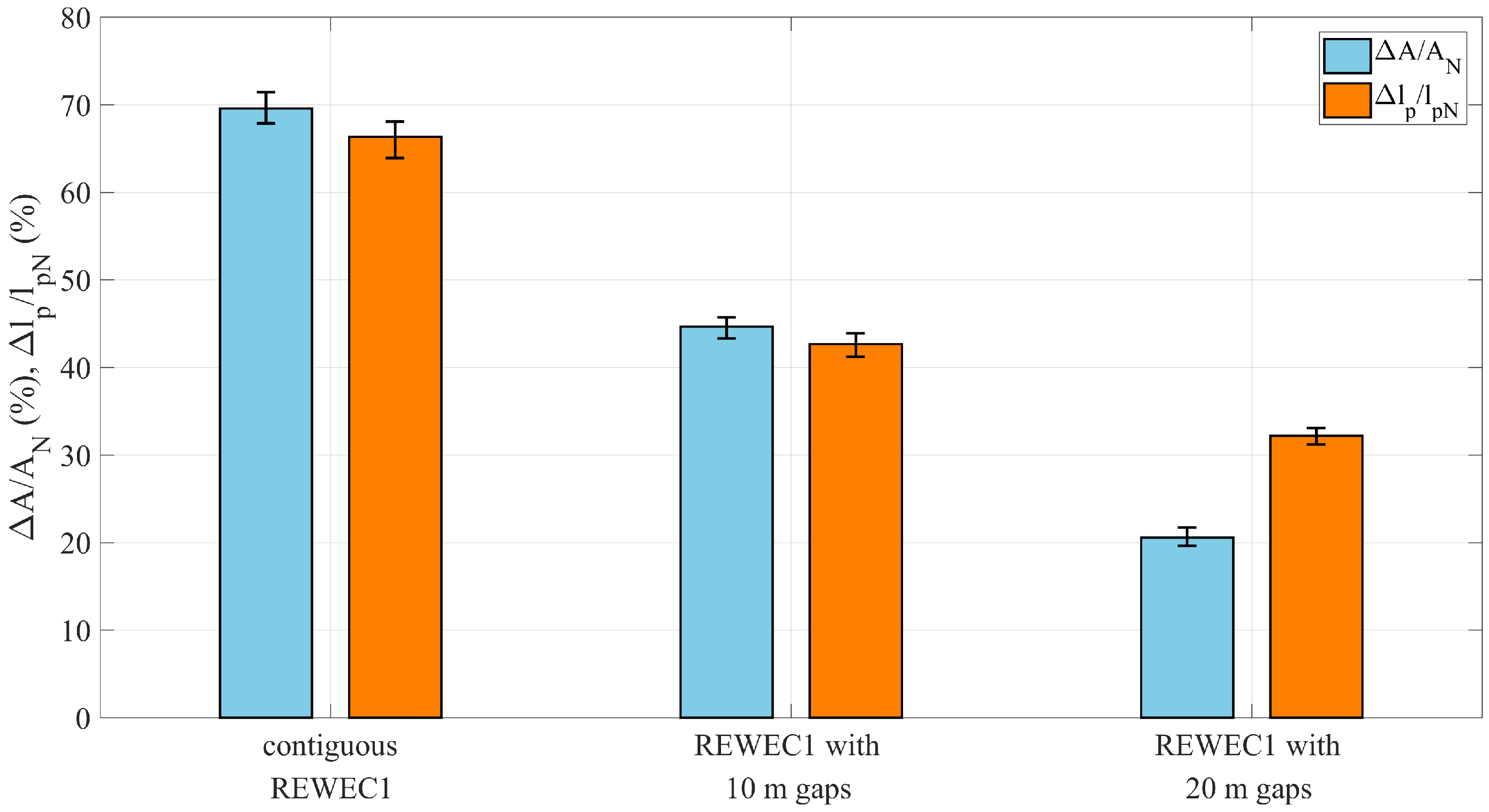
To analyze the sensitivity of coastal flooding to variations in the wave transmission coefficient C T of the REWEC1 devices, two indicators were selected: the maximum inundated area and the maximum inland water penetration length. For the adopted spatial configurations (contiguous arrays, arrays with 10 m gaps, and arrays with 20 m gaps), Figure 22 shows the relative reductions of flooding indicators Δ A / A N and Δ l p / l p N obtained using the reference C T values and those derived by perturbing this parameter by ± 15 % . Error bars are used to visualize the resulting variability, providing a quantitative representation of the potential range of outcomes under the selected extreme meteo-marine condition. The variability in Δ A / A N and Δ l p / l p N is generally small across all configurations, decreasing from approximately 4% for contiguous REWEC1 arrays to about 2% for arrays with 20 m gaps. Lower reductions in flooding indicators are observed for higher C T values, while higher reductions correspond to lower C T values. A slightly larger variability is noted for cases with higher C T values, particularly in the contiguous configuration, highlighting the increased sensitivity of closely spaced arrays to changes in hydraulic performance. Overall, these results demonstrate that the selected ± 15 % variation in C T induces only minor changes in the predicted inundation patterns, regardless of the spatial configuration. This confirms the robustness and consistency of the trends reported in Section 5.3, and supports the reliability of the REWEC1 performance assessment even under moderate uncertainties in the transmission coefficient.

5.5. Comparison with Rubble-Mound Breakwaters

In this Section, a comparison between REWEC1 and traditional submerged rubble-mound breakwaters in reducing coastal flooding was performed. The analysis considered the most extreme meteo-marine condition, i.e., the design wave with T = 100 years combined with RCP8.5 SLR, across all spatial configurations (contiguous barriers, barriers with 10 m gaps, and barriers with 20 m gaps) operating in no-air mode.
The submerged rubble-mound breakwaters were placed at the same water depth ( d = 10 m) and with the same height and length as the REWEC1 devices. They were composed of natural stones with a canonical seaward slope (tan( α ) = 0.5) and an armour layer with a mean diameter of 2 m, ensuring stability under the applied wave forcing. To provide a consistent comparison, the hydraulic behaviour of the submerged rubble-mound breakwaters was modelled using transmission C T and reflection C R coefficients that depend solely on the incident wave conditions. Similar to REWEC1, SLR effects were not explicitly included in the coefficient formulation but were incorporated as a shift in the mean water level for the coastal flooding simulations.
The hydraulic characteristics adopted in SWAN simulations, in terms of C T and C R , were derived from various experimental-based formulas for low-crested rubble-mound breakwaters. For C T , the semi-empirical equations developed by d’Angremond [57], Seabrook and Hall [58], and Briganti et al. [59] were applied, which are valid within the range of the considered wave and geometrical conditions. Considering the variability of the incident wave parameters at d = 10 m, the resulting C T values obtained from the aforementioned formulas were averaged, yielding values between 0.364 and 0.397 depending on the specific location of the rubble mound breakwater and the local wave conditions. Similarly, C R was derived by averaging the results from semi-empirical formulas by Seelig and Ahrens [60], Ahrens [61], and Zanuttigh and van der Meer [62], resulting in values ranging from 0.260 to 0.278.
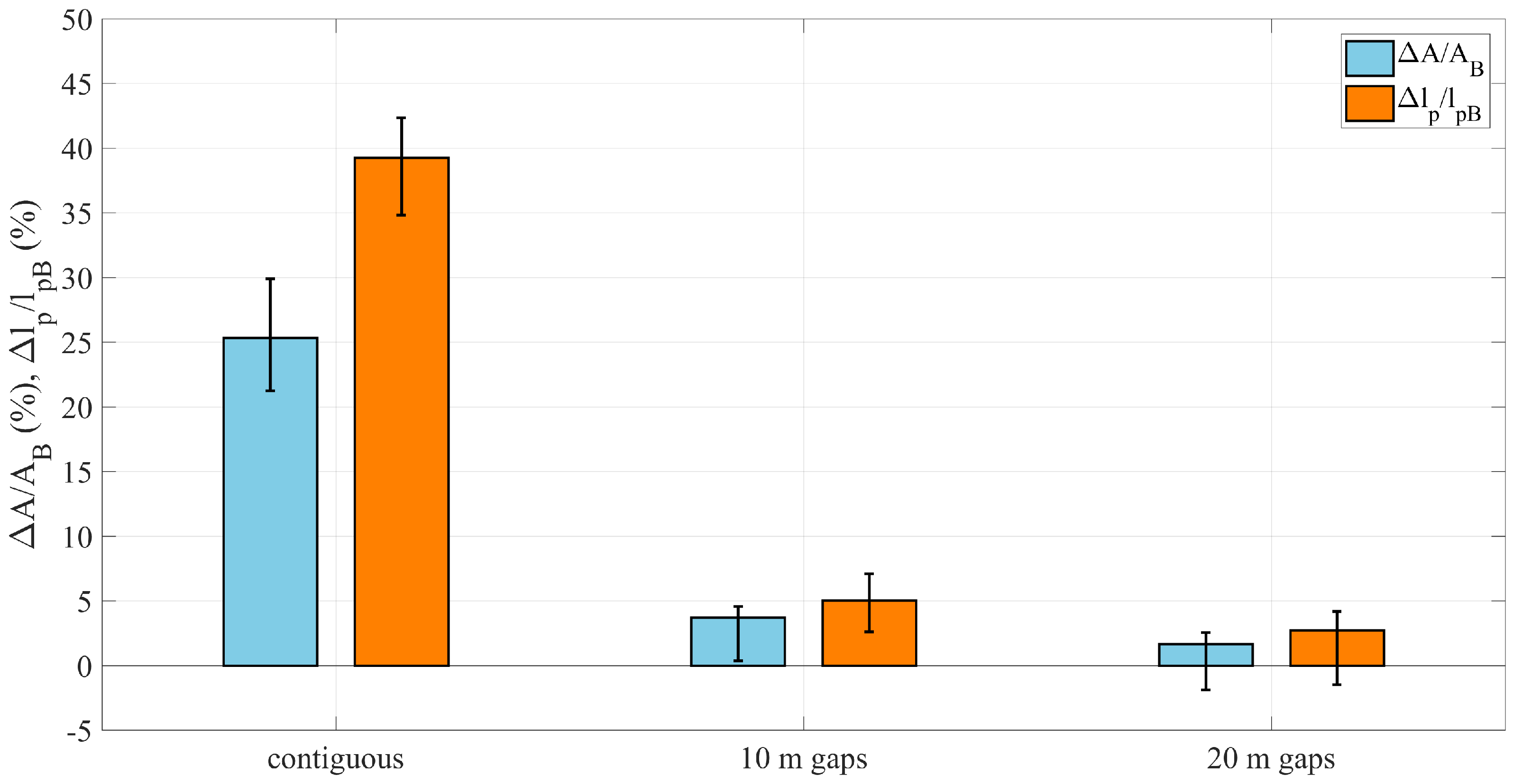
The wave field behind the rubble-mound breakwaters for all spatial configurations at a water depth of 7 m, induced by the T = 100 year design wave and obtained from SWAN, was used as input for the XBeach simulations of coastal flooding, also accounting for RCP8.5 SLR. The resulting maximum flooded areas and maximum inland water penetration lengths were then compared with those obtained for the REWEC1 devices. In the comparison between REWEC1 and conventional rubble-mound breakwaters, the evaluation of flooding indicators for REWEC1 explicitly accounts for the uncertainty associated with a ±15% variation in the transmission coefficient C T . This level of uncertainty is not considered for rubble-mound breakwaters, whose hydraulic performance is derived from well-established empirical relationships based on extensive experimental studies. The relative reductions in the flooding indicators Δ A / A B and Δ l p / l p B were evaluated by comparing REWEC1 and rubble-mound breakwaters for different spatial configurations. The indicators were computed by defining Δ A and Δ l p as the differences between the maximum inundated area and maximum inland water penetration length in the presence of rubble-mound breakwaters and those obtained with REWEC1, respectively, while A B and l p B denote the corresponding values associated with the rubble-mound breakwaters. This formulation allows a direct assessment of the relative performance of REWEC1 in reducing coastal flooding with respect to conventional submerged breakwaters. The resulting relative reductions are shown in Figure 23. For the contiguous arrangement, consistently positive values of Δ A / A B and, in particular, of Δ l p / l p B are observed, indicating a superior performance of REWEC1 units in mitigating coastal flooding with respect to rubble-mound breakwaters. Conversely, for the configurations with 10 m and 20 m gaps, the values of Δ A / A B and Δ l p / l p B are small and, in some cases, negative, suggesting that the flooding reduction capability of REWEC1 is comparable to that of conventional rubble-mound breakwaters when spatial discontinuities are introduced.


6. Conclusions

This study has shown that REWEC1 devices, whether operating in fixed-air mode (active barrier) or no-air mode (behaving as conventional submerged breakwaters), have a significant effect in terms of reducing coastal flooding and mitigating the associated risk. The magnitude of this reduction is a function of the spatial arrangement adopted for these devices in the coastal protection.
The numerical results were obtained using the SWAN and XBeach models for the Cetraro coast in Southern Italy. The meteo-marine forcing considered the P95 of H s as the recurrent wave conditions for REWEC1 operating in fixed-air mode, and the design waves with T = 25, 50, and 100 years for REWEC1 operating in no-air mode, all combined with the most severe future SLR scenario corresponding to the RCP8.5 projection for the year 2100. In terms of the analyzed indicators (maximum flooded areas, maximum inland penetration lengths, wave set-up, and 2% wave run-up), REWEC1 barriers induce an overall reduction with respect to undisturbed conditions, with magnitudes that depend on the operational mode of the devices (no-air or fixed-air). Specifically, average reductions exceeding 70% and 50% were observed for the contiguous configuration operating in no-air and fixed-air mode, respectively. These reductions decrease when the devices are arranged with gaps, with mean values of about 40% and less than 30% for gaps of 10 m in no-air and fixed-air mode, respectively, and around 20% for gaps of 20 m under both operational conditions. This behavior is consistent with the more dissipative response of the REWEC1 in no-air mode compared with fixed-air mode during wave–structure interaction processes. An uncertainty analysis was also carried out by perturbing the transmission coefficient, identified as the most influential hydraulic parameter for modeling REWEC1 in coastal flooding applications, within a ±15% range. Under the extreme scenario defined by a 100-year design wave combined with SLR, the results show that, despite this variability, REWEC1 units still provide a substantial reduction in coastal flooding compared to undisturbed conditions. The comparison between REWEC1 devices and conventional submerged rubble-mound breakwaters further indicates that, under the same extreme scenario adopted for the uncertainty analysis, REWEC1 leads to smaller inundated areas and reduced inland water penetration only when a contiguous configuration is employed. When spatial discontinuities between the barriers are introduced, the two solutions exhibit comparable performance in terms of coastal flooding mitigation.
Importantly, under less extreme wave conditions, REWEC1 can operate as wave energy converters, producing electricity while continuing to provide an acceptable performance for coastal protection against flooding. In this context, their dual functionality, as both renewable energy generators and effective coastal defense structures, makes them a highly valuable option for sustainable coastal management.
Future research could include laboratory experiments to validate the numerical parameters used to characterize the hydraulic behaviour of REWEC1, i.e., the transmission and reflection coefficients. Additionally, a detailed investigation of the morphodynamic effects induced by REWEC1 in different spatial configurations is recommended, as local bed changes could modify the effectiveness of the devices in reducing coastal flooding.

Author Contributions

Conceptualization, F.A. and P.G.F.F.; methodology, F.A.; software, F.A. and G.T.; formal analysis, F.A. and G.T.; resources, F.A. and G.T.; writing—original draft preparation, F.A.; supervision, P.G.F.F.; funding acquisition, F.A. All authors have read and agreed to the published version of the manuscript.

Funding

This work was funded by the Italian Ministry of Research (MIUR) grant number P20224CY2L under the research project ”SMART—Sea wave energy converters and MARine Tidal turbines”.

Data Availability Statement

The data presented in this study are available on request from the corresponding author due to restrictions related to an ongoing research project and institutional agreements.

Acknowledgments

During the preparation of this manuscript, the authors used ChatGPT (version 5.2) for language editing and readability improvement. The authors have reviewed and edited the output and take full responsibility for the content of this publication.

Conflicts of Interest

The authors declare no conflicts of interest.

References

  1. Vitousek, S.; Barnard, P.L.; Fletcher, C.H.; Frazer, N.; Erikson, L.; Storlazzi, C.D. Doubling of coastal flooding frequency within decades due to sea-level rise. Sci. Rep. 2017, 7, 1399. [Google Scholar] [CrossRef] [Scilit] [PubMed]
  2. Lawyer, C.; Li, A.; Goharian, E. A Review of Climate Adaptation Impacts and Strategies in Coastal Communities: From Agent-Based Modeling towards a System of Systems Approach. Water 2023, 15, 2635. [Google Scholar] [CrossRef] [Scilit]
  3. McInnes, K.L.; Hubbert, G.D.; Abbs, D.J.; Oliver, S.E. A numerical modelling study of coastal flooding. Meteorol. Atmos. Phys. 2002, 80, 217–233. [Google Scholar] [CrossRef] [Scilit]
  4. Narendr, A.; Aithal, B.H.; Das, S. A data-driven framework for enhancing coastal flood resilience in resource-crunched developing nations. Geomat. Nat. Hazards Risk 2024, 15, 2396892. [Google Scholar] [CrossRef] [Scilit]
  5. Baart, F.; de Boer, G.; Pronk, M.; van Koningsveld, M.; Muis, S. A semantic notation for comparing global high-resolution coastal flooding studies. Front. Earth Sci. 2024, 12, 1465040. [Google Scholar] [CrossRef] [Scilit]
  6. Ahmadian, A.S. Numerical Models for Submerged Breakwaters: Coastal Hydrodynamics and Morphodynamics; Butterworth-Heinemann: Amsterdam, The Netherlands, 2006; pp. 1–362. [Google Scholar]
  7. Marino, M.; Baptist, M.J.; Alkharoubi, A.I.K.; Nasca, S.; Cavallaro, L.; Foti, E.; Musumeci, R.E. Nature-based Solutions as Building Blocks for coastal flood risk reduction: A model-based ecosystem service assessment. Sci. Rep. 2025, 15, 12070. [Google Scholar] [CrossRef] [Scilit]
  8. Park, S.; Sohn, W.; Piao, Y.; Lee, D. Adaptation strategies for future coastal flooding: Performance evaluation of green and grey infrastructure in South Korea. J. Environ. Manag. 2023, 334, 117495. [Google Scholar] [CrossRef] [Scilit]
  9. Boodoo, A.; Wakeyama, T.; Cross, J.S. Wave farms for coastal protection: A systematic review of effectiveness, methodologies, and future directions. Ocean Coast. Manag. 2025, 269, 107807. [Google Scholar] [CrossRef] [Scilit]
  10. Astariz, S.; Iglesias, G. The economics of wave energy: A review. Renew. Sustain. Energy Rev. 2015, 45, 397–408. [Google Scholar] [CrossRef] [Scilit]
  11. Mustapa, M.A.; Yaakob, O.B.; Ahmed, Y.M.; Rheem, C.-K.; Koh, K.K.; Adnan, F.A. Wave energy device and breakwater integration: A review. Renew. Sustain. Energy Rev. 2017, 77, 43–58. [Google Scholar] [CrossRef] [Scilit]
  12. Abanades, J.; Greaves, D.; Iglesias, G. Wave farm impact on the beach profile: A case study. Coast. Eng. 2014, 86, 36–44. [Google Scholar] [CrossRef] [Scilit]
  13. Mendoza, E.S.R.; Zanuttigh, B.; Angelelli, E.; Andersen, T.L.; Martinelli, L.; Nørgaard, J.Q.H.; Ruol, P. Beach response to wave energy converter farms acting as coastal defence. Coast. Eng. 2014, 87, 97–111. [Google Scholar] [CrossRef] [Scilit]
  14. Bergillos, R.J.; López-Ruiz, A.; Medina-López, E.; Moñino, A.; Ortega-Sánchez, M. The role of wave energy converter farms on coastal protection in eroding deltas, Guadalfeo, southern Spain. J. Clean. Prod. 2018, 171, 356–367. [Google Scholar] [CrossRef] [Scilit]
  15. Ozkan, C.; Perez, K.; Mayo, T. The impacts of wave energy conversion on coastal morphodynamics. Sci. Total Environ. 2020, 712, 136424. [Google Scholar] [CrossRef] [Scilit]
  16. Bergillos, R.J.; Rodriguez-Delgado, C.; Iglesias, G. Wave farm impacts on coastal flooding under sea-level rise: A case study in southern Spain. Sci. Total Environ. 2019, 653, 1522–1531. [Google Scholar] [CrossRef] [Scilit]
  17. Bergillos, R.J.; Rodriguez-Delgado, C.; Allen, J.; Iglesias, G. Wave energy converter geometry for coastal flooding mitigation. Sci. Total Environ. 2019, 668, 1232–1241. [Google Scholar] [CrossRef] [Scilit]
  18. Boccotti, P. Gli Impianti REWEC; Bios Ed.: Castrolibero, Italy, 2004; pp. 1–120. [Google Scholar]
  19. Boccotti, P. On a new wave energy absorber. Ocean Eng. 2003, 30, 1191–1200. [Google Scholar] [CrossRef] [Scilit]
  20. Arena, F.; Filianoti, P. A small-scale field experiment on a submerged breakwater for absorbing wave energy. J. Waterw. Port Coast. Ocean Eng. 2007, 133, 161–167. [Google Scholar] [CrossRef] [Scilit]
  21. Filianoti, P.; Piscopo, R. Sea wave energy transmission behind submerged absorber caissons. Ocean Eng. 2015, 93, 107–117. [Google Scholar] [CrossRef] [Scilit]
  22. Filianoti, P.; Gurnari, L.; Torresi, M.; Camporeale, S.M. CFD analysis of the energy conversion process in a fixed oscillating water column (OWC) device with a Wells turbine. Energy Procedia 2018, 148, 1026–1033. [Google Scholar] [CrossRef] [Scilit]
  23. Filianoti, P.; Gurnari, L. The Performance of an “Active” Submerged Breakwater by a CFD Analysis. In Proceedings of the 29th International Ocean and Polar Engineering Conference, Honolulu, HI, USA, 16–21 June 2019. ISOPE-I-19-379. [Google Scholar]
  24. Gurnari, L.; Filianoti, P.; Torresi, M.; Camporeale, S.M. The wave-to-wire energy conversion process for a fixed U-OWC device. Energies 2020, 13, 283. [Google Scholar] [CrossRef] [Scilit]
  25. Booij, N.; Ris, R.C.; Holthuijsen, L.H. A third-generation wave model for coastal regions: 1. Model description and validation. J. Geophys. Res. 1999, 104, 7649–7666. [Google Scholar] [CrossRef] [Scilit]
  26. Roelvink, D.; Reniers, A.; van Dongeren, A.; van Thiel de Vries, J.; McCall, R.; Lescinski, J. Modeling storm impacts on beaches, dunes and barrier islands. Coast Eng. 2009, 56, 1133–1152. [Google Scholar] [CrossRef] [Scilit]
  27. Cianflone, G.; Imbrogno, G.; Flaubert Nguebiapssi Kembeu, F.N.; Penna, N.; Ferraro, D.; Cirillo, D.; Ietto, F.; Dominici, R. By-pass sediment system to replace longshore current in harbour areas. Ital. J. Eng. Geol. Environ. 2024, 1, 57–67. [Google Scholar]
  28. Caloiero, T.; Aristodemo, F.; Algieri Ferraro, D. Trend analysis of significant wave height and energy period in southern Italy. Theor. Appl. Climatol. 2019, 138, 917–930. [Google Scholar] [CrossRef] [Scilit]
  29. Aristodemo, F.; Algieri Ferraro, D. Feasibility of WEC installations for domestic and public electrical supplies: A case study off the Calabrian coast. Renew. Energy 2018, 121, 261–285. [Google Scholar] [CrossRef] [Scilit]
  30. Foti, G.; Barbaro, G.; Besio, G.; Barillà, G.C.; Mancuso, P.; Puntorieri, P. Wave climate along Calabrian coasts. Climate 2022, 10, 80. [Google Scholar] [CrossRef] [Scilit]
  31. Soulsby, R.L. Dynamics of Marine Sands; Thomas Telford Publications: London, UK, 1997; pp. 1–249. [Google Scholar]
  32. Van Rijn, L.C. Sediment transport, part III: Bed forms and alluvial roughness. J. Hydr. Eng. 1985, 110, 1733–1754. [Google Scholar] [CrossRef] [Scilit]
  33. McCall, R.T.; Van Thiel de Vries, J.S.M.; Plant, N.G.; Van Dongeren, A.R.; Roelvink, J.A.; Thompson, D.M.; Reniers, A.J.H.M. Two-dimensional time dependent hurricane overwash and erosion modeling at Santa Rosa Island. Coast Eng. 2010, 57, 668–683. [Google Scholar] [CrossRef] [Scilit]
  34. Vousdoukas, M.I.; Ferreira, O.; Almeida, L.P.; Pacheco, A. Toward reliable storm-hazard forecasts: XBeach calibration and its potential application in an operational early-warning system. Ocean Dyn. 2012, 62, 1001–1015. [Google Scholar] [CrossRef] [Scilit]
  35. Saponieri, A.; Di Risio, M.; Pasquali, D.; Valentini, N.; Aristodemo, F.; Tripepi, G.; Celli, D.; Streicher, M.; Damiani, L. Beach profile evolution in front of storm seawalls: A physical and numerical study. In Proceedings of the 36th International Conference on Coastal Engineering, Baltimore, MD, USA, 30 July–3 August 2018; p. 70. [Google Scholar]
  36. Mentaschi, L.; Besio, G.; Cassola, F.; Mazzino, A. Performance evaluation of Wavewatch III in the Mediterranean Sea. Ocean Model. 2015, 90, 82–94. [Google Scholar] [CrossRef] [Scilit]
  37. Lira-Loarca, A.; Cobos, M.; Besio, G.; Baquerizo, A. Projected wave climate temporal variability due to climate change. Stoch. Environ. Res. Risk Assess. 2021, 302, 117492. [Google Scholar]
  38. Aristodemo, F.; Lira-Loarca, A.; Besio, G.; Caloiero, T. Detection and quantification of wave trends in the Mediterranean basin. Dyn. Atmos. Oceans 2024, 105, 101413. [Google Scholar] [CrossRef] [Scilit]
  39. Piscopia, R.; Inghilesi, R.; Panizzo, A.; Corsini, S.; Franco, L. Analysis of 12-year wave measurements by the Italian wave Network. In Proceedings of the 28st International Conference on Coastal Engineering, Cardiff, Wales, 7–12 July 2002; pp. 121–133. [Google Scholar]
  40. Goda, Y. On the methodology of selecting design wave height. In Proceedings of the 21st International Conference on Coastal Engineering, Torremolinos, Spain, 20–25 June 1988; pp. 899–913. [Google Scholar]
  41. Katalinić, M.; Parunov, J. Comprehensive Wind and Wave Statistics and Extreme Values for Design and Analysis of Marine Structures in the Adriatic Sea. J. Mar. Sci. Eng. 2021, 9, 522. [Google Scholar] [CrossRef] [Scilit]
  42. Soukissian, T.H.; Karathanasi, F.E. Joint Modelling of Wave Energy Flux and Wave Direction. Processes 2021, 9, 460. [Google Scholar] [CrossRef] [Scilit]
  43. Forristall, G.Z. Wave crest distributions: Observations and second-order theory. J. Phys. Oceanogr. 2000, 30, 1931–1943. [Google Scholar] [CrossRef] [Scilit]
  44. Golden Software LLC. Surfer: Contouring, Gridding, and Surface Mapping Software; Golden Software LLC.: Golden, CO, USA, 2018. [Google Scholar]
  45. Haigh, I.; Nicholls, R.; Wells, N. Assessing changes in extreme sea levels: Application to the English Channel, 1900–2006. Cont. Shelf Res. 2010, 30, 1042–1055. [Google Scholar] [CrossRef] [Scilit]
  46. Vousdoukas, M.I.; Mentaschi, L.; Voukouvalas, E.; Verlaan, M.; Jevrejeva, S.; Jackson, L.P.; Feyen, L. Global probabilistic projections of extreme sea levels show intensification of coastal flood hazard. Nat. Commun. 2018, 9, 2360. [Google Scholar] [CrossRef] [Scilit]
  47. Holthuijsen, L.H.; Herman, A.; Booij, N. Phase-decoupled refraction-diffraction for spectral wave models. Coast Eng. 2003, 49, 291–305. [Google Scholar] [CrossRef] [Scilit]
  48. U.S. Army Corps of Engineers (USACE). Coastal Engineering Manual (EM 1110-2-1100); U.S. Army Corps of Engineers (USACE): Washington, DC, USA, 2002. [Google Scholar]
  49. CIRIA; CUR; CETMEF. The Rock Manual: The Use of Rock in Hydraulic Engineering, 2nd ed.; CIRIA: London, UK, 2007. [Google Scholar]
  50. IPCC. Sixth Assessment Report of the Intergovernmental Panel on Climate Change; IPCC: Geneva, Switzerland, 2021. [Google Scholar]
  51. Deltares. Delft3D-RGFGRID User Manual; Generation and Manipulation of Structured and Unstructured Grids, Suitable for Delft3D-FLOW, Delft3D-WAVE or D-Flow Flexible Mesh; Deltares: Delft, The Netherlands, 2025; pp. 1–140. [Google Scholar]
  52. Goring, D.G.; Nikora, V.I. Despiking Acoustic Doppler Velocimeter Data. J. Hydr. Eng. 2002, 128, 117–126. [Google Scholar] [CrossRef] [Scilit]
  53. Holman, R.A. Extreme value statistics for wave run-up on a natural beach. Coast. Eng. 1986, 9, 527–544. [Google Scholar] [CrossRef] [Scilit]
  54. Yeh, H.H.; Ghazali, A.; Marton, I. Experimental study of bore run-up. J. Fluid Mech. 1989, 206, 563–578. [Google Scholar] [CrossRef] [Scilit]
  55. Guza, R.T.; Thornton, E.B. Swash oscillations on a natural beach. J. Geophys. Res. Oceans 1982, 87, 483–491. [Google Scholar] [CrossRef] [Scilit]
  56. de Moel, H.; Asselman, N.E.M.; Aerts, J.C.J.H. Uncertainty and sensitivity analysis of coastal flood damage estimates in the west of the Netherlands. Nat. Hazards Earth Syst. Sci. 2012, 12, 1045–1058. [Google Scholar] [CrossRef] [Scilit]
  57. d’Angremond, K.; van der Meer, J.W.; De Jong, R. Wave transmission at low-crested structures. In Proceedings of the 25st International Conference on Coastal Engineering, Orlando, FL, USA, 2–6 September 1996; pp. 2418–2427. [Google Scholar]
  58. Seabrook, S.R.; Hall, K.R. Wave transmission at submerged rubblemound breakwaters. In Proceedings of the 26st International Conference on Coastal Engineering, Copenhagen, Denmark, 22–26 June 1998; pp. 2000–2013. [Google Scholar]
  59. Briganti, R.; van der Meer, J.W.; Buccino, M.; Calabrese, M. Wave transmission behind low-crested structures. In Proceedings of the Coastal Structures, Portland, OR, USA, 26–30 August 2003; pp. 580–592. [Google Scholar]
  60. Seelig, W.N.; Ahrens, J.P. Estimation of Wave Reflection and Energy Dissipation Coefficient for Beaches, Revetments and Breakwaters; Technical Paper 81-1 U.S. Army Corps of Engineers; Coastal Engineering Research Center: Fort Belvoir, VA, USA, 1981; pp. 1–40. [Google Scholar]
  61. Ahrens, J.P. Characteristics of Reef Breakwaters; Technical Report CERC-87-17 Army Corps of Engineers; Coastal Engineering Research Center: Vicksburg, MI, USA, 1987; pp. 1–66. [Google Scholar]
  62. Zanuttigh, B.; van der Meer, J.W. Wave reflection from coastal structures in design conditions. Coast. Eng. 2008, 55, 771–779. [Google Scholar] [CrossRef] [Scilit]
Figure 1. Schematic configuration of a REWEC1 device. (a) fixed-air operation mode; (b) no-air operation mode.
Water 18 00524 g001
Figure 2. (a) Trends of the absorption C A , dissipation C L , and transmission C T coefficients versus significant wave height H s for a REWEC1 device in fixed-air operation mode; (b) Trends of the dissipation C L and transmission C T coefficients versus significant wave height H s for a REWEC1 device in no-air operation mode.
Water 18 00524 g002
Figure 3. Map of Italy with the position of the Calabria region and the Cetraro site.
Water 18 00524 g003
Figure 4. Percentage occurrence of wave events within the Cetraro cross-shore sector, classified by 10° directional bins and by different significant wave height intervals.
Water 18 00524 g004
Figure 5. Trend of the averaged values of H s and T p (black dots) and regression curve in power-law form (magenta curve) for the 250°–280° directional sector.
Water 18 00524 g005
Figure 6. Spatial variation of significant wave height H s along nodes located near the 10 m water depth. (a) P95 of H s ; (b) design wave with T = 25 years; (c) design wave with T = 50 years; (d) design wave with T = 100 years.
Water 18 00524 g006
Figure 7. Detail of the spatial configuration of the REWEC1 devices, including the local bathymetry. (a) contiguous REWEC1; (b) REWEC1 with 10 m gaps; (c) REWEC1 with 20 m gaps.
Water 18 00524 g007
Figure 8. Spatial distribution of significant wave height H s for design wave with T = 100 years, including the shoreline (white line) and the REWEC1 devices (black line). (a) undisturbed conditions; (b) contiguous REWEC1; (c) REWEC1 with 10 m gaps; (d) REWEC1 with 20 m gaps.
Water 18 00524 g008
Figure 9. Spatial variation of significant wave height H s along nodes located near the 7 m water depth for design wave with T = 100 years. (a) without REWEC1; (b) contiguous REWEC1; (c) REWEC1 with 10 m gaps; (d) REWEC1 with 20 m gaps.
Water 18 00524 g009
Figure 10. Spatial variation of mean wave direction θ along nodes located near the 7 m water depth for design wave with T = 100 years. (a) without REWEC1; (b) contiguous REWEC1; (c) REWEC1 with 10 m gaps; (d) REWEC1 with 20 m gaps.
Water 18 00524 g010
Figure 11. Topographic elevations of the emerged and submerged coast and curvilinear grid modelling for the Cetraro coast.
Water 18 00524 g011
Figure 12. Identification of non-erodible computational cells (highlighted in blue) for the Cetraro coast.
Water 18 00524 g012
Figure 13. Spatial distribution of maximum flood depths on the emerged coast for the design wave with T = 25 years, combined with RCP8.5 SLR. (a) without REWEC1; (b) contiguous REWEC1; (c) REWEC1 with 10 m gaps; (d) REWEC1 with 20 m gaps.
Water 18 00524 g013
Figure 14. Spatial distribution of maximum flood depths on the emerged coast for the design wave with T = 50 years, combined with RCP8.5 SLR. (a) without REWEC1; (b) contiguous REWEC1; (c) REWEC1 with 10 m gaps; (d) REWEC1 with 20 m gaps.
Water 18 00524 g014
Figure 15. Spatial distribution of maximum flood depths on the emerged coast for the design wave with T = 100 years, combined with RCP8.5 SLR. (a) without REWEC1; (b) contiguous REWEC1; (c) REWEC1 with 10 m gaps; (d) REWEC1 with 20 m gaps.
Water 18 00524 g015
Figure 16. Maximum flooded areas A: comparison among different spatial configurations and wave conditions (P95 of H s and design waves with T = 25, 50, and 100 years), combined with RCP8.5 SLR.
Water 18 00524 g016
Figure 17. Maximum inland water penetration lengths l p : comparison among different spatial configurations and wave conditions (P95 of H s and design waves with T = 25, 50, and 100 years), combined with RCP8.5 SLR.
Water 18 00524 g017
Figure 18. Location of numerical gauges (highlighted in yellow) along the Cetraro coast for the evaluation of wave run-up and set-up processes.
Water 18 00524 g018
Figure 19. Example of a time window of water levels η measured by numerical gauge 1 (blue line), individual run-up values R (red dots), and the set-up η ¯ (black dashed line).
Water 18 00524 g019
Figure 20. Wave set-up η ¯ : comparison among different spatial configurations for the P95 of H s and the design waves with T = 25, 50, and 100 years. (a) gauge 1; (b) gauge 2; (c) gauge 3; (d) gauge 4; (e) gauge 5; (f) gauge 6.
Water 18 00524 g020
Figure 21. Wave run-up R 2 % : comparison among different spatial configurations for the P95 of H s and for the design waves with T = 25, 50, and 100 years. (a) gauge 1; (b) gauge 2; (c) gauge 3; (d) gauge 4; (e) gauge 5; (f) gauge 6.
Water 18 00524 g021
Figure 22. Effect of ± 15 % variation in the transmission coefficient C T on the relative reductions of flooding indicators Δ A / A N and Δ l p / l p N for different REWEC1 spatial configurations (error bars indicate the range of variability induced by the perturbation).
Water 18 00524 g022
Figure 23. Relative reduction of flooding indicators Δ A / A B and Δ l p / l p B provided by REWEC1 with respect to rubble-mound breakwaters for different spatial configurations (error bars indicate the range of variability induced by the perturbation on C T values for REWEC1).
Water 18 00524 g023
Table 1. Percentage reduction of the maximum flooded areas Δ A / A N induced by different REWEC1 configurations and wave conditions (P95 of H s and design waves with T = 25, 50, and 100 years), combined with RCP8.5 SLR.
Meteo-Marine ConditionContiguous REWEC1REWEC1 with 10 m GapsREWEC1 with 20 m Gaps
Δ A / A N  (%) Δ A / A N  (%) Δ A / A N  (%)
P95 + RCP8.5 SLR37.919.112.3
T = 25 years + RCP8.5 SLR68.446.423.4
T = 50 years + RCP8.5 SLR70.447.029.0
T = 100 years + RCP8.5 SLR69.644.720.6
Table 2. Percentage reduction of the maximum inland penetration lengths Δ l p / l p N induced by different REWEC1 configurations and wave conditions (P95 of H s and design waves with T = 25, 50, and 100 years), combined with RCP8.5 SLR.
Meteo-Marine ConditionContiguous REWEC1REWEC1 with 10 m GapsREWEC1 with 20 m Gaps
Δ l p / l pN  (%) Δ l p / l pN  (%) Δ l p / l pN  (%)
P95 + RCP8.5 SLR19.218.27.1
T = 25 years + RCP8.5 SLR58.025.014.0
T = 50 years + RCP8.5 SLR68.446.735.1
T = 100 years + RCP8.5 SLR66.442.732.2
Table 3. Percentage reduction of the wave set-up Δ η ¯ / η ¯ N induced by different REWEC1 configurations and wave conditions (P95 of H s and design waves with T = 25, 50, and 100 years).
Wave ConditionNumerical GaugeContiguous REWEC1REWEC1 with 10 m GapsREWEC1 with 20 m Gaps
Δ η ¯ / η ¯ N  (%) Δ η ¯ / η ¯ N  (%) Δ η ¯ / η ¯ N  (%)
P95186.030.532.0
288.240.332.6
387.457.439.6
481.631.729.4
591.552.838.2
681.838.217.7
T = 25 years169.99.80.1
278.336.625.1
380.140.627.2
478.234.010.1
585.550.113.0
672.933.48.6
T = 50 years171.419.59.4
280.944.235.9
386.358.950.1
478.735.511.5
584.952.617.3
670.733.616.5
T = 100 years173.420.810.2
280.842.125.8
386.161.745.7
479.233.98.8
585.950.210.4
669.634.65.3
Table 4. Percentage reduction of the 2% run-up values Δ R 2 % / R 2 % N induced by different REWEC1 configurations and wave conditions (P95 of H s and design waves with T = 25, 50, and 100 years).
Wave ConditionNumerical GaugeContiguous REWEC1REWEC1 with 10 m GapsREWEC1 with 20 m Gaps
Δ R 2 % / R 2 % N  (%) Δ R 2 % / R 2 % N  (%) Δ R 2 % / R 2 % N  (%)
P95179.525.926.3
281.538.735.3
384.745.336.0
475.732.729.7
583.451.031.6
673.732.123.7
T = 25 years182.431.19.9
285.249.927.7
380.132.60.1
477.939.29.5
582.131.92.0
673.342.119.6
T = 50 years182.227.81.5
286.449.842.3
384.136.822.4
480.646.428.1
579.939.311.4
669.835.421.1
T = 100 years182.114.06.5
285.344.430.1
381.734.715.8
484.647.710.7
582.122.30.0
670.140.85.9
Disclaimer/Publisher’s Note: The statements, opinions and data contained in all publications are solely those of the individual author(s) and contributor(s) and not of MDPI and/or the editor(s). MDPI and/or the editor(s) disclaim responsibility for any injury to people or property resulting from any ideas, methods, instructions or products referred to in the content.