5.1. Wave Climate
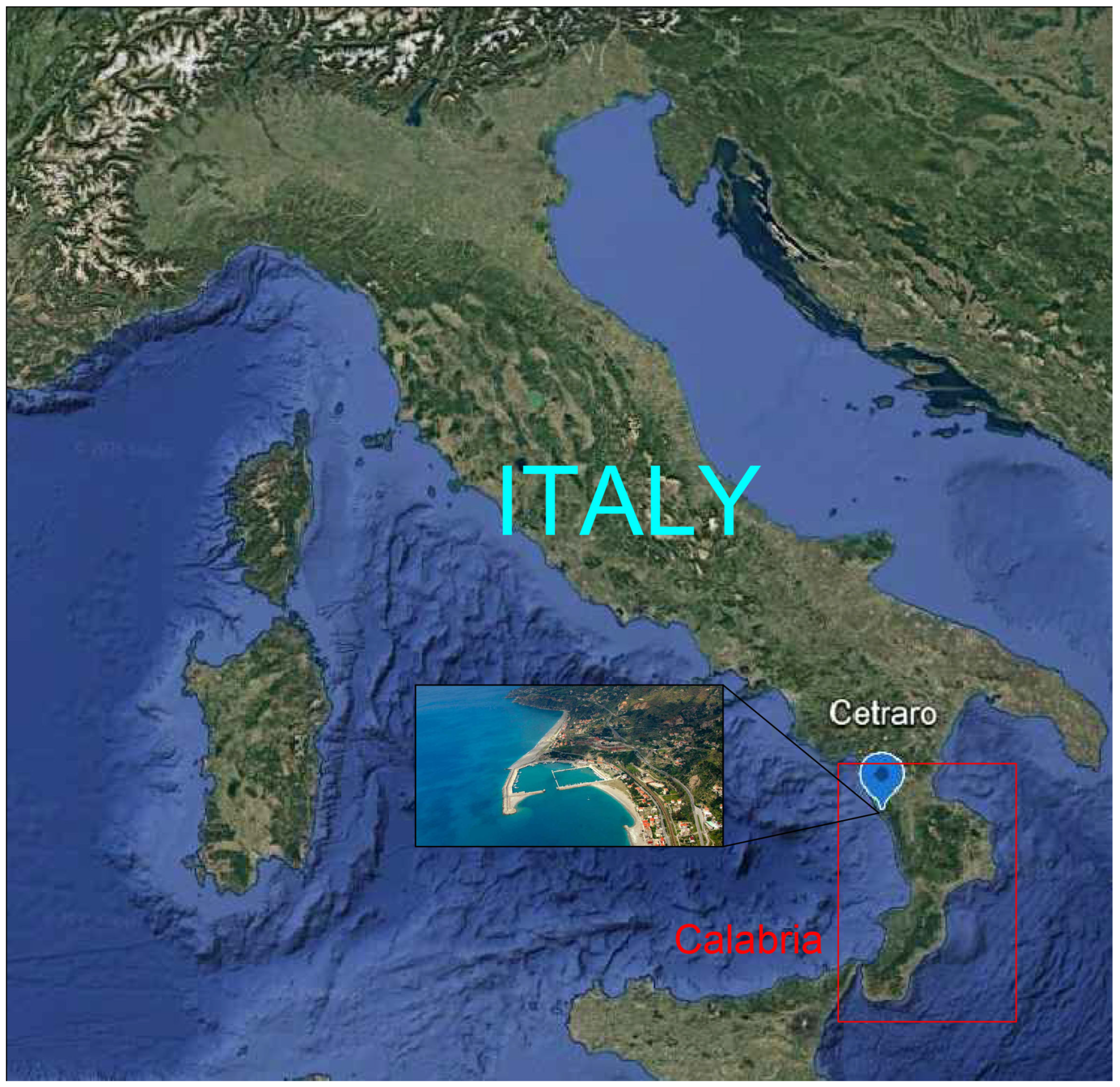
For the purpose of analyzing coastal flooding scenarios in the absence and presence of the REWEC1 system protecting the Cetraro coast, a study of the coastal area was required in order to determine the deep water wave forcing conditions used as input. In this framework, historical wave data series derived from the MeteOcean hindcast database of the Department of Civil, Chemical and Environmental Engineering of the University of Genoa were considered (e.g., [
36]). This dataset covers the entire Mediterranean basin, with a spatial resolution of 0.1273° in latitude and 0.09° in longitude, and a temporal resolution of 1 h. In particular, the used wave hindcast was validated by various Italian, Spanish, and Greek buoy measurements in the Mediterranean Sea, and used for a large number of analyses on wave climate (e.g., [
37,
38]).
In the present study, the reconstruction node no. 005659 was selected, located at a water depth of 473.3 m and characterized by the following coordinates: latitude 39.45° and longitude 15.874°. In particular, for the period from 1 January 1979 to 31 December 2018, the following synthetic wave parameters were extracted: significant wave height
, peak period
, and mean wave direction
. The historical series were subject to a processing procedure aimed at quality control and the removal of inconsistent wave parameters [
29]. The data efficiency, defined as the ratio between filtered and raw data, was equal to 99.68%. Since the reconstruction node is located at a distance of approximately 9 km from the Cetraro coastal area, no geographical transposition was required.
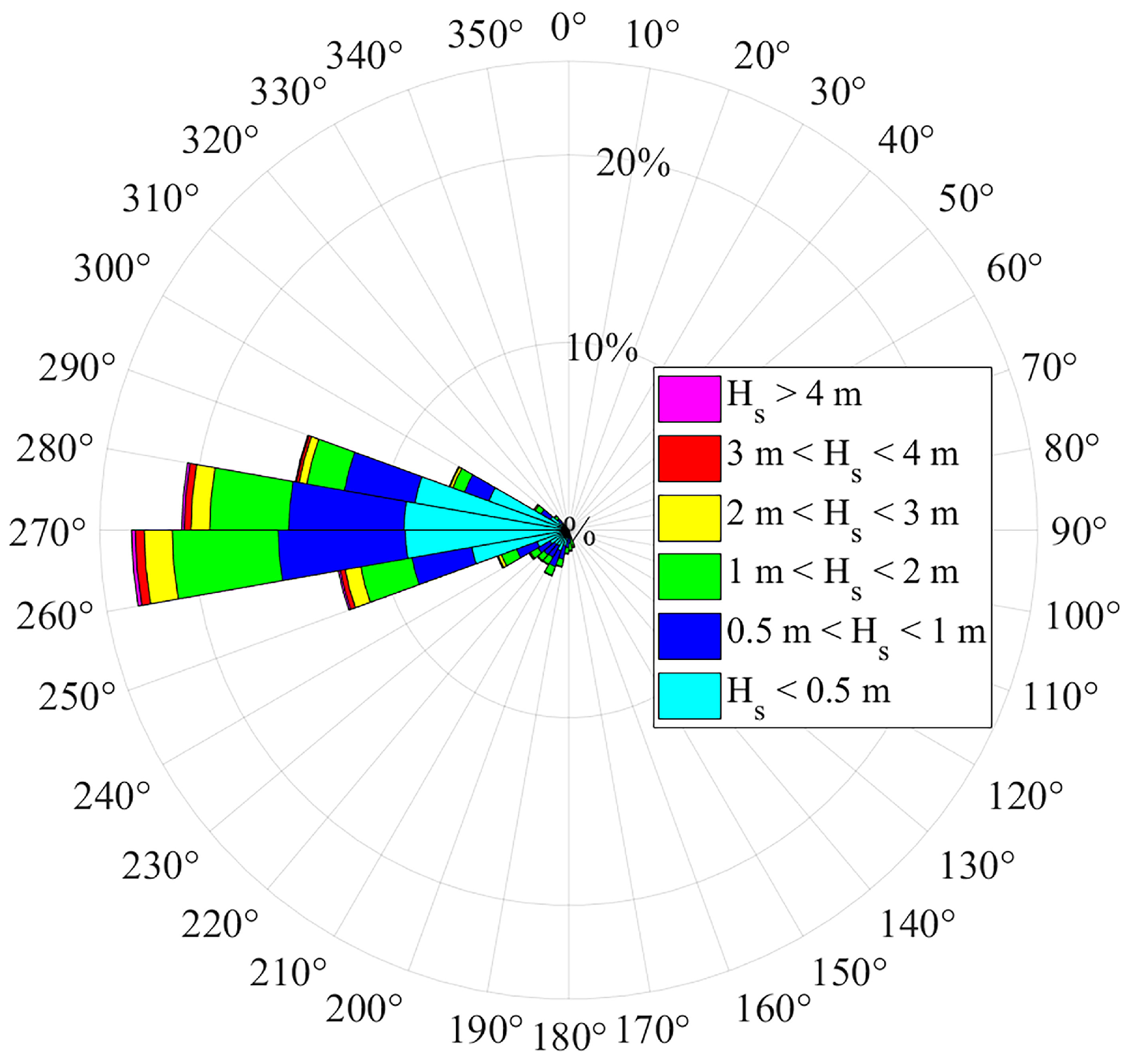
Figure 4 shows the directional wave rose derived from the historical wave data series of the selected reconstruction node, considering only sea states associated with the cross-shore exposure sector of the Cetraro coast (160°–320°). This figure illustrates the percentages of occurrence of wave events, classified into 10° directional sectors and different ranges of
. The most frequent sea states are associated, in decreasing order, with the 260°–270°, 270°–280°, 280°–290°, and 250°–260° directional sectors, with occurrence percentages of 23.31%, 20.63%, 14.80%, and 12.47%, respectively. With reference to the
intervals defined in
Figure 4, the corresponding occurrence percentages are 45% for
< 0.5 m, 28.36% for 0.5 m <
< 1 m, 20.11% for 1 m <
< 2 m, 4.61% for 2 m <
< 3 m, 1.37% for 3 m <
< 4 m, and 0.55% for
> 4 m.
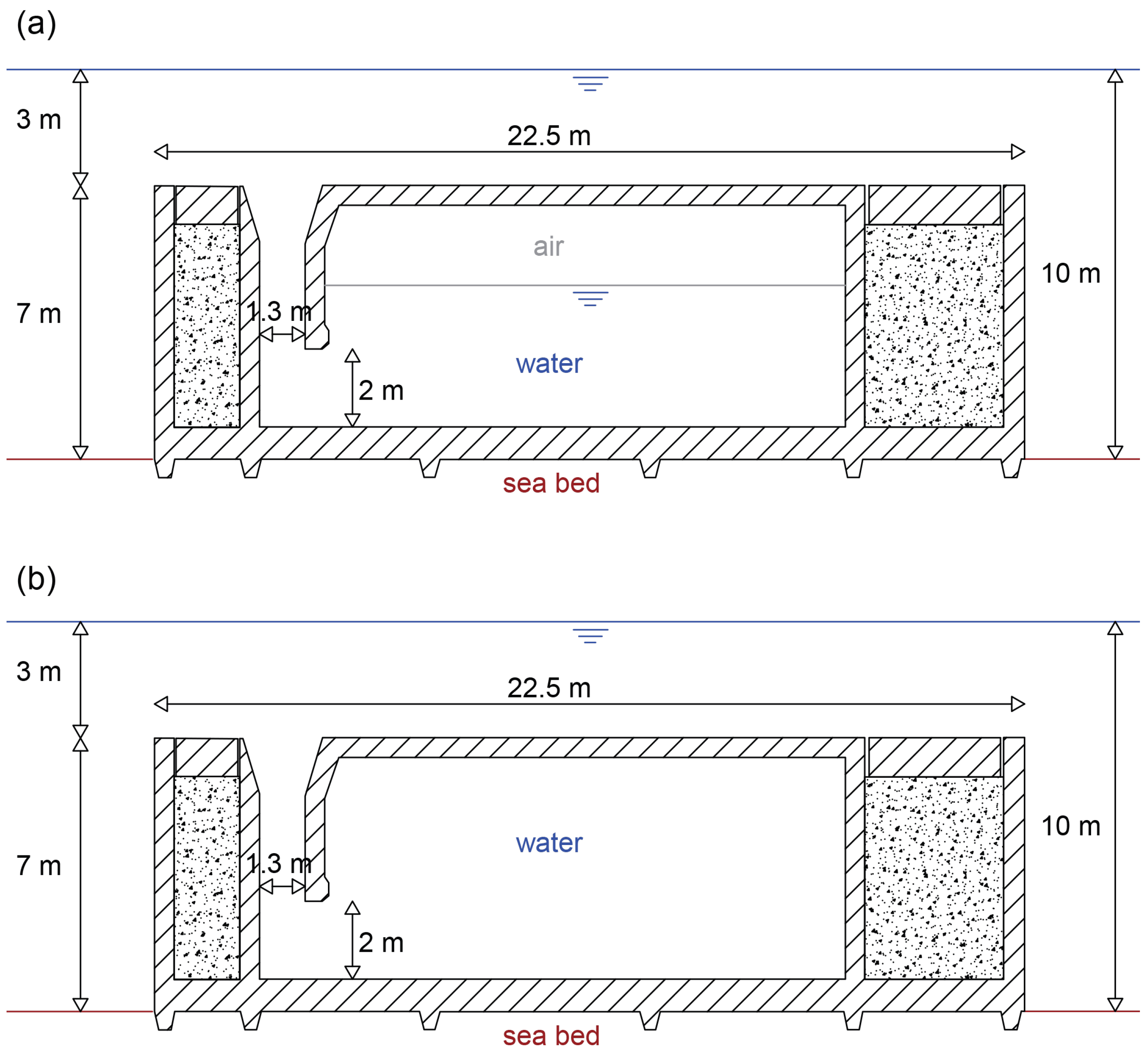
The fixed-air operation of the REWEC1 was investigated using offshore wave conditions corresponding to the 95th percentile (P95) of , since the nearshore propagation of this sea state to the installation depth of 10 m yielded values of close to the resonance condition of the device, associated with maximum energy absorption. The resulting value was 2.17 m.
In contrast, the no-air operation of the REWEC1 was analyzed using design waves with different return periods (
T = 25, 50, and 100 years), representative of extreme sea states. To this end, the following procedure was carried out. First, the historical storm events impacting the Cetraro coastal area were identified using the Peaks-Over-Threshold (POT) method, by imposing a significant wave height threshold equal to 3.5 m. This threshold ensured a sufficient number of storm events for a robust estimation of the design waves. From the
time series, storm events were identified when
exceeded the above-mentioned threshold for a minimum persistence of 6 h and when the wave directions remained confined within an angular sector not exceeding 30° [
39]. Storm intensity was characterized by the maximum significant wave height occurring during each storm event. Based on the highest number of storm events (2161), the 250°–280° directional sector was selected for the determination of the design waves. The determination of design waves was carried out using the method proposed by Goda [
40], which considers both the Gumbel and Weibull probability distributions, with the Weibull shape parameter
k set equal to 0.75, 1, 1.4, and 2. For the selected directional sector (250°–280°), the Weibull distribution with
k = 1 was adopted, as it provided the best correlation between the significant wave height at the storm peak and the reduced variate associated with the non-exceedance probability. The values of
associated with
T = 25, 50, and 100 years are equal to 8.74 m, 9.23 m, and 9.72 m, respectively, for the 250°–280° directional sector.
The peak wave period associated with P95 of
was determined using a conditional statistical approach (e.g., [
41]). Then, a representative
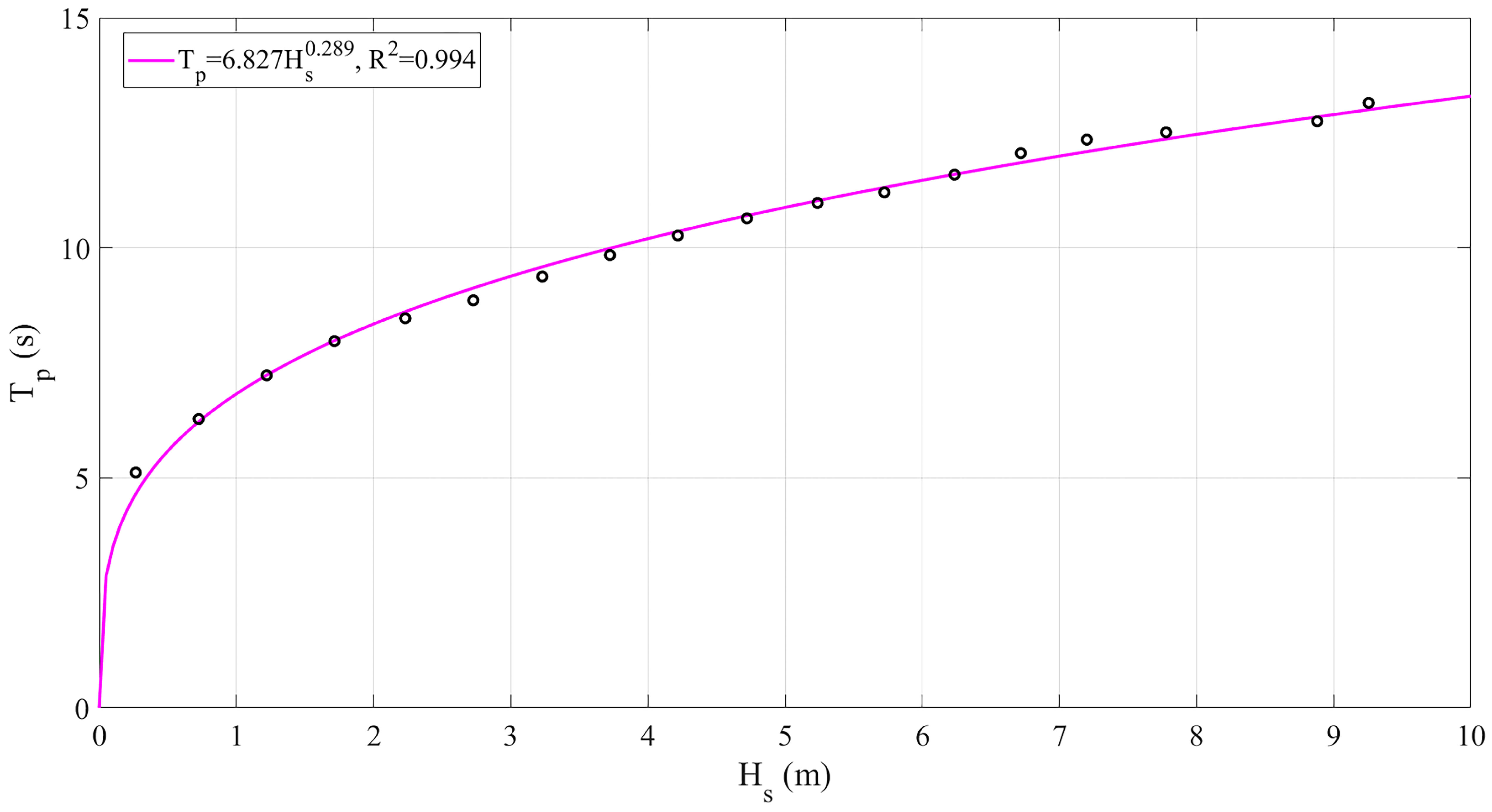
of 8.7 s was derived from the resulting conditional distribution. The peak period values associated with the selected design waves within the chosen directional sector were derived by means of a power-law relationship of the form
=
. This relationship was obtained by interpolating the mean values of
computed over 0.5 m intervals and the corresponding mean values of
associated with the same intervals. As shown in
Figure 5, the resulting curve was a good fit with the mean wave data with a correlation coefficient
equal to 0.994. The calibrated parameters
and
were found to be equal to 6.827 and 0.289, respectively. Based on the calibrated power-law curve, the values of
associated with
for
T = 25, 50, and 100 years were obtained, namely 12.77 s, 12.98 s, and 13.17 s.
The representative wave direction associated with the P95 of
was determined by computing the circular mean of wave directions corresponding to all sea states with
≥ P95 [
42]. Under this approach, the resulting
was equal to 267.2°. The directions of the selected design waves were determined using the one-to-one quantile method [
43], which allows the design wave to be associated with the real storm event whose significant wave height most closely matches the estimated extreme value. Therefore, the design wave directions were assumed to be equal to those of the observed event closest to the design condition. For the selected 250°–280° directional sector, the resulting
values for
T = 25, 50, and 100 years were 271.2°, 264.3°, and 263.7°, respectively.
5.2. Nearshore Wave Propagation
The offshore P95 of
and the design waves with return periods
T = 25, 50, and 100 years were propagated toward the nearshore zone in correspondence with the Cetraro coast using the SWAN model. The application of this model required the representation of the seabed morphology in front of the investigated coast. For the construction of an appropriate computational grid containing bathymetric information, bathymetric data were derived from nautical charts provided by the Italian Hydrographic Institute for deeper waters and from dedicated nearshore topo-bathymetric surveys with a spatial resolution of 0.5 m, carried out by the Department of Biology, Ecology and Earth Sciences of the University of Calabria (e.g., [
27]). The spatial domain adopted for the SWAN computational grid was characterized by a length
x = 10,800 m and a width
y = 4200 m. The transformation of the bathymetric data into computational cells, with dimensions
=
= 15 m and assigned depth values, was performed using the software Surfer through a Kriging-type spatial interpolation [
44].
Based on the offshore wave conditions and on the specific bathymetry of the study area, the SWAN model was initially applied in a baseline configuration without REWEC1 to derive, at the water depth of 10 m where these devices were placed, the characteristics of the incident wave field under undisturbed conditions. The input design waves were modeled using a two-dimensional JONSWAP spectrum with a spectral peak enhancement factor
= 3.3 and a directional spreading parameter
s = 10. From the SWAN propagation results obtained at the 10 m depth in the absence of REWEC1, the values of
were derived to determine the transmission
and reflection
coefficients of the REWEC1 devices operating in fixed-air and no-air modes, as a function of the specific wave forcing. These parameters allow the hydraulic characterization of the devices in subsequent SWAN simulations, accounting for their presence. Although SLR modifies the relative submergence of submerged structures and may affect their hydraulic performance, in the present study, the transmission and reflection coefficients were kept unchanged. SLR was accounted for exclusively as an increase in the mean water level and superimposed on the wave conditions in the successive flooding simulations. This approach is consistent with common practice in coastal flooding assessments, where future SLR is incorporated as a shift in the hydrodynamic boundary conditions rather than through a reparameterization of wave–structure interaction processes (e.g., [
45,
46]). Therefore, the resulting analysis provides a conservative estimate of the mitigation performance of the REWEC1 devices.
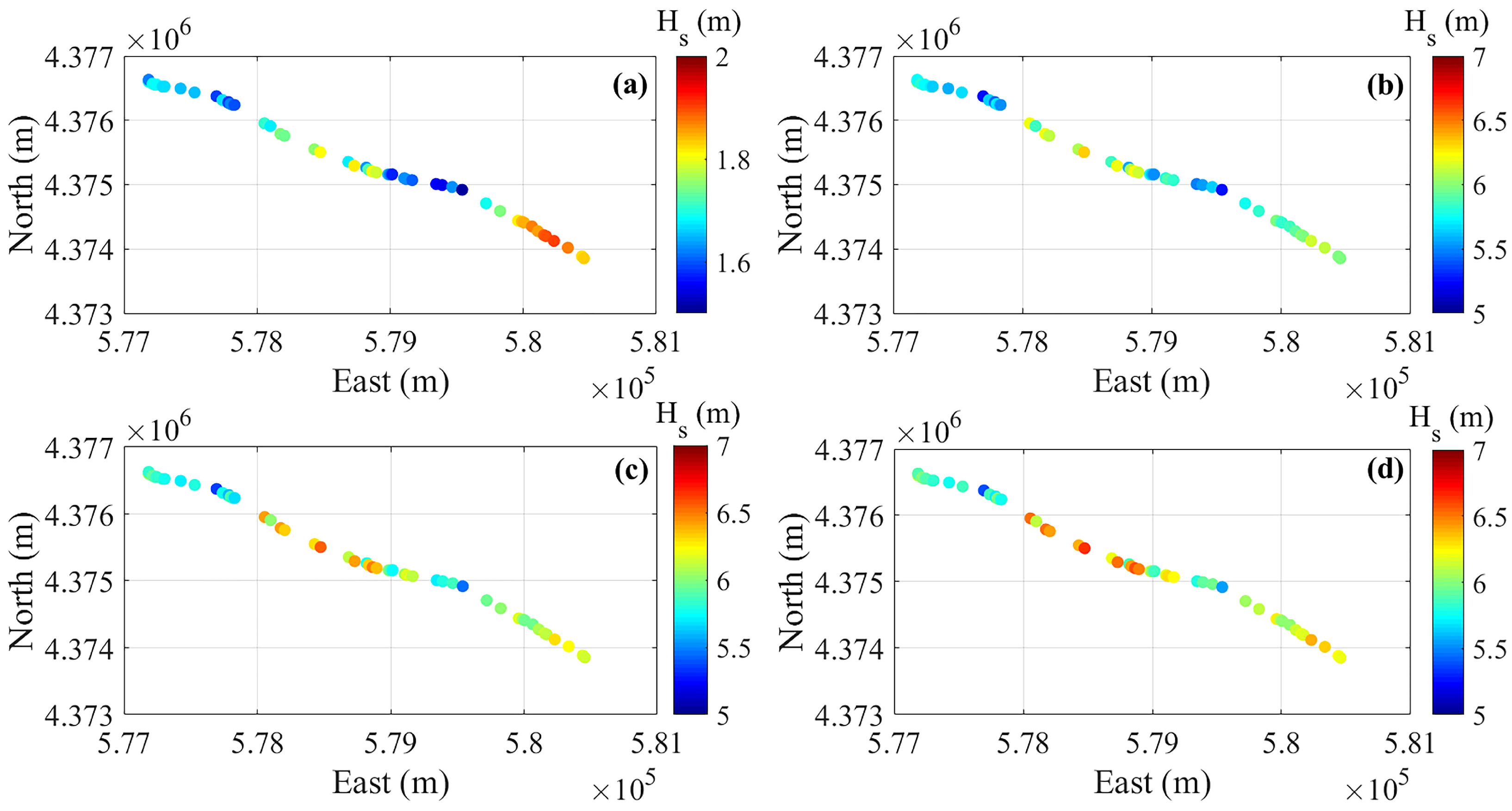
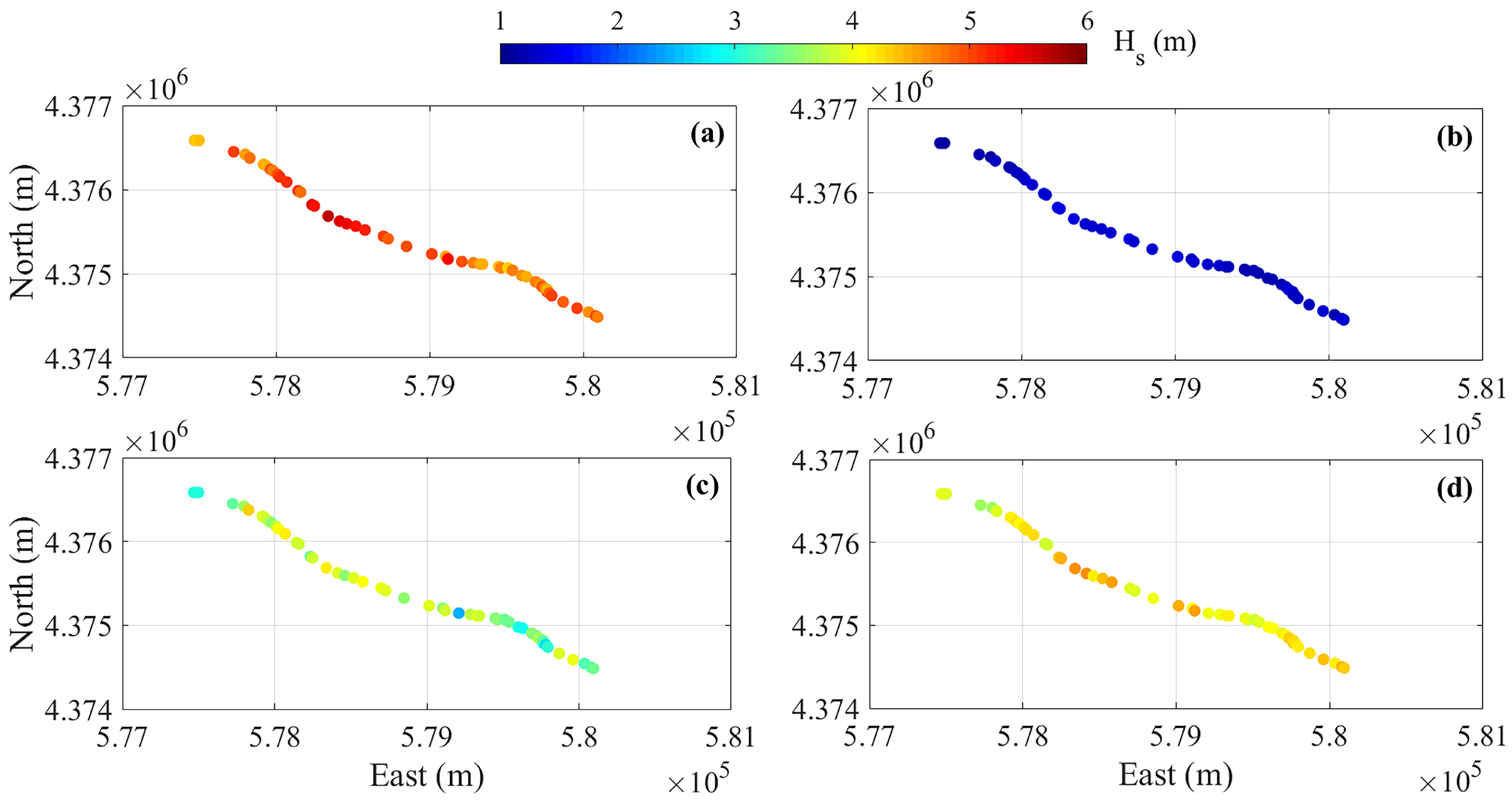
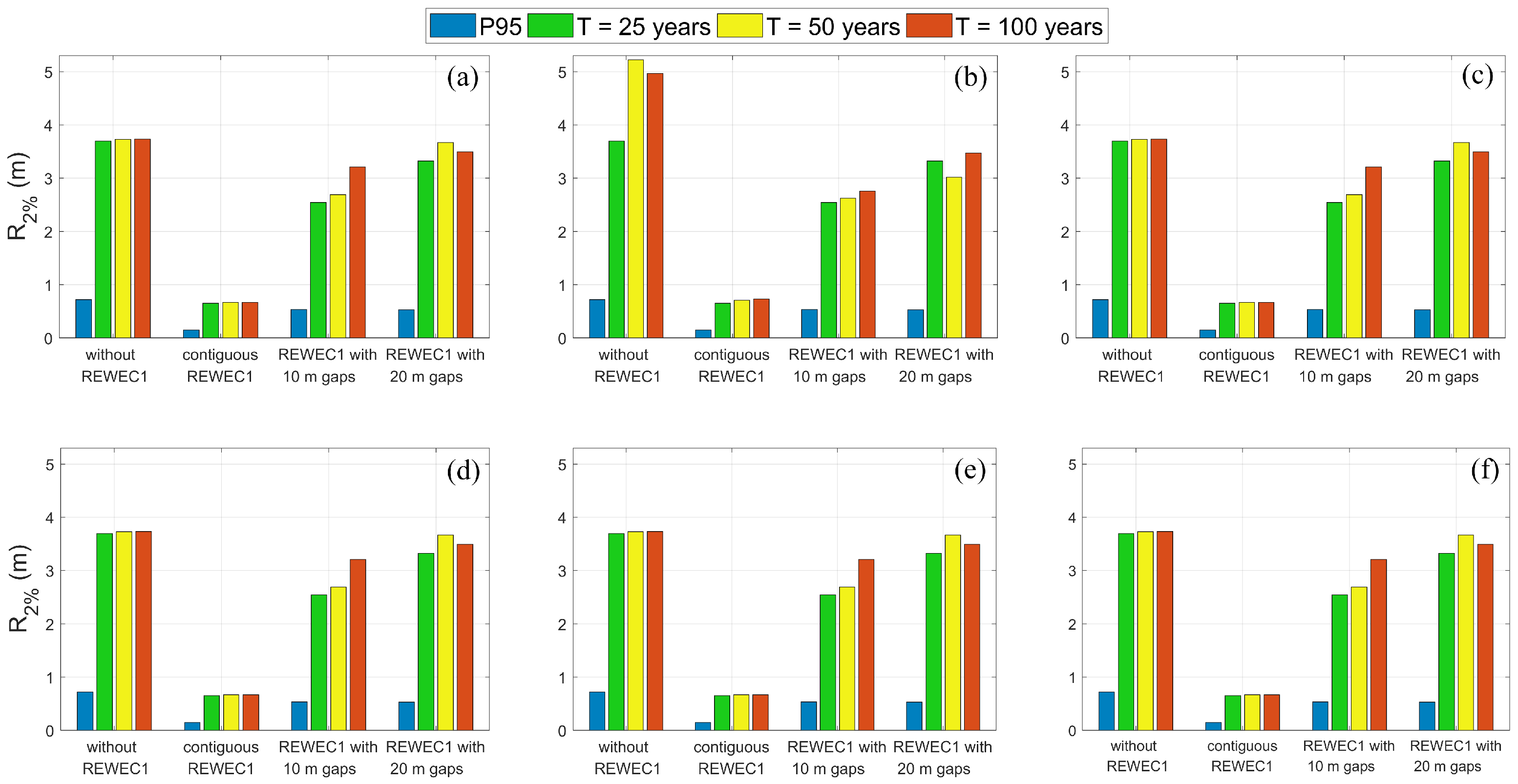
Figure 6 shows the variation of
along the computational nodes closest to the 10 m depth contour, identified with a vertical tolerance of 0.05 m. The results refer to the P95 of
(
Figure 6a), characterized offshore by
= 2.17 m,
= 8.7 s, and
= 267.2°; to the design wave with
T = 25 years (
Figure 6b), characterized offshore by
= 8.74 m,
= 12.77 s, and
= 271.2°; to the design wave with
T = 50 years (
Figure 6c), characterized offshore by
= 9.24 m,
= 12.98 s, and
= 264.3°; and to the design wave with
T = 100 years (
Figure 6d), characterized offshore by
= 9.72 m,
= 13.17 s, and
= 263.7°. For the selected water depth, the values of
range from 1.51 m to 1.90 m for the P95 of
, from 5.29 m to 6.43 m for the design wave with
T = 25 years, from 5.35 m to 6.53 m for the design wave with
T = 50 years, and from 5.40 m to 6.64 m for the design wave with
T = 100 years.
As shown in
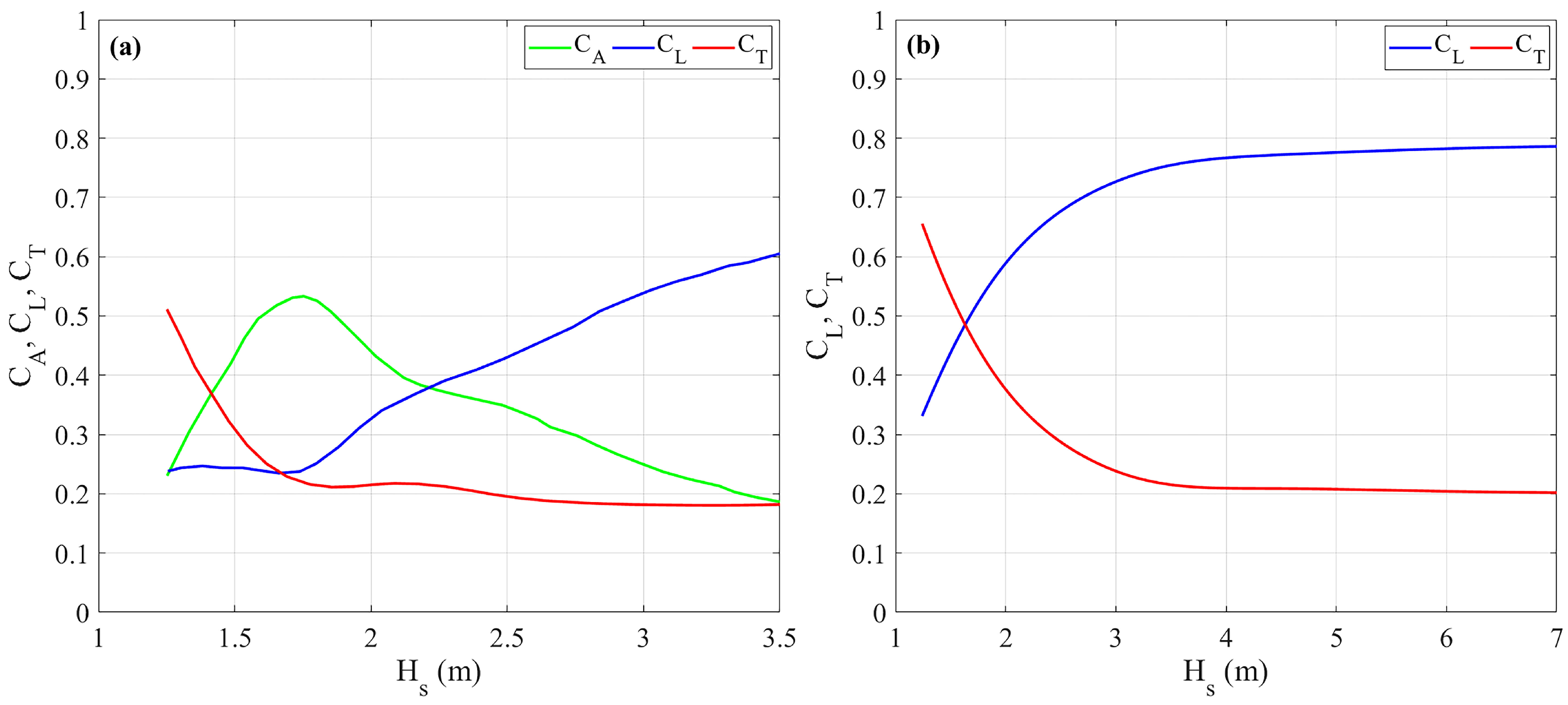
Figure 2, the values of
and
were derived as a function of the variability of
at a water depth of 10 m for each wave attack and REWEC1 operating mode, while the corresponding values of
were obtained from the energy balance, as described in
Section 2. For the P95 of
,
oscillates between 0.43 and 0.53,
oscillates between 0.21 and 0.31,
between 0.24 and 0.31, and
between 0.009 and 0.021. For the design wave with
T = 25 years,
oscillates between 0.203 and 0.207,
between 0.778 and 0.784, and
between 0.009 and 0.019. For the design wave with
T = 50 years,
oscillates between 0.202 and 0.206,
between 0.780 and 0.785, and
between 0.009 and 0.018. For the design wave with
T = 100 years,
oscillates between 0.201 and 0.205,
between 0.781 and 0.787, and
between 0.008 and 0.018. Owing to the relatively high values of
associated with the selected design waves, only limited variations of these coefficients are observed.
The values of
and
enabled the characterization of the hydraulic performance of the REWEC1 devices, which can be represented in SWAN as rigid obstacles whose heads may be positioned within the computational domain at locations not necessarily coincident with the grid nodes [
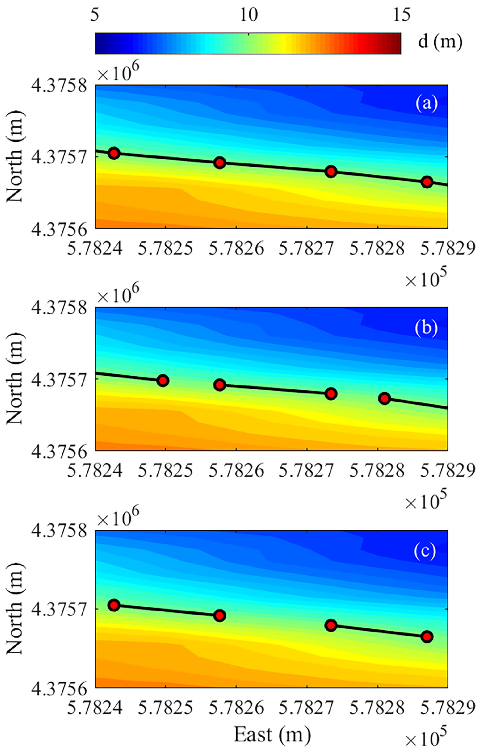
47]. In this framework, for each wave attack and at a water depth of 10 m (vertical tolerance of 0.05 m), three different spatial configurations of the REWEC1 devices were tested
Configuration 1: array of contiguous REWEC1 units, each 20 m long;
Configuration 2: array of 20 m long REWEC1 units with 10 m wide gaps;
Configuration 3: array of 20 m long REWEC1 units with 20 m wide gaps.
The choice of the gap length between devices for configurations 2 and 3 follows typical design criteria for detached rubble-mound breakwaters for coastal protection, according to which the gap length should range between 0.5 and 2 times the length of the barrier (e.g., [
48,
49]).
The obstacle arrangement procedure adopted to simulate the REWEC1 units within the SWAN computational domain consisted of four main steps. First, the target isobath at a water depth of 10 m was extracted from the bathymetric grid by identifying grid cells intersected by the selected depth contour and computing the corresponding contour segments through linear interpolation. Second, the contour segments were merged by removing duplicate nodes and assembling them into a graph structure, which was used to reconstruct continuous polylines representing the isobath geometry. Third, each polyline was parameterized along its curvilinear coordinate by computing the cumulative distance. Finally, obstacles were generated by sampling the curvilinear abscissa and defining straight segments with a fixed length of 20 m, separated by either zero gap (continuous configuration) or constant gaps of 10 m and 20 m. This procedure was specifically designed to generate obstacle geometries suitable for implementation in the SWAN model, ensuring a consistent representation of obstacle length, spacing, and alignment with the local isobath geometry. In the SWAN model, the values of
and
obtained at a water depth of 10 m as a function of
were assigned to the individual obstacles representing the REWEC1 devices, based on their positioning within the three tested spatial configurations. A representative detail of the three adopted REWEC1 configurations, including the bathymetry around the 10 m water depth, is shown in
Figure 7.
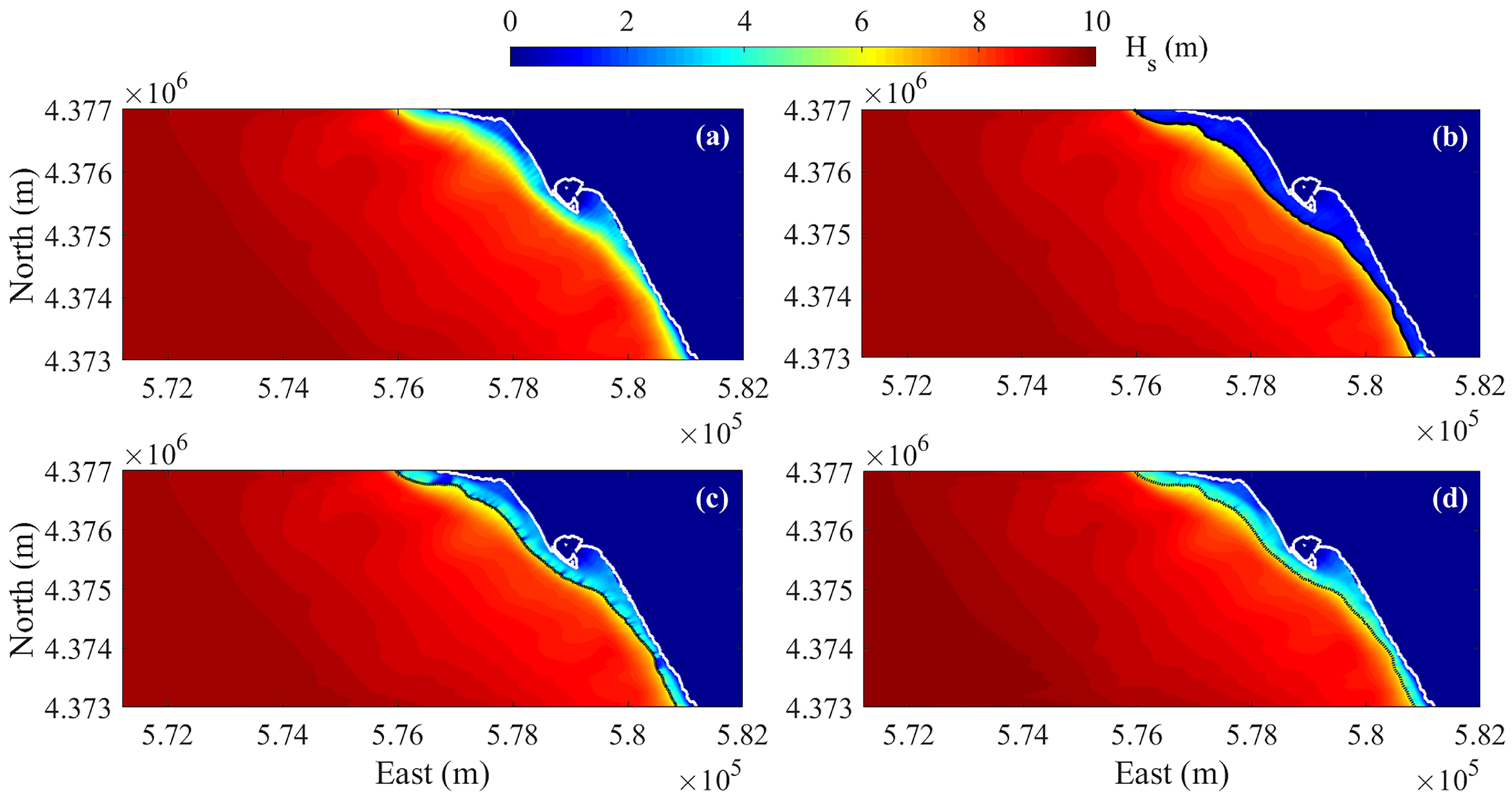
The results of the SWAN numerical simulations are shown in
Figure 8 in terms of the spatial variation of
for the representative and most variable case, corresponding to the design wave with
T = 100 years. The figure compares undisturbed conditions (without REWEC1), configuration 1 (contiguous REWEC1), configuration 2 (REWEC1 with 10 m gaps), and configuration 3 (REWEC1 with 20 m gaps). The shoreline is indicated by a white line, whereas, in the subplots referring to the three REWEC1 spatial configurations, the units are highlighted by black lines. As observed, the attenuation of
in the lee of the REWEC1 devices varies depending on their spatial configuration, in comparison with the baseline configuration characterized by undisturbed conditions (
Figure 8a). In configuration 1 (
Figure 8b), where the REWEC1 units are arranged contiguously, a substantial reduction of
(approximately 80% immediately downstream of the devices) is observed, as a consequence of transmission coefficients on the order of 0.2. Due to the contiguous arrangement of the devices, this attenuation is spatially distributed in a nearly uniform manner in their lee. In configuration 2 (
Figure 8c), where the REWEC1 units are arranged with 10 m wide gaps, the
values in the sheltered area exhibit a marked spatial heterogeneity. The presence of 10 m gaps between adjacent REWEC1 modules allows part of the wave energy to propagate downstream through diffraction processes. This modular arrangement with gaps implies a combined effect of energy dissipation due to wave breaking at the modules and wave propagation through the gaps. Overall, the significant wave height is, on average, reduced within the area protected by the REWEC1 array. In configuration 3 (
Figure 8d), characterized by 20 m wide gaps between the REWEC1 units, a greater spatial homogeneity of
values downstream of the devices is observed compared to the case with 10 m gaps. The increased homogeneity of the wave field in the lee of the REWEC1 array with wider gaps is a direct consequence of the dominance of diffraction and wave propagation processes. As the gap width increases, the portion of the wave front passing through the gaps spreads more effectively, dispersing energy over a wider area and with a larger angular extent. In this context, the interference between waves diffracted from the two ends of a gap and from successive gaps tends to overlap more uniformly, smoothing the differences between the area immediately behind the REWEC1 units and the area immediately behind the gaps, where maximum wave transmission occurs.
However, the SWAN numerical model does not allow for the simulation of coastal flooding processes. For this reason, a second numerical model was required to investigate these processes and assess the impact of REWEC1 farms on mitigating coastal flooding risk. In the present study, the SWAN results, obtained both in the absence and in the presence of REWEC1 under the different spatial configurations, were provided as input to the subsequent XBeach hydro-morphodynamic model capable of simulating coastal inundation processes. Considering the placement of the REWEC1 devices at a water depth of 10 m, the values of
,
, and
simulated by SWAN under fixed-air and no-air operating modes, and for different configurations (absence of REWEC1, contiguous REWEC1, REWEC1 with 10 m gaps, and REWEC1 with 20 m gaps) were extracted in the lee of the devices, i.e., at a depth of 7 m, to account for the specific wave field resulting from the interaction with the devices. Considering the design wave with
T = 100 years as a representative case,
Figure 9 shows the trends of
at a set of computational nodes closest to the 7 m depth contour, identified within a vertical tolerance of 0.05 m. A strong variation of
among the different configurations can be observed, with values progressively decreasing from the configuration without REWEC1 (
Figure 9a) to the configuration with contiguous REWEC1 units (
Figure 9b). Configurations characterized by REWEC1 units with 10 m gaps (
Figure 9c) and 20 m gaps (
Figure 9d) exhibit a higher spatial variability of
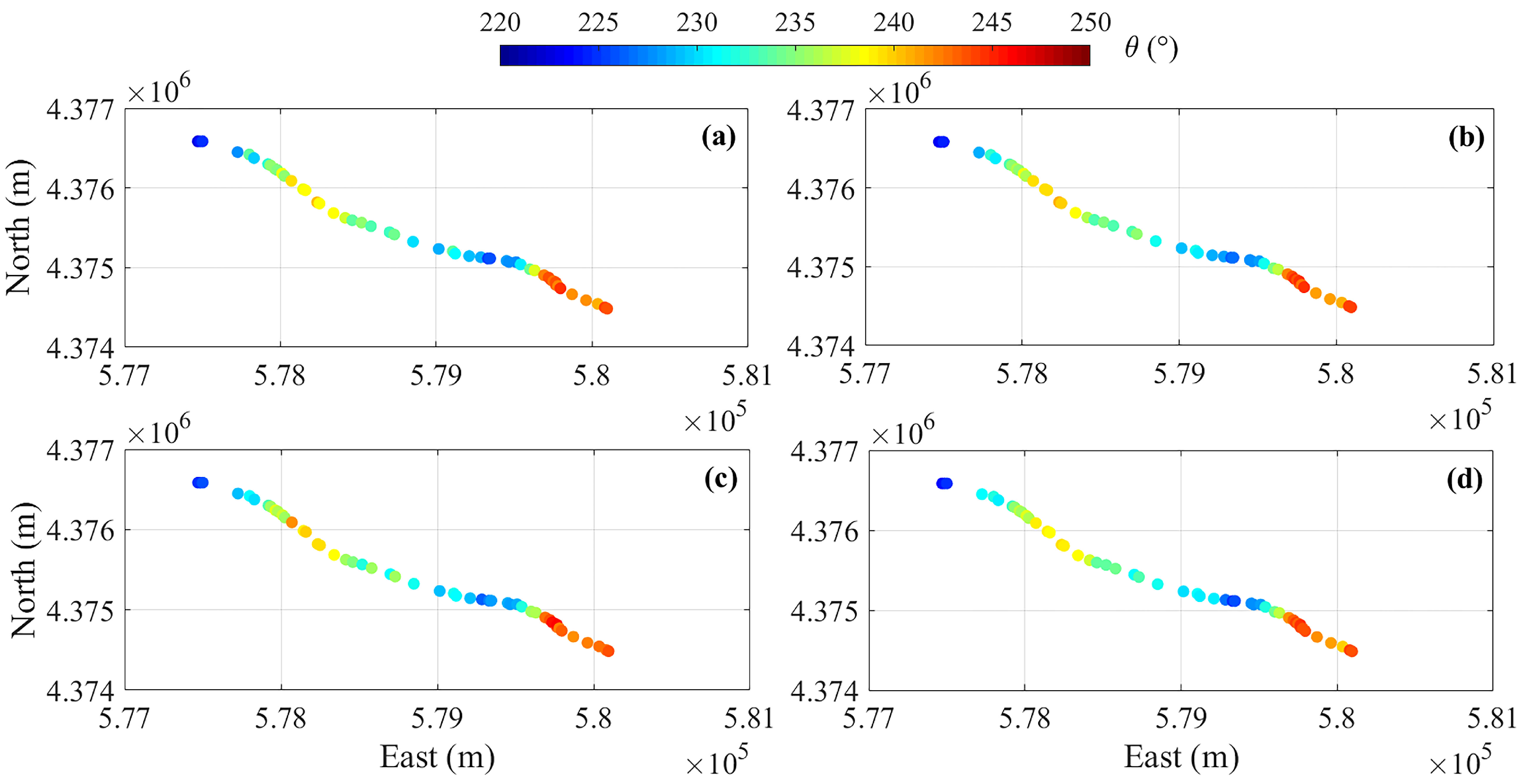
values along the computational domain compared to the other configurations. Concerning the mean wave direction
(
Figure 10), the spatial variability among the different configurations is fairly similar, although slightly larger oscillations are observed in the presence of REWEC1 devices with gaps (
Figure 10c,d). As for the peak period
, it remains unchanged at the 7 m depth with respect to offshore conditions in the absence of REWEC1, whereas in the presence of REWEC1 it exhibits a slight increase (ranging between 1% and 2%). This behavior is because the devices tend to attenuate high-frequency spectral components to a relatively greater extent than low-frequency components, producing a slight shift of the spectral peak toward longer periods.
5.3. Coastal Flooding
The results in terms of significant wave height
, peak period
, and mean wave direction
at a water depth of 7 m, obtained for the fixed-air and no-air operating modes of REWEC1, were used as input to the hydro-morphodynamic numerical model XBeach [
26]. To limit the number of numerical simulations while preserving a conservative assessment of future conditions, a single high-end SLR scenario was considered. The RCP8.5 projection for the year 2100 was adopted and superimposed on the wave-induced flooding scenarios, including frequent wave conditions (P95 of
) under fixed-air operation and extreme storm events with 25-, 50-, and 100-year return periods under no-air operation. SLR projection under the RCP8.5 scenario was obtained from the NASA Sea Level Projection Tool (sealevel.nasa.gov/ipcc-ar6-sea-level-projection-tool), which provides access to global and regional sea level projections from the IPCC Sixth Assessment Report [
50]. Based on the IPCC RCP8.5 projections, a SLR of 0.78 m was found for the study area.
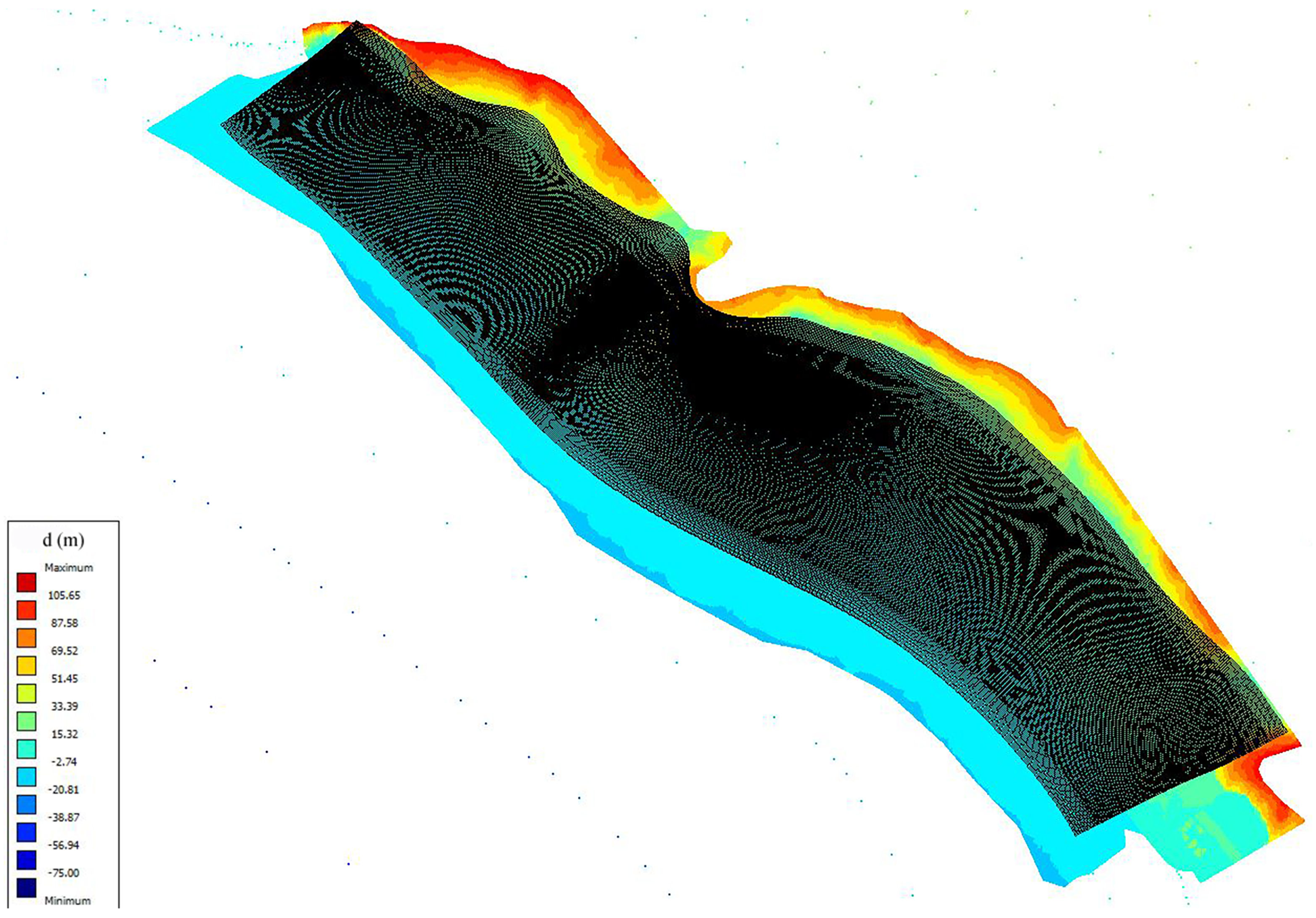
The first step in the application of the XBeach model consisted of defining the computational grid using the Delft3D software package [
51]. As for the SWAN model, grid construction was based on topographic and bathymetric data derived from nautical charts provided by the Italian Hydrographic Institute and from dedicated nearshore topo-bathymetric surveys conducted by the Department of Biology, Ecology and Earth Sciences of the University of Calabria (e.g., [
27]). In addition, the topography of a portion of the emerged coast was reconstructed using LIDAR data available from the National Geoportal of the Italian Ministry for the Environment and Energy Security (gn.mase.gov.it/portale/home), with a spatial resolution of 1 m.
Based on these datasets, a curvilinear computational grid was generated, extending from the −7 m depth contour offshore to elevations inland exceeding the maximum expected flooding levels. The grid consists of
computational nodes, with spatial resolution varying between 10 m and 1 m. Grid refinement was applied in the vicinity of the shoreline in order to achieve a higher level of detail in the simulation of nearshore hydrodynamic processes.
Figure 11 shows the topography of the emerged and submerged coastal areas, together with the curvilinear grid adopted for the Cetraro coast to run XBeach simulations.
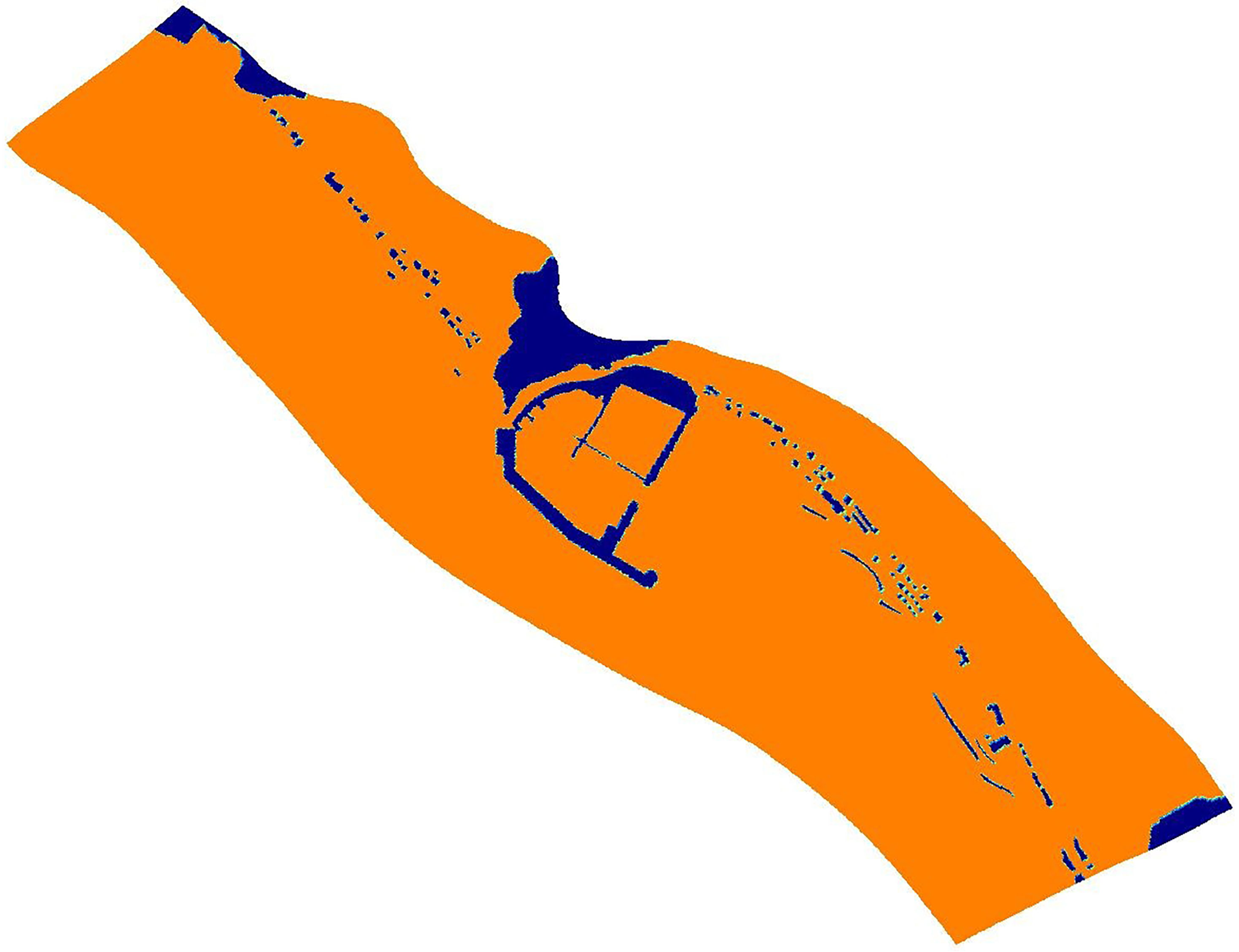
To optimize the numerical simulations performed with XBeach, particular care was devoted to the definition of non-erodible computational cells, representing the port infrastructure of Cetraro, the breakwaters located South of the port, various coastal civil infrastructures, and rocky outcrops of the emerged coast. A detailed representation of these elements is provided in
Figure 12.
The offshore boundary conditions for XBeach were specified at each grid node along the offshore boundary of the computational domain by interpolating the wave parameters (, , and ) obtained from the SWAN simulations at a water depth of 7 m. As for the SWAN model, the input two-dimensional JONSWAP spectrum was defined using and . To characterize the sediment properties of the study area, a median grain size mm and a 90th percentile grain size mm were adopted. These values were derived from a recent granulometric survey campaign carried out by the Municipality of Cetraro within a project aimed at assessing the morphodynamic functionality of the port.
The duration of the XBeach simulations, aimed at analyzing maximum coastal flooding both in the absence and presence of REWEC1 devices, was set equal to 6 h in order to balance physical realism and computational cost. Preliminary analyses showed that longer simulation times did not lead to significant changes in the main engineering-relevant variables related to coastal flooding, such as maximum inundated areas, maximum inland water penetration, and wave set-up and run-up values.
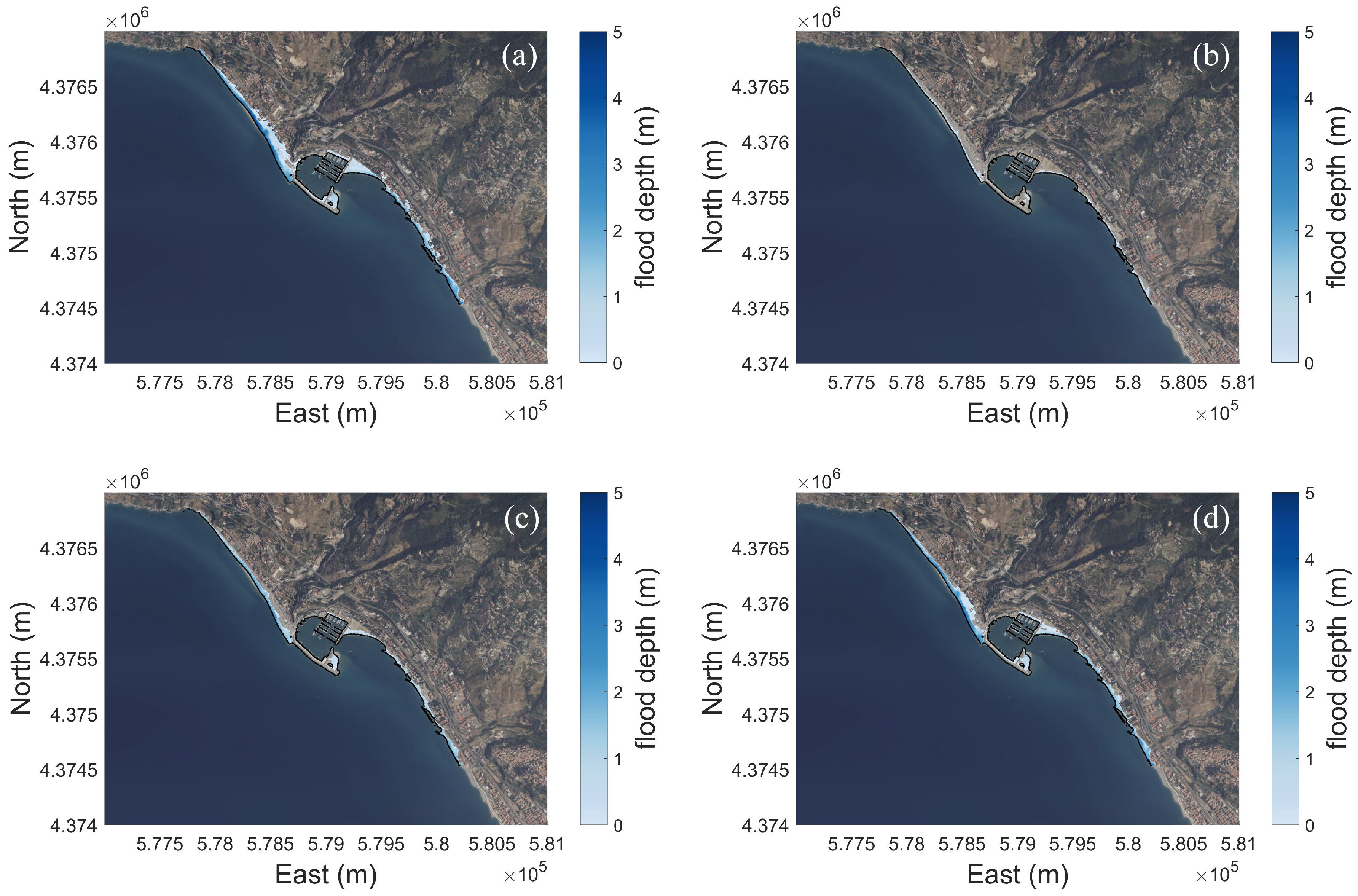
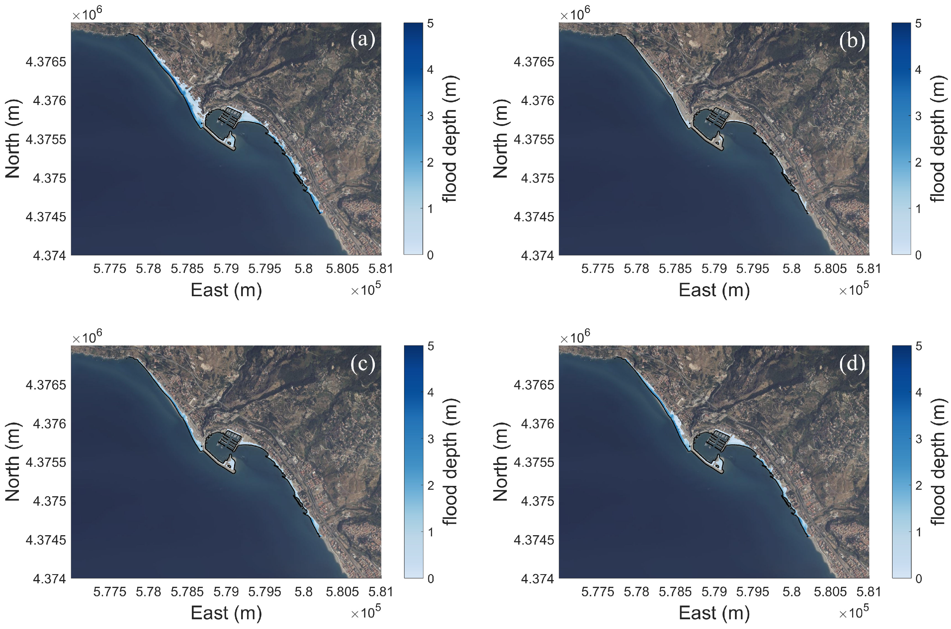
Figure 13,
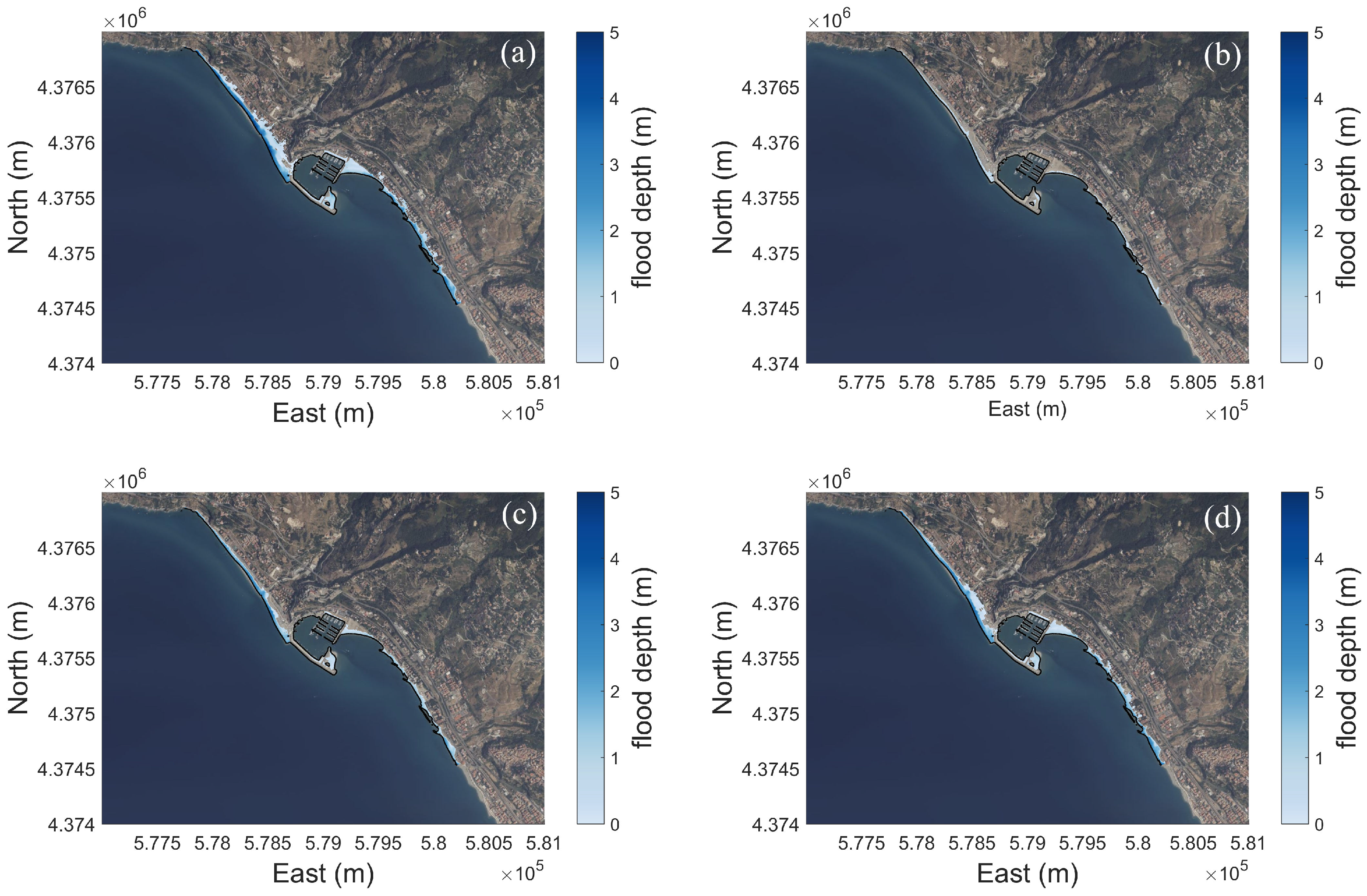
Figure 14 and
Figure 15 show the XBeach simulation results in terms of the spatial distribution of maximum flood depths over the emerged coastal area for the design waves with
T = 25, 50, and 100 years, respectively, combined with RCP8.5 SLR, and for the different spatial configurations considered (absence of REWEC1, contiguous REWEC1 arrays, REWEC1 with 10 m gaps, and REWEC1 with 20 m gaps). Owing to their limited spatial extent, the inundation maps associated with the P95 of
, combined with RCP8.5 SLR, were not shown; their effects were instead analyzed in terms of maximum inundated areas, maximum inland water penetration, and wave set-up and run-up in the subsequent analyses. The flooding scenarios, highlighted in
Figure 13,
Figure 14 and
Figure 15, represent the most unfavorable conditions, i.e., the maximum flood depths reached at each computational cell during the simulation time. Accordingly, inundated areas and inland water penetration distances refer to their maximum spatial extent. It should be noted that the background orthophoto used for visualization does not correspond temporally to the shoreline position considered in this study, which is indicated by a black line and derived from the topo-bathymetric surveys carried out by the Department of Biology, Ecology and Earth Sciences of the University of Calabria (e.g., [
27]). Overall, the simulation results exhibit a spatial variability that is strongly dependent on the emerged coastal topography and on the presence of coastal structures and civil infrastructures. North of the port, the coast is characterized by a wide and gently sloping beach that gradually narrows landward. This sector experiences the largest flooding extent along the study area, with inland water penetration strongly influenced by the spatial arrangement of civil infrastructures. South of the port, inundated areas are generally smaller due to the presence of some rubble-mound breakwaters, a narrower beach, and a complex backshore topography. With reference to the meteo-marine forcing conditions shown (design waves combined with RCP8.5 SLR), slightly more severe flooding conditions are associated with the design wave with
T = 100 years in almost all configurations. Compared to the configuration without REWEC1, which exhibits the largest inundated areas, water penetration distances, and flood depths (
Figure 13a,
Figure 14a and
Figure 15a), the presence of REWEC1 devices results in a clear reduction in these quantities due to wave energy dissipation in their lee. In particular, contiguous REWEC1 arrays produce the most significant reduction in inundated areas (
Figure 13b,
Figure 14b and
Figure 15b), followed by configurations with 10 m gaps (
Figure 13c,
Figure 14c and
Figure 15c) and 20 m gaps (
Figure 13d,
Figure 14d and
Figure 15d).
For all spatial configurations,
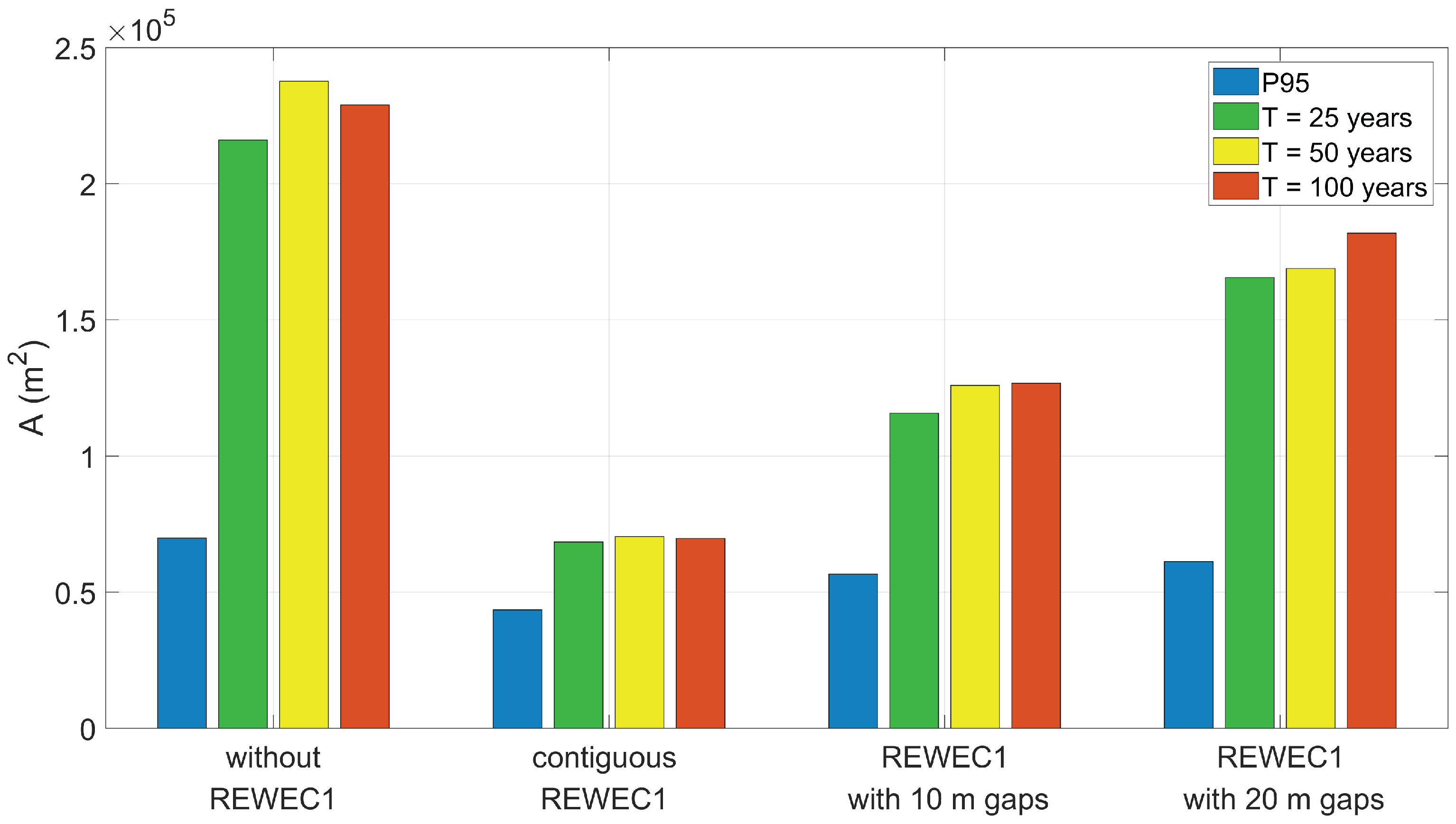
Figure 16 shows the maximum flooded areas
A along the entire coast, distinguishing between cases using the P95 of
and those using design waves with
T = 25, 50, and 100 years, all combined with RCP8.5 SLR. Except for the cases without REWEC1 and with contiguous REWEC1, the highest values of
A are associated with the design wave with
T = 100 years. Progressive reductions in
A occur with the inclusion of REWEC1 devices, from the configuration with 20 m gaps to the contiguous configuration. Moreover, the reduction in
A associated with the selected design wave conditions is essentially similar across all REWEC1 configurations and larger than that associated with P95 of
. This different behavior is related to the more dissipative nature of the REWEC1 in no-air conditions compared to the device operating in fixed-air conditions. It is worth noting that the relatively large extent of flooded areas is associated with the extreme value of the adopted SLR.
A quantitative assessment of the percentage reduction in maximum inundated area due to the presence of REWEC1 devices operating in no-air and fixed-air modes under all meteo-marine forcing conditions is reported in
Table 1. The table defines the relative variation
, where
is the difference between the maximum inundated area in the absence and presence of REWEC1, and
is the maximum inundated area without REWEC1. The results indicate that the percentage reductions in maximum inundated area are more pronounced under design wave conditions than when the P95 of
is used as wave forcing, highlighting the effectiveness of REWEC1 in mitigating coastal flooding during extreme wave events. For all the design wave conditions considered, an average reduction of approximately 69% is observed for contiguous REWEC1 arrays, about 46% for the configuration with 10 m gaps, and about 24% for the configuration with 20 m gaps.
Similarly,
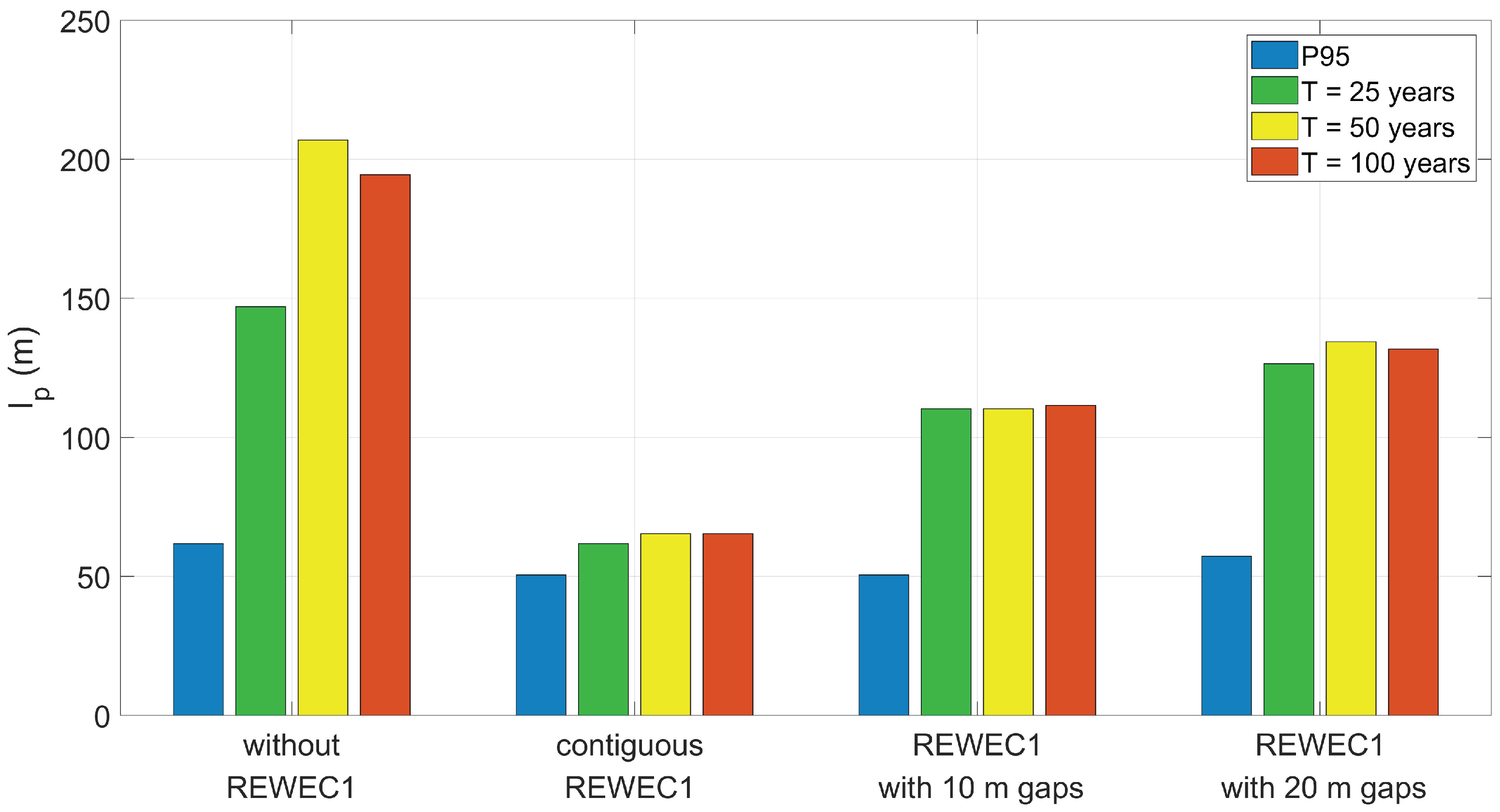
Figure 17 presents the maximum inland water penetration lengths
for the different configurations and the adopted wave conditions (P95 of
and design waves with
T = 25, 50, and 100 years), all combined with RCP8.5 SLR. The values range from maximum values of approximately 200 m in the absence of REWEC1 to values slightly above 50 m for the contiguous configuration, exhibiting trends comparable to those observed for the maximum inundated areas under the different wave conditions. Also in this case, SLR appears to play a relevant role in the assessment of
.
Table 2 reports the relative reduction
, where
is the difference between the maximum penetration length in the absence and presence of REWEC1, and
is the maximum penetration length without REWEC1. The results highlight a progressive attenuation of inland water penetration from the configuration with 20 m gaps to that with contiguous devices. The reduction percentages are quite comparable to those obtained for inundated areas (with mean variations of a few percentage points), being more pronounced under design wave conditions.
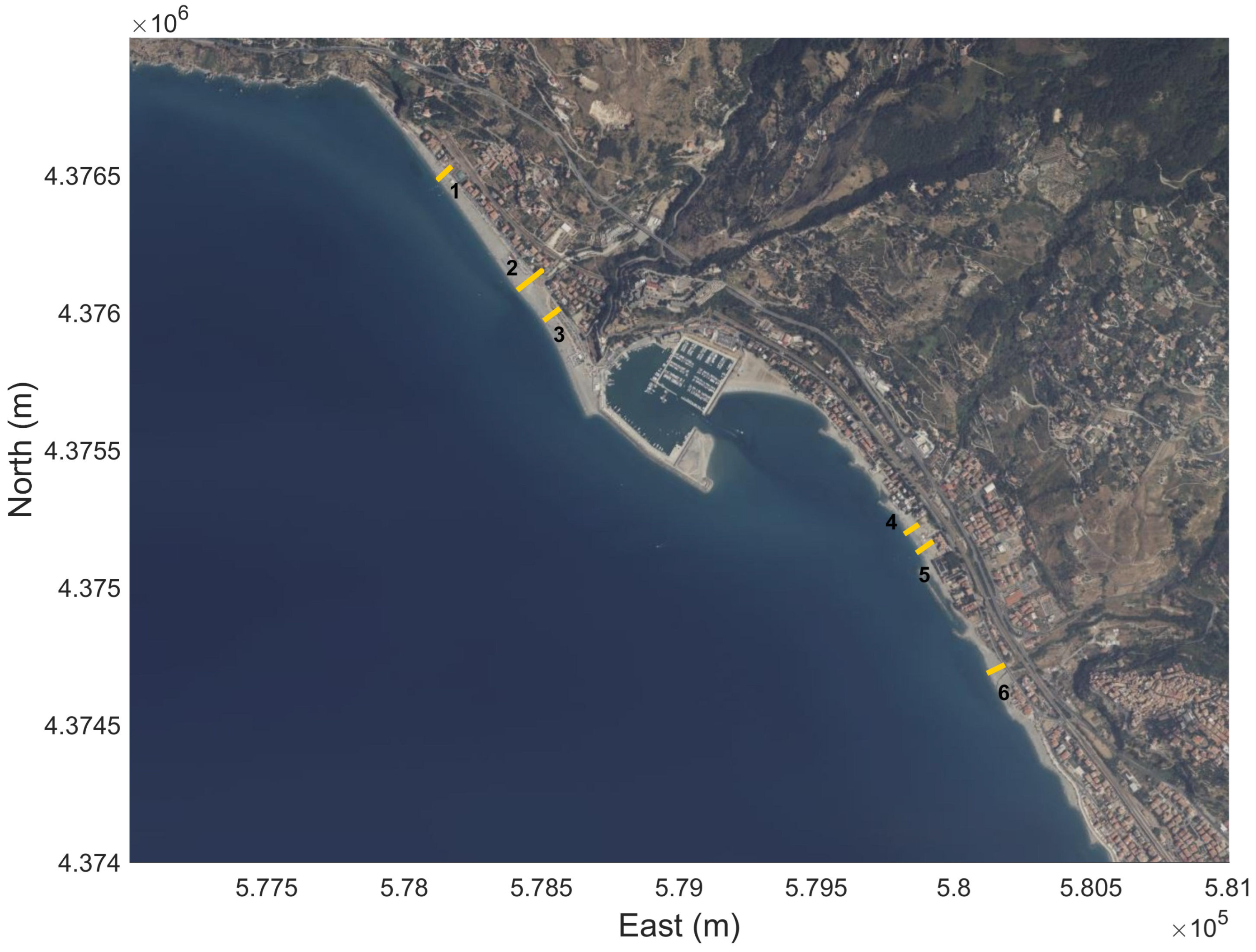
A local-scale quantification of the flooding mitigation effects induced by the presence of REWEC1 devices operating in no-air and fixed-air modes was finally carried out by analyzing wave set-up and run-up. To this end, a set of numerical gauges was placed along selected coastal transects using the XBeach model. Three transects were selected North of the port of Cetraro (transects 1, 2, and 3) and three South of the port (transects 4, 5, and 6), as shown in
Figure 18.
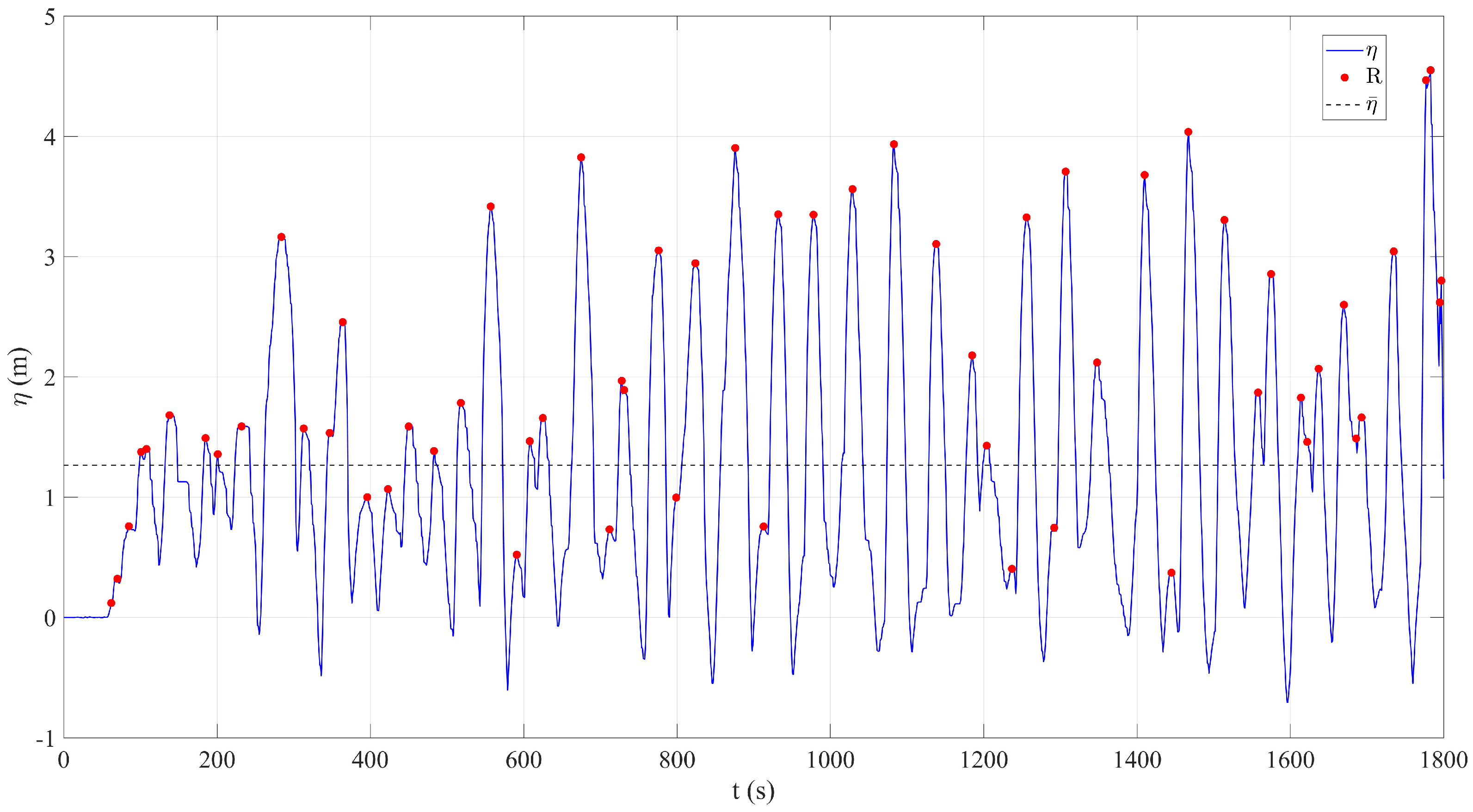
The time series of water levels
extracted at the numerical gauges from XBeach simulations were first corrected by removing the constant SLR contribution. The corrected time series were then preliminarily processed to remove high-frequency noise and isolated numerical spikes. A Hampel filter was applied, which detects outliers within a moving window based on deviations from the local median expressed as multiples of the median absolute deviation [
52]. The filtered time series were then used to compute the wave setup
as the temporal mean. To identify physically meaningful positive maxima corresponding to individual run-up events
R, three criteria were adopted. The first criterion concerns the minimum prominence, set equal to
, where
is the standard deviation of the filtered time series [
53]. The second criterion imposes a minimum duration of run-up events equal to
[
54], where
is obtained from spectral analysis of the filtered signal. The third criterion requires a minimum temporal separation between consecutive run-up events equal to
[
55]. An example of a water level time window for numerical gauge 1, including the identification of individual run-up events and the set-up level, is shown in
Figure 19.
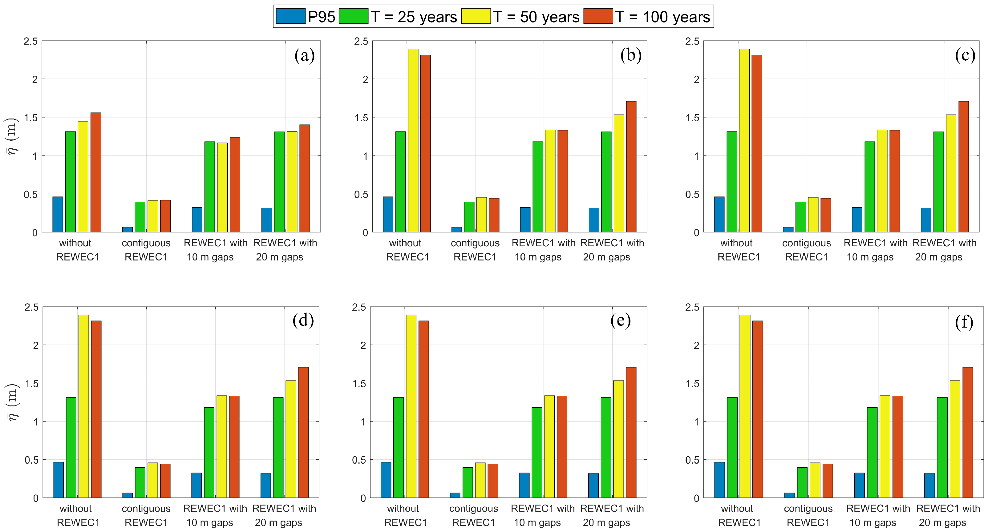
For the different spatial configurations, the computed set-up values
at the selected numerical gauges are reported in
Figure 20, referring to the P95 of
and the design waves with
T = 25, 50, and 100 years. The results exhibit variability depending on the local coastal morphology and on the characteristics of the incident wave field. In general, for all gauges, a progressive reduction in wave set-up is observed due to the presence of REWEC1 devices, from configurations with 20 m gaps to those with contiguous arrays, in agreement with the results obtained for maximum inundated areas and inland water penetrations. The difference in magnitude between the results obtained from the P95 of
and the different design waves is larger than in the cases of inundated areas and inland water penetration, as SLR was not considered in this analysis.
Table 3 reports the percentage reduction of wave set-up due to the presence of REWEC1 devices, expressed as the relative variation
, where
is the difference between set-up values in the absence and presence of REWEC1, and
is the set-up without REWEC1. The reductions exhibit spatial variability among numerical gauges due to the combined effects of local morphology and wave incidence. For contiguous REWEC1 arrays and for the configuration with 10 m gaps, the average set-up reduction is similar across all wave conditions, with mean values of 80.4% and 39.3%, respectively. For the configuration with 20 m gaps, the wave condition associated with the P95 of
leads to a mean set-up reduction of 31.6%, whereas the design wave conditions result in a mean set-up reduction of 18.4%.
From the individual run-up events
R recorded at each numerical gauge, the run-up exceeded by 2% of the events,
, corresponding to the 98th percentile of the
R distribution, was computed. This parameter is statistically robust and widely used in engineering applications.
Figure 21 shows the values of
at the selected gauges for the different spatial configurations, for the P95 of
and for the design waves with
T = 25, 50, and 100 years. The results for
further confirm the effectiveness of the REWEC1 devices in reducing the main hydrodynamic processes affecting the emerged coast.
Table 4 summarizes the percentage reductions of
induced by the presence of REWEC1 devices, expressed as the relative variation
, where
is the difference between
values in the absence and presence of REWEC1, and
is the run-up value without REWEC1. As for wave set-up, the reduction percentages are influenced by local coastal morphology and wave incidence. Overall, the average reduction of
is fairly similar of that observed for
(see
Table 3) for all wave conditions and REWEC1 configurations. The differences in mean reduction between
and
are less than 2%.
5.4. Uncertainty Analysis
An uncertainty analysis was conducted to evaluate the sensitivity of XBeach simulations to variations in the transmission coefficient
of the REWEC1 devices. In the SWAN simulations, the
values of REWEC1 for the selected spatial arrangements (contiguous, 10 m gaps, and 20 m gaps), obtained by the undisturbed wave field at a water depth of 10 m, were systematically varied by
to account for potential deviations arising from modeling assumptions, operational conditions, or inherent variability. Notably,
is a numerically derived parameter according to Filianoti and Piscopo [
21] and represents the principal hydraulic parameter for assessing the effectiveness of REWEC1 in reducing coastal flooding. In this analysis, the reflection coefficients
were kept fixed with respect to the reference values, as their values for the REWEC1 are consistently very low and their contribution to coastal flooding processes is negligible compared to transmission-driven effects.
The analysis focused on the worst-case scenario, corresponding to the design wave with
T = 100 years combined with RCP8.5 SLR. In this context, the REWEC1 units operated in no-air mode. The evaluation metrics were the maximum inundated areas and the maximum inland water penetration lengths. Comparing simulations with perturbed
values to the previous baseline results allowed for the quantification of uncertainty and the assessment of model robustness. This approach aligns with previous studies on uncertainty and sensitivity analysis in coastal hydrodynamic modeling (e.g., [
56]), underscoring the importance of accounting for parameter variability when evaluating extreme events.
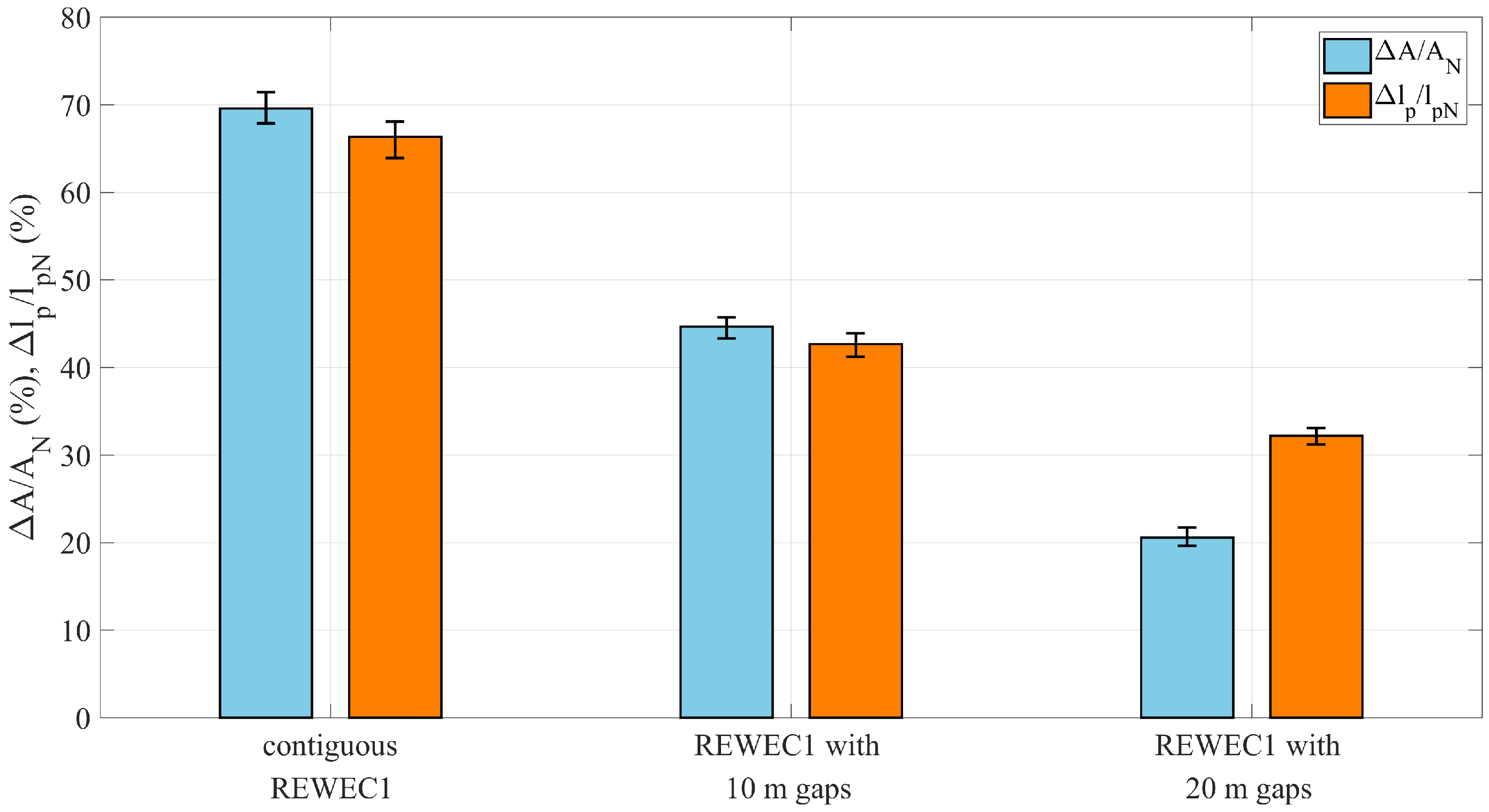
Based on the variability of the wave parameters at a water depth of 10 m for the selected design wave, ranges between 0.171 and 0.174 when the coefficient is reduced by 15%, and between 0.231 and 0.236 when it is increased by 15%. The disturbed wave field behind the REWEC1 at d = 7 m, obtained from SWAN simulations for different spatial configurations, was used as input, together with RCP8.5 SLR, for the subsequent XBeach simulations.
To analyze the sensitivity of coastal flooding to variations in the wave transmission coefficient
of the REWEC1 devices, two indicators were selected: the maximum inundated area and the maximum inland water penetration length. For the adopted spatial configurations (contiguous arrays, arrays with 10 m gaps, and arrays with 20 m gaps),
Figure 22 shows the relative reductions of flooding indicators
and
obtained using the reference
values and those derived by perturbing this parameter by
. Error bars are used to visualize the resulting variability, providing a quantitative representation of the potential range of outcomes under the selected extreme meteo-marine condition. The variability in
and
is generally small across all configurations, decreasing from approximately 4% for contiguous REWEC1 arrays to about 2% for arrays with 20 m gaps. Lower reductions in flooding indicators are observed for higher
values, while higher reductions correspond to lower
values. A slightly larger variability is noted for cases with higher
values, particularly in the contiguous configuration, highlighting the increased sensitivity of closely spaced arrays to changes in hydraulic performance. Overall, these results demonstrate that the selected
variation in
induces only minor changes in the predicted inundation patterns, regardless of the spatial configuration. This confirms the robustness and consistency of the trends reported in
Section 5.3, and supports the reliability of the REWEC1 performance assessment even under moderate uncertainties in the transmission coefficient.
5.5. Comparison with Rubble-Mound Breakwaters
In this Section, a comparison between REWEC1 and traditional submerged rubble-mound breakwaters in reducing coastal flooding was performed. The analysis considered the most extreme meteo-marine condition, i.e., the design wave with years combined with RCP8.5 SLR, across all spatial configurations (contiguous barriers, barriers with 10 m gaps, and barriers with 20 m gaps) operating in no-air mode.
The submerged rubble-mound breakwaters were placed at the same water depth ( m) and with the same height and length as the REWEC1 devices. They were composed of natural stones with a canonical seaward slope (tan() = 0.5) and an armour layer with a mean diameter of 2 m, ensuring stability under the applied wave forcing. To provide a consistent comparison, the hydraulic behaviour of the submerged rubble-mound breakwaters was modelled using transmission and reflection coefficients that depend solely on the incident wave conditions. Similar to REWEC1, SLR effects were not explicitly included in the coefficient formulation but were incorporated as a shift in the mean water level for the coastal flooding simulations.
The hydraulic characteristics adopted in SWAN simulations, in terms of
and
, were derived from various experimental-based formulas for low-crested rubble-mound breakwaters. For
, the semi-empirical equations developed by d’Angremond [
57], Seabrook and Hall [
58], and Briganti et al. [
59] were applied, which are valid within the range of the considered wave and geometrical conditions. Considering the variability of the incident wave parameters at
d = 10 m, the resulting
values obtained from the aforementioned formulas were averaged, yielding values between 0.364 and 0.397 depending on the specific location of the rubble mound breakwater and the local wave conditions. Similarly,
was derived by averaging the results from semi-empirical formulas by Seelig and Ahrens [
60], Ahrens [
61], and Zanuttigh and van der Meer [
62], resulting in values ranging from 0.260 to 0.278.
The wave field behind the rubble-mound breakwaters for all spatial configurations at a water depth of 7 m, induced by the
T = 100 year design wave and obtained from SWAN, was used as input for the XBeach simulations of coastal flooding, also accounting for RCP8.5 SLR. The resulting maximum flooded areas and maximum inland water penetration lengths were then compared with those obtained for the REWEC1 devices. In the comparison between REWEC1 and conventional rubble-mound breakwaters, the evaluation of flooding indicators for REWEC1 explicitly accounts for the uncertainty associated with a ±15% variation in the transmission coefficient
. This level of uncertainty is not considered for rubble-mound breakwaters, whose hydraulic performance is derived from well-established empirical relationships based on extensive experimental studies. The relative reductions in the flooding indicators
and
were evaluated by comparing REWEC1 and rubble-mound breakwaters for different spatial configurations. The indicators were computed by defining
and
as the differences between the maximum inundated area and maximum inland water penetration length in the presence of rubble-mound breakwaters and those obtained with REWEC1, respectively, while
and
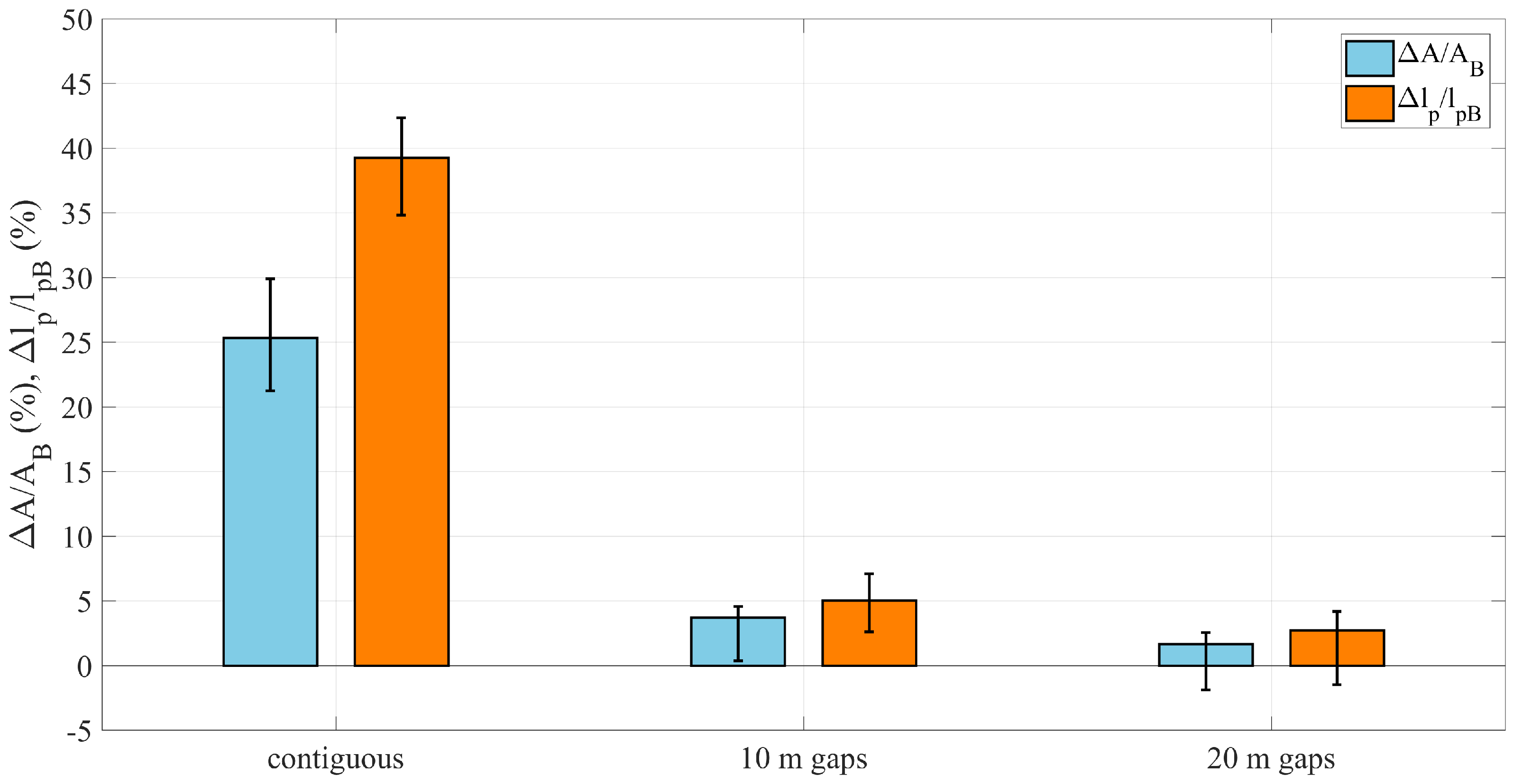
denote the corresponding values associated with the rubble-mound breakwaters. This formulation allows a direct assessment of the relative performance of REWEC1 in reducing coastal flooding with respect to conventional submerged breakwaters. The resulting relative reductions are shown in
Figure 23. For the contiguous arrangement, consistently positive values of
and, in particular, of
are observed, indicating a superior performance of REWEC1 units in mitigating coastal flooding with respect to rubble-mound breakwaters. Conversely, for the configurations with 10 m and 20 m gaps, the values of
and
are small and, in some cases, negative, suggesting that the flooding reduction capability of REWEC1 is comparable to that of conventional rubble-mound breakwaters when spatial discontinuities are introduced.