A Regional-Scale Early Warning System for Rainfall-Induced Shallow Landslides Based on the Outputs of a Physically Based Model: Application to Cili County, China

Abstract

This paper presents a new method for a regional-scale rainfall-induced landslide early warning system (LEWS) based on the outputs of the “Fast Shallow Landslide Assessment Model” (FSLAM), a physically based model used to compute slope stability at a regional scale. The LEWS combines landslide susceptibility and rainfall thresholds to depict the areas that are prone to slope failures and issues qualitative warnings over the study area. Both the susceptibility map and the rainfall thresholds were obtained based on the outputs from running FSLAM with 25 different rainfall scenarios. The final output of the LEWS is a slope-unit-based map. The LEWS was implemented for Cili County, Hunan Province, China, and tested for the year 2020. The warning level stayed “Low” during most of the year. High warnings were issued during the summer and were either due to intense rainfall events or abundant long-duration precipitation. The LEWS was able to issue appropriate warnings corresponding to the time and location of three known landslides that occurred in the study area in 2020. Although long-term validation with more landslide data and improved geotechnical data is needed to reduce the LEWS uncertainties, this approach is promising and could support authorities managing landslide risk.

1. Introduction

Landslides are a common natural hazard that occur in mountainous regions worldwide. Such hazardous events often impact infrastructure, buildings, and society, causing significant damage and socio-economic losses worldwide [1,2,3]. With climate change, extreme rainfall events that usually trigger landslides are expected to increase in many areas [4,5,6,7]. Building reliable landslide early warning systems (LEWSs) is key to reducing the risk by diminishing the exposure to such hazards [8].

To date, LEWSs have been developed and implemented at the local scale [9] and at the regional scale [10] in multiple areas of the world. Regional-scale LEWSs generally combine information from susceptibility maps to identify areas where landslides might initiate and determine if rainfall events can trigger landslides through rainfall thresholds [11,12,13,14,15,16]. Both the susceptibility maps and the rainfall thresholds are usually derived using empirical approaches to establish the relationship between the explanatory variables and historical landslide events. More recently, machine learning approaches have also been implemented in LEWSs [17,18,19]. Although these approaches are simple, they do not explicitly describe the mechanical and hydrological processes leading to slope failure.

Alternatively, slope stability physically based models [20,21,22,23,24] provide a more realistic description of the processes leading to landslides, and they have been adopted in local-scale LEWSs [25,26]. However, their implementation for regional-scale LEWS applications is challenging because of the limited availability of geotechnical data and the typically high computational demands of physically based models, which often require long computational times over large regions.

Recent developments have enabled physically based models to account for uncertainties in input geotechnical parameters [24,27,28,29]. Additionally, the continuous improvements in computational resources make the application of physically based models over larger areas increasingly feasible [30].

The main objective of this study is to develop a regional-scale LEWS method to compute rainfall-induced landslide warnings that benefits from physically based slope stability models. The aim is to establish a fast, simple, modular, and scalable framework that can be adapted for operational use in different regions to issue warnings over slope units. To achieve this, the following specific goals are defined: (i) obtain landslide susceptibility from the outputs of a physically based model, (ii) establish a methodology to objectively transform the outputs of a physically based landslide susceptibility model from pixels to slope units, and (iii) derive rainfall thresholds from the outputs of a physically based slope stability model. Cili County in the Province of Hunan, China, is used as a test site.

2. Description of the Study Area

2.1. Geographic, Geomorphological, and Climate Setting

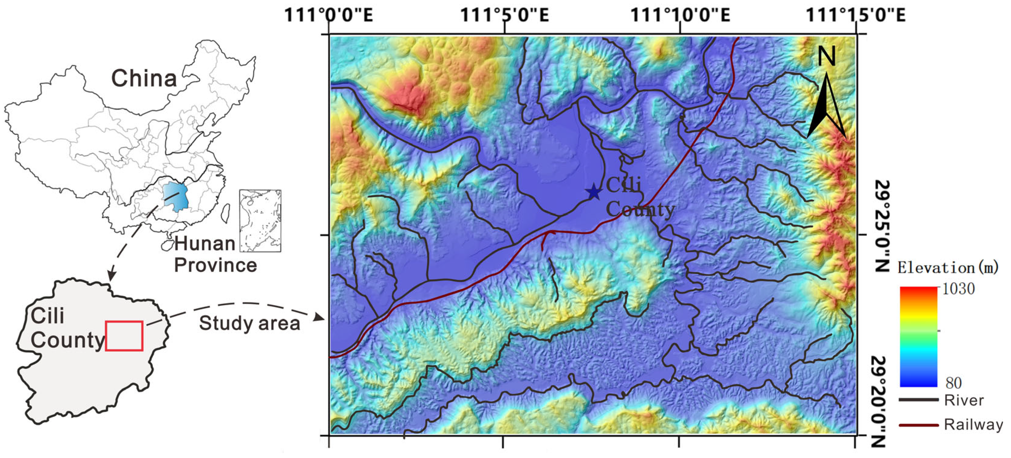
Part of Cili County, Hunan Province, located in southern China, was selected for the development of the physically based LEWS (Figure 1). The selected region has an area of approximately 445.9 km². The elevation of the region ranges from 80 m a.s.l to 1030 m a.s.l. From a geomorphological perspective, the region lies in the transition zone between the Wuling Mountains and the Xiangxi Mountains and the lakeside plain. The Lishui River, a tributary of the Yangtze River, drains through the central part of the study area.

The climate of the study area can be classified as mid-subtropical monsoon humid, with abundant rainfall and a long rainy season. According to the rainfall data from the Cili County Meteorological Bureau, the average annual rainfall in this area is 1376.9 mm. The abundant rainfall and mountainous terrain in the region provide the conditions for a large number of rainfall-induced landslides.

2.2. Landslide Inventory Data

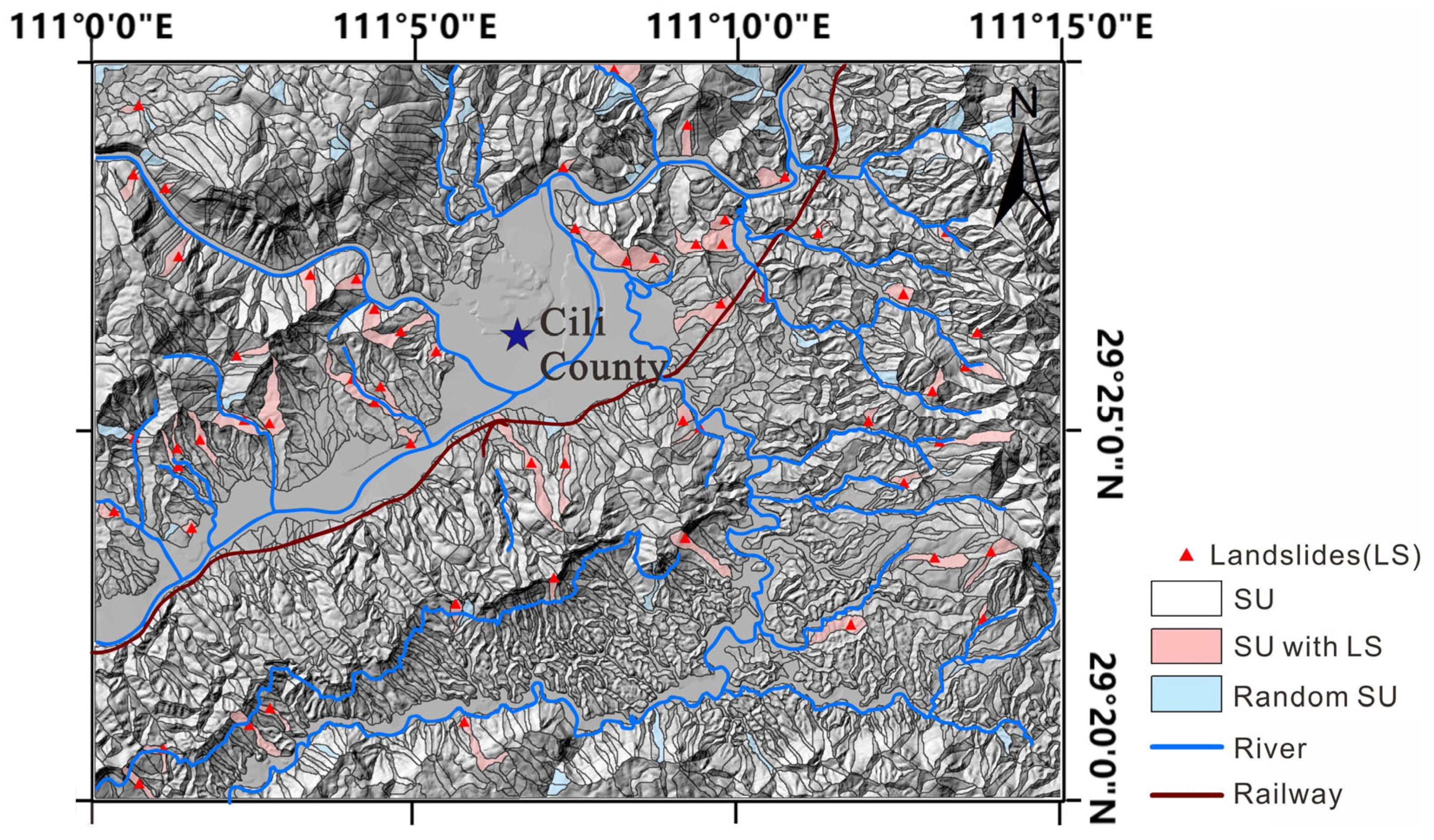
The landslide inventory (Figure 2) was provided by the China Geological Survey (CGS). It is based on data collected through field investigations over the past few years. The inventory contains 59 landslides that occurred in soil and that were triggered between 1987 and 2011.

Among the landslides in the inventory, 18 occurred in areas where the bedrock consists of argillaceous siltstone and sandy shale layers. Nine landslides were triggered in areas underlined by siltstones and sandy shales, and nine landslides occurred in areas where the bedrock consists of conglomerates with interbedded argillaceous siltstones. Finally, five landslides occurred in areas where the bedrock consists of interbedded sandstones and siltstones.

The landslides in the inventory generally occurred in the rainy season from June to August. In most cases, the landslides in the inventory were located in rather flat areas, with slope angles of less than 10°, where shallow landslides and debris flows generally do not occur. To deal with the spatial uncertainty in the landslide inventory, the locations of the landslides in the inventory were manually adjusted within a buffer of 50 m with the aid of topographic maps and aerial photos. All these 59 landslides were used to calibrate the physically based model used to establish the LEWS presented in this paper (

Table 1. Landslide inventory datasets used in this study.

Inventory Name	Time Period	Number of Landslides	Number of SUs with Landslides
Calibration	1987–2011	59	59
Verification	2020	3	3

). Additionally, the verification inventory was built with three additional landslides that affected infrastructure or buildings that occurred in 2020 (Table 1).

2.3. Other Available GIS Datasets

For this study, we used a 10 m resolution digital elevation model (DEM) provided by the China Geological Survey. The DEM was used as an input for the physically based slope stability calculations.

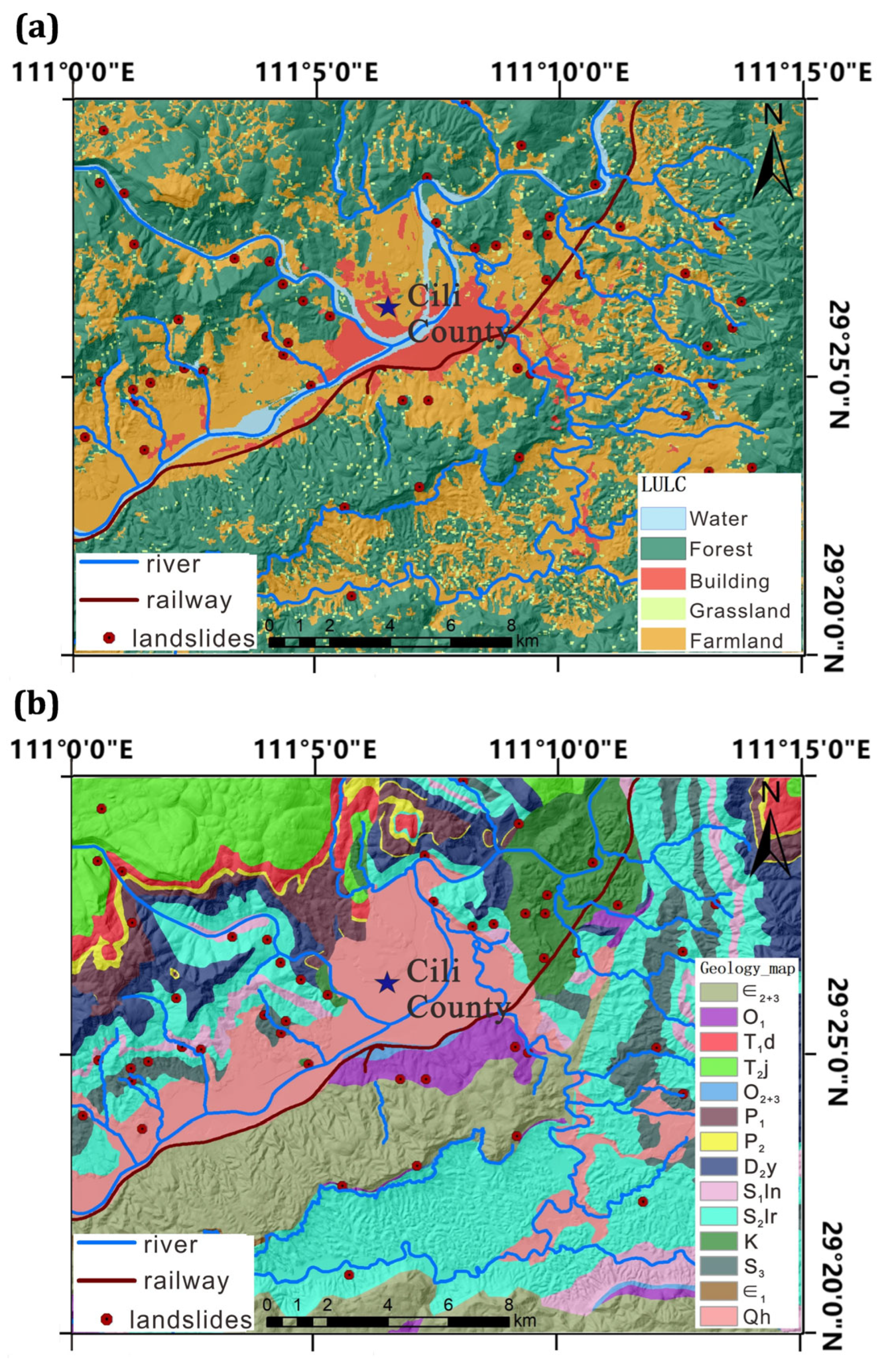
The land use and land cover (LULC) map from the public data of the Global Land Cover with Fine Classification System at 30 m in 2020 (GLC_FCS30-2020 [31]) of the Institute of Aerospace Information Innovation, Chinese Academy of Sciences, was used for the work presented in this paper. The study area was originally covered by 23 LULC classes, which were reclassified into 5 LULC types corresponding to water, forests, buildings, grasslands, and farmland (Figure 3a and

Table 2. Estimated root cohesion values (C_r) and curve numbers (CN) for the four LULC classes in the study area. These values were obtained during the calibration phase. CN-A, B, C, and D are the CN values for each hydrologic soil group (HSG).

LULC Class	Cr Min/Max (kPa)	CN-A (-)	CN-B (-)	CN-C (-)	CN-D (-)
Water	999/999	100	100	100	100
Forest	0/6	39	50	65	70
Buildings	0/0	81	88	91	93
Grassland	0/4	49	61	74	80
Farmland	0/2	30	39	49	58

).

There is no existing geotechnical soil map covering the study area. Only maps containing information on the bedrock lithology on the geological map at a scale 1:50,000, provided by the China Geological Survey are available. Converting a geological map into a soil map is challenging. Here, we assumed that surface soil mainly results from the weathering of in situ rock masses. The geological map from the China Geological Survey was reclassified into 14 lithology classes according to available descriptions (Figure 3b and

Table 3. Estimated values for the geotechnical parameters and hydrologic soil group (HSG) for each lithology class. These values were obtained during the calibration phase.

Code	Lithology Class	φ Min/Max (°)	Cs Min/Max (kPa)	z (m)	K (m/s)	N (-)	ρs (kg/m3)	HSG (-)
∈2+3	Dolomite	30/35	1/5	1.5	1 × 10−5	0.3	2000	B
O1	Limestone	25/35	0/4	2	1 × 10−5	0.3	2000	B
T1d	Limestone and dolomite	30/40	1/5	1.5	1 × 10−5	0.3	2000	B
T2j	Breccia-limestone	30/40	0/4	2	1 × 10−5	0.3	2000	B
O2+3	Argillaceous limestone and shale	25/30	1/4	3	1 × 10−6	0.35	2000	C
P1	Limestone and carbonaceous shale	25/35	0/4	2	1 × 10−6	0.3	2000	C
P2	Marl and siliceous rock	25/30	1/4	3	1 × 10−5	0.3	2000	B
D2y	Quarzitic sandstone	35/45	1/5	3	1 × 10−4	0.4	2000	A
S1ln	Sandstone and siltstone	30/35	0/4	2.5	1 × 10−4	0.4	2000	A
S2lr	Argillaceous siltstone	30/35	0/4	3	1 × 10−5	0.35	2000	A
K	Conglomerate and siltstone	25/30	0/3	2.5	1 × 10−5	0.35	2000	A
S3	Siltstone and sandy shale	25/30	0/3	2	1 × 10−6	0.4	2000	B
∈1	Slate and shale	20/35	0/5	2	1 × 10−5	0.3	2000	C
Qh	Sandy clay	25/35	1/3	3	1 × 10−5	0.35	2000	C

).

2.4. Rainfall Data

The study area is small and lacks rain gauges with long-term comprehensive observational data. Therefore, gridded rainfall data was used to analyze the rainfall conditions leading to landslide events in the study area from the year 1979 to 2018.

The rainfall data selected for this study was sourced from the China Meteorological Forcing Dataset (CMFD) [32], which offers a temporal resolution of 3 h and a spatial resolution of 0.1° × 0.1°. The geographical extent of the study area spans four rainfall grid cells (Figure 4), with the center at points p1, p2, p3, and p4. The comparison of the daily rainfall accumulation time series from the four adjacent grid cells showed that, in general, the differences in daily rainfall are limited. The average daily rainfall from June to August of the four grid cells is approximately 0.8 mm/day.

3. Methods

3.1. General LEWS Methodology

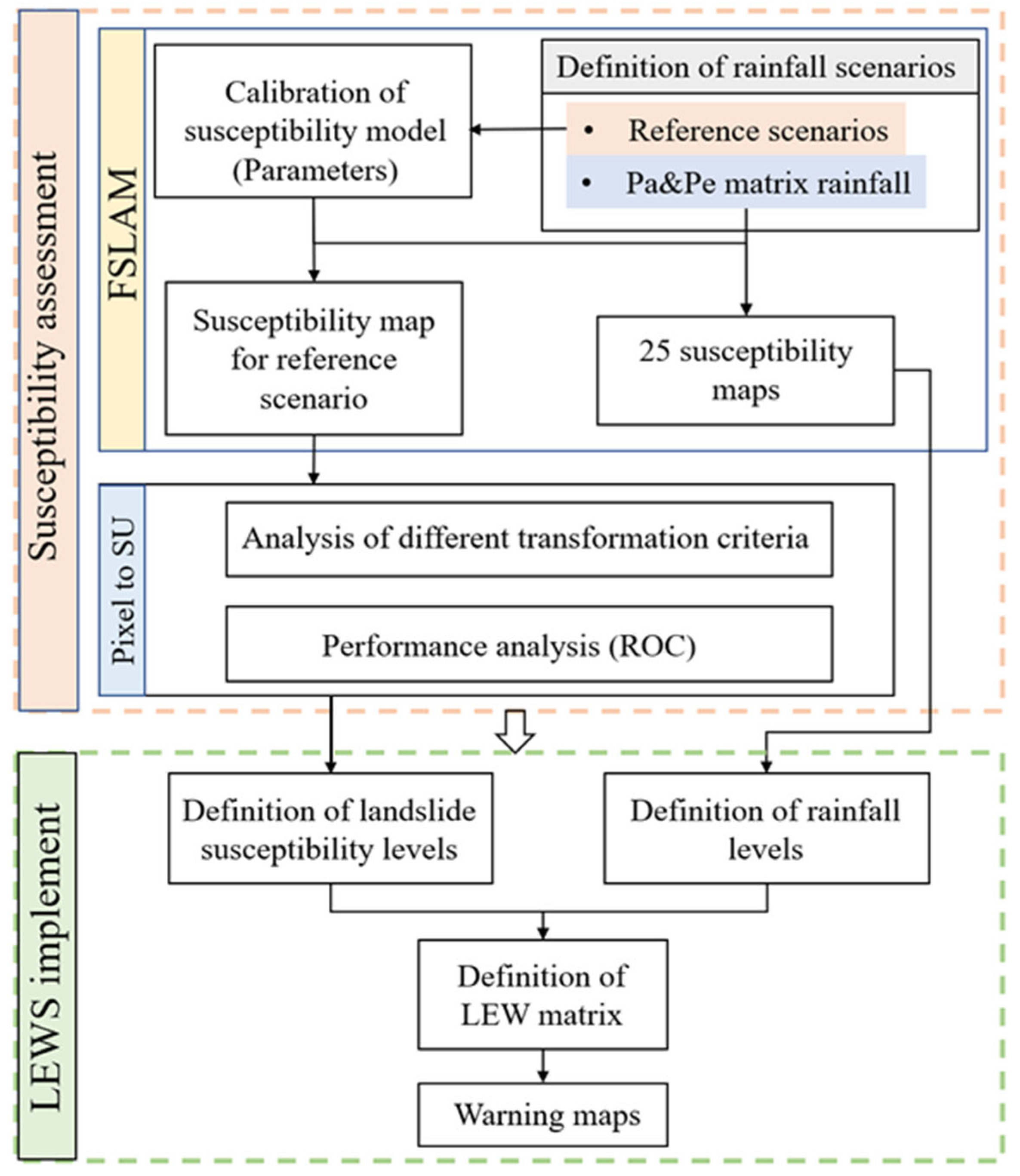
The LEWS adopts a physically based approach relying on outputs from FSLAM, a physically based model to assess slope stability at a regional scale. The FSLAM model is described in detail in Section 3.2. Figure 5 shows the flowchart of the general methodology of the LEWS.

To avoid the need to run FSLAM across the entire region every time new rainfall data becomes available, our approach combines information on susceptibility and rainfall hazard level (bottom panel in Figure 5). The susceptibility map was obtained by summarizing the probability of failure from FSLAM into slope units (top panel in Figure 5). Then, the SU-based probability-of-failure map was reclassified to distinguish four susceptibility classes: “Very Low”, “Low”, “Moderate”, and “High” (bottom panel in Figure 5).

Similarly, the rainfall thresholds were derived from FSLAM outputs. To achieve this, the physically based model was run using 25 rainfall scenarios resulting from different triggering-event rainfall and antecedent rainfall return periods (top panel in Figure 5). These thresholds are employed to classify the rainfall potential of triggering a landslide into four rainfall hazard level classes.

Finally, susceptibility and rainfall hazard level are combined using a warning matrix (Figure 6). The output of the LEWS is a map covering the study region that displays a qualitative warning level that can be either “Very Low”, “Low”, “Moderate”, or “High” for each slope unit.

3.2. Description of FSLAM

The different components of the LEWS were designed to benefit from the outputs of the Fast Shallow Landslide Assessment Model (FSLAM [24]). FSLAM is a physically based model used to compute slope stability over large regions (>100 km²) using high-resolution topographical information with a very short computational time. It applies the infinite slope theory and a simplified hydrological model to calculate slope stability.

With the infinite slope model, the factor of safety (FS) is computed as follows:

FS = C/(g·ρ_s·z·cosθ sinθ) + (1 − (h/z)·(ρ_w/ρ))·tanφ/tanθ

(1)

where $C$ is the cohesion, ${\rho }_{\mathrm{s}}$ is the density of the saturated soil, ${\rho }_{\mathrm{w}}$ is the density of water, $\theta$ is the terrain slope angle, $\phi$ is the soil internal friction angle, $h$ is the height of the water table, and $z$ is the soil depth. Both $h$ and $z$ are measured in the vertical direction. Cohesion is calculated as follows:

$$C=C_s+C_r$$

(2)

where $C_s$ is the effective soil cohesion, and $C_r$ is the apparent cohesion due to lateral root reinforcement.

To compute the water table, FSLAM [33,34] incorporates both lateral flow and vertical flow mechanisms. The mid–long-term effects of rainfall on the water table ($h_a$) associated with the antecedent rainfall ($P_a$) are characterized by lateral flow (q_a). The short-term influence of rainfall on the water table (h_e) related to a specific rainfall event (P_e) is characterized by fast vertical infiltration (q_e). The position of the water table is obtained as follows:

h = h_a + h_e

(3)

Over mid- and long-term timescales, antecedent rainfall (P_a) contributes to groundwater recharge (q_a), leading to quasi-steady groundwater level (h_a). Recharge represents the effective infiltration of precipitation after accounting for runoff and evapotranspiration. Since FSLAM does not include water balance algorithms, P_a represents the long-term effective infiltration and is expressed in mm/day.

As proposed by [20], h_a is computed as follows:

h_a = (a/b)·q_a/(K·sinθ cosθ)·(ρ_w/ρ_s)

(4)

where a is the drainage area, b is the cell size, K is the soil saturated hydraulic conductivity, and q_a is the effective antecedent water recharge due to the antecedent rainfall (P_a) [24].

The variation in the groundwater table due to the fast infiltration of the event rainfall is calculated as:

h_e = q_e/n

(5)

n is the soil porosity and q_e is the rainfall event infiltration, which is computed as proposed by the SCS-CN model [35]. This model was originally developed to compute the surface runoff associated with a rainfall event, but to achieve this, the infiltration is computed implicitly. Using the SCS-CN model, the infiltration is computed with the following equation:

q_e = P_e − [P_e − (5080/CN − 51)]²/(P_e + 4(5080/CN − 51))

(6)

where CN is the curve number, an adimensional empirical parameter ranging from 0 to 100 used in the SCS-CN model to predict direct runoff or infiltration from rainfall excess [35]. Higher CNs imply lower infiltration.

Finally, for the work presented in this paper, the soil cohesion, root cohesion, and the friction angle are incorporated as stochastic parameters [24]. Therefore, FSLAMs output consists of a map showing the probability of failure (PoF) ranging from 0 to 1 for each of the grid cells over the area where the model was run [24].

The values of the required geotechnical input parameters corresponding to the different lithology and LULC classes were obtained through parameter inversion calibration (Table 2 and Table 3) employing landslide data from the calibration inventory. To avoid failure in water areas, a very high root cohesion value is given. The selected soil parameters reasonably fit with the literature data. In addition, for each lithology class, the soil hydrologic group (HSG) [36] is provided (Table 3).

We implemented FSLAM using representative rainfall scenarios defined by return periods for both P_a and P_e. In the study area, landslides typically occur during June, July, and August, which coincide with the rainy season. Therefore, for P_a, we characterized the data by the daily average rainfall recorded during these three months from 1979 to 2018. For P_e, we used 24 h rainfall accumulations during the same period. Then, the return periods of 10, 20, 50, 100, and 200 years for both P_a and P_e were calculated using a Gumbel distribution (

Table 4. Estimated antecedent rainfall (P_a) and event rainfall (P_e) amounts corresponding to the 10, 20-, 50-, 100-, and 200-year return periods.

Return Period
	10 Years	20 Years	50 Years	100 Years	200 Years
Pa (mm/day)	1.18	1.33	1.52	1.67	1.82
Pe (mm)	150	171	198	219	240

). This methodology is widely used to simulate extreme rainfall events that can trigger landslides.

4. Results

4.1. Transformation from Pixels to Slope Units

For the ease of visualization during operational purposes, the LEWS uses slope-unit polygons to compute warnings. The following paragraphs describe the method used to objectively convert the pixel-based outputs from FSLAM into an SU-based map. Additionally, they describe how the thresholds for classifying the SU-based PoF map into four susceptibility classes were determined. To obtain the initial susceptibility map, FSLAM was run with the Pa and Pe corresponding to a 10-year return period to obtain a pixel-based map showing the PoF over the study area (Figure 7a). This combination of return periods was chosen to reflect commonly occurring rainfall conditions in the study area.

The study area was divided into slope units (SUs) employing the r.slopeunits method proposed by [37]. Figure 2 shows a map of the study area with the obtained SU polygons. To assign a single PoF value to each SU, four different methods were compared: (i) attributing the average PoF value af all the pixels within the SU, (ii) giving the PoF value corresponding to the 90th percentile from all the pixels within the SU, (iii) assigning the PoF corresponding to the 95th percentile of the pixels within the SU, and (iv) using the maximum PoF from the pixels within the SU.

The pixel-based outputs from FSLAM in Figure 7a show that the areas with the highest PoF are located in the northwest, northeast, and south of the study area. These areas correspond to mountainous regions characterized by steep slopes. In contrast, the PoF is generally near zero in the central part of the study area, where the valley floor is notably flat.

As expected, the areas where the SU-based maps display a higher PoF (Figure 7b–e) correspond to the areas where the pixel-based map has a higher PoF. From Figure 7, it can be noticed that the SU-based PoF maps do not cover the entire terrain. This is because flat areas located at the valley bottoms are excluded from the SU calculations in the r.slopeunits method.

Among the four tested approaches to summarize the pixel-based map into an SU-based map, the least conservative approach results from assigning the average PoF value to each SU (Figure 7b). With this method, a large number of SUs are assigned a PoF equal or lower to 0.5. As expected, the number of SUs with a PoF larger than 0.5 increases when using the 90th percentile method (Figure 7c) and is even higher with the 95th percentile method (Figure 7d). The most conservative approach is to assign the maximum PoF value, yielding an SU map with PoF values close to 1 across most of the study area (Figure 7e).

Both false positives and false negatives adversely impact the consistency of the model outputs. To address this, we chose to summarize the pixel-based PoF results using the 90th percentile of the pixels within each SU. This percentile was selected based on visual inspection of the PoF distributions in SUs with landslides and SUs without landslides, providing a compromise between over- and underestimation of susceptibility.

In order to transform the absolute PoF value inside SUs into four susceptibility levels, we tested several well-established classification methods available in most standard GIS software. These methods are summarized in

Table 5. Automatic classification methods integrated into GIS that were tested to obtain the PoF thresholds to classify the susceptibility map into “Very Low”, “Low”, “Moderate”, and “High”.

Methods	Principle
Equal interval	The range of PoF values is divided into equal-sized intervals.
Natural break	Thresholds are established when relatively large jumps appear in the PoF values determined by their variance.
Quantile	This is equivalent to assigning the same number of SUs in each class.
Standard deviation	Adds or subtracts a half standard deviation from the mean value of the PoF to define the susceptibility classes.

. We ultimately selected the standard deviation method. With this approach, PoF thresholds at 0.02, 0.50, and 0.98 define the limits between the “Very Low”, “Low”, “Moderate”, and “High” susceptibility classes. Figure 8 shows the classified susceptibility map of the study area.

4.2. Definition of Rainfall Thresholds

4.2.1. Definition of Rainfall Hazard

One of the assumptions of the proposed LEWS is that the geotechnical properties of the terrain remain constant over time; therefore, changes in the PoF result from variations in antecedent and event rainfall conditions. In this section, we establish a set of rainfall thresholds based on the outputs of the slope stability model.

To obtain the rainfall thresholds, FSLAM was run for the 25 possible combinations of antecedent rainfall scenarios corresponding to the average daily accumulations corresponding to 10-, 20-, 50-, 100-, and 200-year return periods and the event rainfall scenarios corresponding to the same return periods. Then, for each rainfall scenario, the FSLAM outputs were transformed from pixels to polygons. The rainfall hazard level (H_r) was defined as the percentage of SUs with a PoF greater than or equal to 0.5 for a given rainfall scenario.

Additionally, the PoF in dry conditions (i.e., P_e = 0 mm and P_a ≤ 1 mm/day) and the PoF for extreme rainfall situations (with very large return periods, for example, 1000 years) when the terrain becomes fully saturated were also computed, and the corresponding rainfall hazard levels were obtained.

The rainfall hazard level (H_r), antecedent rainfall (P_a), and event rainfall (P_e) for each of the simulated scenarios are represented in a 3D space defined by P_a, P_e, and H_r (Figure 9a). A non-linear function was fitted to the data relating H_r, P_a, and P_e, resulting in the following equation:

H_r = 0.364 + 0.001·P_e + 0.076·ln(P_a)

(7)

The coefficient of determination (R²) is 0.994. Rearranging the terms, the above expression can be written as:

H_r = 0.364 + P

(8)

where

P = 0.001·P_e + 0.076·ln(P_a)

(9)

This formulation is bounded by two limiting cases. The lower bound corresponds to the D_l value for dry conditions. Under these conditions, H_r is at its minimum, and H_r is equal to 0.28. The upper bound corresponds to the H_r value obtained for extreme rainfall situations, when the terrain is considered to be fully saturated. In such scenarios, almost all the area is unstable, and H_r equals 0.835.

Rainfall thresholds were finally established by defining iso-rainfall hazard level curves in the P_a, P_e, and H_r space to classify the rainfall hazard into the following four categories (Figure 9b): “Very Low” if H_r ≤ 0.42, “Low” if 0.42 < H_r ≤ 0.56, “Moderate” if 0.56 < H_r ≤ 0.70, and “High” if 0.70 < H_r.

4.2.2. Impact of Rainfall Hazard Level on Warnings

The LEWS was run using spatially uniform antecedent rainfall and event rainfall corresponding to the four rainfall hazard level scenarios (“Very Low”, “Low”, “Moderate”, and “High”), as defined in Section 4.2.1. The LEWS outputs corresponding to these four rainfall hazard level scenarios are shown in Figure 10.

As expected, when the rainfall hazard level is “Very Low” (Figure 10a), the warning level over most of the study area remains “Very Low”. In such a case, “Low” warnings are issued only over those SUs classified as having “High” susceptibility. As the rainfall hazard level increases, the number of SUs that display “Moderate” and “High” warnings also increases (Figure 10b–d). For extreme rainfall situations that lead to a “High” rainfall hazard level, the LEWS issues “Moderate” and “High” warnings over most of the study area (Figure 10d). “Low” warnings are then issued in the SUs classified as having “Very Low” susceptibility. This is reasonable, as during extreme rainfall events, landslides can be triggered in slopes that would generally be stable.

4.3. Analysis of the Performance of the LEWS

In this section, the performance of the LEWS presented in Section 3.1 is analyzed. To achieve this, the LEWS was run for the year 2020 using spatially uniform rainfall inputs. Due to the limited inventory data, the performance of the LEWS was analyzed (i) qualitatively in terms of the percentage of SUs where warnings were computed during the year and (ii) in terms of its ability to identify three specific landslide events that occurred during the year 2020, for which the location and date are known. For verification purposes, we considered that a warning was issued if the warning level was either “Moderate” or “High”.

4.3.1. Qualitative Evaluation of the LEWS Outputs

Figure 11 shows that no warnings were issued during most of the year. Moderate and High warning levels were issued only during the summer months (from June to August), coinciding with the time of the year when the largest rainfall amounts were recorded. The timing of the warnings aligns with the timing of past landslide events in the area, which are typically triggered during summer. It also corresponds with the period when the three recorded landslides in 2020 occurred.

While most warning days involved 25% of the slope units (SUs) in the study area, warnings were computed for approximately 50% of the SUs on 2 July 2020, when the Sipuncun landslide was triggered (Figure 11). From this 50%, 25% of the SUs issued a “Moderate” warning and 25% a “High” warning.

Warnings were issued in days with either (i) rainfall events with 24 h accumulations exceeding 150 mm (Figure 11) or (ii) days preceded by periods of substantial rain (Figure 11). Interestingly, on a few summer days with little-to-no recorded precipitation after periods with significant precipitation, “Moderate” warnings were computed over 25% of the SUs (Figure 11). These warnings were due to antecedent rainfall contributing to the build-up of pore pressures resulting in a “Moderate” rainfall hazard level in SUs classified as having “High” susceptibility.

4.3.2. Validation in Specific Sites

Due to the limited landslide inventory data collection, a quantitative evaluation of the LEWS performance was not possible. The LEWS outputs were analyzed in more detail for three specific SUs where landslides were reported in summer 2020. The three landslides initiated in SUs classified as having “High” susceptibility. The location of the three landslides is shown in Figure 10.

The Wuleishan landslide (landslide #1, Figure 12a) was triggered on 22 June 2020 in the northeast of the study area (Figure 10). It initiated in a slope covered by highly weathered sandstone–mudstone and mobilized approximately 500 m³ of sediment, blocking a scenic road that gives access to the Wulei Mountain.

The Sipuncun (landslide #2, Figure 12b) and Xinjiecun (landslide #3, Figure 12c) landslides occurred on 2 July 2020 and 8 July 2020 in two different SUs in the west of the study area (Figure 10). Landslide #2 was triggered in a nearly 2 m thick soil slope, with a length of about 150 m, a width of about 70 m, and a height of about 7 m, resulting in the destruction of three houses but no casualties. Landslide #3 was triggered in a slope covered by weathered sandstone–mudstone. The landslide caused significant impacts, damaging 31 houses, 230 m of road, 12.4 ha of farmland, and the electricity infrastructure, resulting in direct economic losses of CNY (Chinese Yuan) 10 million (Sichuan Province Geological Disaster Command Office and Sichuan Province Natural Resources Department 2021).

Figure 13 shows the rainfall and warning level time series at the SUs where the three landslides were observed. Since the LEWS was run using a uniform rainfall over the study area and the three SUs are classified as having “High” susceptibility, the warning level time series was identical at the three SUs.

In the three SUs where landslides occurred in 2020, the LEWS issued the first “Moderate” warning in response to a short but intense rainfall event that delivered approximately 180 mm in 24 h on 15 June 2020 (Figure 13). Following this rainfall event, the warning level rapidly decreased to “Low”. It increased again on 20 June as a consequence of a rainfall event that accumulated 40 mm. Although several rainfall events were recorded, the warning level remained “Moderate” for 10 days. On 2 July 2020, a rainfall event accumulated 200 mm in the study area, and the warning level rose to “High” (Figure 13). After this event, the warning level decreased to “Moderate,” and it remained so for several subsequent days. Some days had light rainfall; others were dry. Rainfall totals were low. The warning level dropped to “Low” around 24 July and briefly increased to “Moderate” on 26 July following a minor rainfall event (less than 20 mm). After this, the warning level remained “Low” for the rest of the summer.

The LEWS was capable of issuing warnings coinciding with the time and location of the observed landslides in the study area. The LEWS issued “Moderate” warnings at the specific locations and on the dates when landslides #1 and #3 were triggered (Figure 13) and a “High” warning at the time and location of landslide #2 (Figure 13). However, “Moderate” warnings were also issued at times when landslides were not reported.

Warning level changes are not only due to short-term 24 h rainfall accumulations but also due to the 30-day average antecedent rainfall. Following periods of high cumulative precipitation, the warning level remains “Moderate” for several days, even when daily rainfall is low or absent. This results in several days during which “Moderate” warnings are issued but no landslides are observed. Although only information about big landslides that caused damage is available, it is probable that most of these days with warnings might correspond to false positives.

5. Discussion and Conclusions

A new method for a regional-scale LEWS for rainfall-induced landslides has been developed and a prototype implemented in Cili County in the Province of Hunan, China. The LEWS has been designed to be used over large areas, with the aim of keeping computational costs small.

The LEWS is based on the outputs of FSLAM, a physically based model that computes slope stability at a regional scale. To avoid running the slope stability model across the entire region every time new rainfall data becomes available, our approach combines information on susceptibility and rainfall hazard level to issue warnings.

The static susceptibility map was obtained from the FSLAM pixel-based PoF output and transformed into an SU-based map. To achieve this, the 90th percentile of PoF was selected to aggregate pixel-level information for each SU. Then, the absolute 90th percentile PoF value in each SU was converted to one of the four susceptibility classes (Very Low, Low, Moderate, and High). To establish the PoF thresholds to define the four susceptibility classes, the standard deviation method in GIS was used. In conclusion, this method provides an objective way to transform the pixel outputs of a slope stability model into an SU-based susceptibility map that classifies terrain into four susceptibility classes.

Rainfall hazard was assessed using FSLAM outputs for 25 different rainfall scenarios, corresponding to all possible combinations of daily and monthly rainfall return periods. The outcome of the rainfall analysis is a non-linear function that expresses the rainfall hazard as a function of P_a and P_e. Additionally, we propose rainfall thresholds defined as iso-hazard curves in the P_a–P_e–H_r space, which allow us to classify a given rainfall scenario into one of four rainfall hazard levels. It is important to note that rainfall situations where P_a and P_e have return periods shorter than 10 years or longer than 200 years were not included in this analysis. Such conditions may become more frequent due to climate change. However, the presented thresholds can be adapted in the future to include a broader range of rainfall scenarios if necessary.

Finally, the susceptibility and rainfall hazard levels are combined to issue warnings using a warning matrix. The LEWS output is an SU-based map of the study area showing qualitative warnings. The LEWS output does not include probabilistic estimates or uncertainty bounds. The adopted warning matrix approach is similar to that implemented in existing regional-scale LEWS (e.g., [9,12,31,32,33]). However, such models usually employ empirical susceptibility maps and rainfall thresholds [38,39,40]. The presented LEWS relies on the outputs of a physically based model to obtain landslide susceptibility and the rainfall thresholds. This represents a step towards referring to the use of physically based landslide warning models, which allow for a better characterization of the mechanical and hydrological processes governing slope stability.

The LEWS was tested for 2020, which can be considered a relatively representative year regarding rainfall conditions in the study area. However, only three landslides were available for the validation, which is limited for robust quantitative assessments of the performance of the LEWS. Therefore, quantitative verification of the LEWS at a regional scale was not feasible. The performance of the LEWS was assessed qualitatively. The LEWS effectively issued warnings for three landslides that occurred during the summer of 2020. Warnings were computed during June and July, coinciding with the monsoon season. “Moderate” warnings were relatively frequent in 25% of the study area during these two months, especially in SUs classified as having “High” susceptibility. Since landslides are rare events, some of these warnings may represent false positives.

During 2020, warnings were given (i) on days with significant rainfall events and (ii) when cumulative precipitation over the preceding 30 days was abundant, even if little or no rainfall was recorded. These outcomes can be attributed to the fact that antecedent rainfall contributes to the build-up of pore pressures, bringing slopes closer to failure [41,42].

One factor that significantly influences LEWS performance is the quality of rainfall data [43]. Rainfall fields are highly non-stationary and have a large spatial variability. We assumed uniform rainfall across the study area, thereby neglecting the rainfall spatial variability. If these spatial variations were considered, we could expect differences in rainfall accumulation across the different SUs and thus distinct warning outputs. In the future, more reliable rainfall inputs like radar products could be employed to improve the spatial characterization of rainfall.

Another important challenge that directly affects the performance of the LEWS concerns the uncertainty in the soil geotechnical parameters. Here, lithology information, along with expert knowledge and information from historical landslide inventories, was used to calibrate FSLAM. However, these regional-scale inputs inevitably involve simplifications and assumptions that do not fully capture the small-scale spatial variability in soil properties, such as soil thickness, hydraulic conductivity, and shear strength. This can lead to uncertainty in the PoF estimates. In future, the input data could be improved by incorporating geotechnical data from field and lab tests.

The LEWS is explicitly designed for rainfall-triggered landslides in natural slopes and does not account for other triggering factors, such as earthquakes or anthropogenic activities, that might affect slope stability. However, the LEWS components can be updated in future if significant changes in LULC or terrain morphology occur.

The proposed LEWS framework is scalable and intended for application in other regions, provided that comparable rainfall, terrain, geology, and LULC data are available. However, a thorough quantitative verification of the performance of the LEWS, using a larger landslide inventory and spanning multiple years, should be conducted in the future to ensure the value of the LEWS outputs. This would also allow us to assess whether the LEWS adequately captures interannual variability in the rainfall patterns, antecedent moisture conditions, or extreme climate events. Finally, to enhance preparedness and timely emergency management, the LEWS should be run operationally using rainfall forecasts.

References

1. Froude, M.J.; Petley, D.N. Global Fatal Landslide Occurrence from 2004 to 2016. Nat. Hazards Earth Syst. Sci. 2018, 18, 2161–2181. [Google Scholar] [CrossRef]
2. Coalition for Disaster Resilient Infrastructure (CDRI). Global Infrastructure Resilience—Capturing the Resilience Dividend, 1st ed.; CDRI Secretariat: New Delhi, India, 2023. [Google Scholar]
3. Corominas, J.; Lantada, N.; Núñez-Andrés, M.A.; Mavrouli, O.C. Fatal Non-Seismic Rockfalls in Spain. Geoenvironmen. Disasters 2025, 12, 17. [Google Scholar] [CrossRef]
4. Corominas, J. Landslides and Climate. In Proceedings of the 8th International Symposium on Landslides, Cardiff, UK, 26–30 June 2000; pp. 1–33. [Google Scholar]
5. Gariano, S.L.; Guzzetti, F. Landslides in a Changing Climate. Earth-Sci. Rev. 2016, 162, 227–252. [Google Scholar] [CrossRef]
6. Kirschbaum, D.; Kapnick, S.B.; Stanley, T.; Pascale, S. Changes in Extreme Precipitation and Landslides Over High Mountain Asia. Geophys. Res. Lett. 2020, 47, e2019GL085347. [Google Scholar] [CrossRef]
7. Jacquemart, M.; Weber, S.; Chiarle, M.; Chmiel, M.; Cicoira, A.; Corona, C.; Eckert, N.; Gaume, J.; Giacona, F.; Hirschberg, J.; et al. Detecting the Impact of Climate Change on Alpine Mass Movements in Observational Records from the European Alps. Earth-Sci. Rev. 2024, 258, 104886. [Google Scholar] [CrossRef]
8. UNISDR. Sendai Framework for Disaster Risk Reduction 2015–2030; United Nations Office for Disaster Risk Reduction: Geneva, Switzerland, 2015. [Google Scholar]
9. Pecoraro, G.; Calvello, M.; Piciullo, L. Monitoring Strategies for Local Landslide Early Warning Systems. Landslides 2018, 16, 213–231. [Google Scholar] [CrossRef]
10. Guzzetti, F.; Gariano, S.L.; Peruccacci, S.; Brunetti, M.T.; Marchesini, I.; Rossi, M.; Melillo, M. Geographical Landslide Early Warning Systems. Earth-Sci. Rev. 2020, 200, 102973. [Google Scholar] [CrossRef]
11. Kirschbaum, D.B.; Stanley, T.; Simmons, J. A Dynamic Landslide Hazard Assessment System for Central America and Hispaniola. Nat. Hazards Earth Syst. Sci. 2015, 15, 2257–2272. [Google Scholar] [CrossRef]
12. Segoni, S.; Tofani, V.; Rosi, A.; Catani, F.; Casagli, N. Combination of Rainfall Thresholds and Susceptibility Maps for Dynamic Landslide Hazard Assessment at Regional Scale. Front. Earth Sci. 2018, 6, 85. [Google Scholar] [CrossRef]
13. Wei, L.-W.; Huang, C.-M.; Chen, H.; Lee, C.-T.; Chi, C.-C.; Chiu, C.-L. Adopting the I3R24 Rainfall Index and Landslide Susceptibility for the Establishment of an Early Warning Model for Rainfall-Induced Shallow Landslides. Nat. Hazards Earth Syst. Sci. 2018, 18, 1717–1733. [Google Scholar] [CrossRef]
14. Palau, R.M.; Hürlimann, M.; Berenguer, M.; Sempere-Torres, D. Influence of the Mapping Unit for Regional Landslide Early Warning Systems: Comparison between Pixels and Polygons in Catalonia (NE Spain). Landslides 2020, 17, 2067–2083. [Google Scholar] [CrossRef]
15. Khan, S.; Kirschbaum, D.B.; Stanley, T.A.; Amatya, P.M.; Emberson, R.A. Global Landslide Forecasting System for Hazard Assessment and Situational Awareness. Front. Earth Sci. 2022, 10, 878996. [Google Scholar] [CrossRef]
16. Shu, H.; He, J.; Zhang, F.; Zhang, M.; Ma, J.; Chen, Y.; Yang, S. Construction of Landslide Warning by Combining Rainfall Threshold and Landslide Susceptibility in the Gully Region of the Loess Plateau: A Case of Lanzhou City, China. J. Hydrol. 2024, 645, 132148. [Google Scholar] [CrossRef]
17. Stanley, T.A.; Kirschbaum, D.B.; Benz, G.; Emberson, R.A.; Amatya, P.M.; Medwedeff, W.; Clark, M.K. Data-Driven Landslide Nowcasting at the Global Scale. Front. Earth Sci. 2021, 9, 640043. [Google Scholar] [CrossRef]
18. Mondini, A.C.; Guzzetti, F.; Melillo, M. Deep Learning Forecast of Rainfall-Induced Shallow Landslides. Nat. Commun. 2023, 14, 2466. [Google Scholar] [CrossRef]
19. Nocentini, N.; Rosi, A.; Piciullo, L.; Liu, Z.; Segoni, S.; Fanti, R. Regional-Scale Spatiotemporal Landslide Probability Assessment through Machine Learning and Potential Applications for Operational Warning Systems: A Case Study in Kvam (Norway). Landslides 2024, 21, 2369–2387. [Google Scholar] [CrossRef]
20. Montgomery, D.R.; Dietrich, W.E. A Physically Based Model for the Topographic Control on Shallow Landsliding. Water Resour. Res. 1994, 30, 1153–1171. [Google Scholar] [CrossRef]
21. Pack, R.T.; Tarboton, D.G.; Goodwin, C.N. The SINMAP Approach to Terrain Stability Mapping. In Proceedings of the 8th Congress of the International Association of Engineering Geology, Vancouver, BC, Canada, 21–25 September 1998; A A Balkema: Vancouver, BC, Canada, 1998; Volume 2, pp. 1157–1166. [Google Scholar]
22. Baum, R.L.; Savage, W.Z.; Godt, J.W. TRIGRS—A Fortran Program for Transient Rainfall Infiltration and Grid-Based Regional Slope-Stability Analysis, Version 2.0; Open-File Report; U.S. Geological Survey: Reston, VA, USA, 2008; 75p. [Google Scholar]
23. Lehmann, P.; Or, D. Hydromechanical Triggering of Landslides: From Progressive Local Failures to Mass Release. Water Resour. Res. 2012, 48, W03535. [Google Scholar] [CrossRef]
24. Medina, V.; Hürlimann, M.; Guo, Z.; Lloret, A.; Vaunat, J. Fast Physically-Based Model for Rainfall-Induced Landslide Susceptibility Assessment at Regional Scale. CATENA 2021, 201, 105213. [Google Scholar] [CrossRef]
25. Piciullo, L.; Capobianco, V.; Heyerdahl, H. A First Step towards a IoT-Based Local Early Warning System for an Unsaturated Slope in Norway. Nat. Hazards 2022, 114, 3377–3407. [Google Scholar] [CrossRef]
26. Piciullo, L.; Abraham, M.T.; Drøsdal, I.N.; Paulsen, E.S. An Operational IoT-Based Slope Stability Forecast Using a Digital Twin. Environ. Model. Softw. 2025, 183, 106228. [Google Scholar] [CrossRef]
27. Zhang, S.; Zhao, L.; Delgado-Tellez, R.; Bao, H. A Physics-Based Probabilistic Forecasting Model for Rainfall-Induced Shallow Landslides at Regional Scale. Nat. Hazards Earth Syst. Sci. 2018, 18, 969–982. [Google Scholar] [CrossRef]
28. Cui, H.; Hürlimann, M.; Medina, V.; Ji, J. GIS-FSLAM-FORM: A QGIS Plugin for Fast Probabilistic Susceptibility Assessment of Rainfall-Induced Landslides at Regional Scale; Copernicus Meetings: Berlin/Heidelberg, Germany, 2023. [Google Scholar]
29. Cui, H.; Ji, J.; Hürlimann, M.; Medina, V. Probabilistic and Physically-Based Modelling of Rainfall-Induced Landslide Susceptibility Using Integrated GIS-FORM Algorithm. Landslides 2024, 21, 1461–1481. [Google Scholar] [CrossRef]
30. Lin, W.; Yin, K.; Wang, N.; Xu, Y.; Guo, Z.; Li, Y. Landslide Hazard Assessment of Rainfall-Induced Landslide Based on the CF-SINMAP Model: A Case Study from Wuling Mountain in Hunan Province, China. Nat. Hazards 2021, 106, 679–700. [Google Scholar] [CrossRef]
31. Zhang, X.; Liu, L.; Chen, X.; Gao, Y.; Xie, S.; Mi, J. GLC_FCS30: Global Land-Cover Product with Fine Classification System at 30 m Using Time-Series Landsat Imagery. Earth Syst. Sci. Data 2021, 13, 2753–2776. [Google Scholar] [CrossRef]
32. Yang, K.; He, J.; Tang, W.; Lu, H.; Qin, J.; Chen, Y.; Li, X. China Meteorological Forcing Dataset v1.6 (1979–2018); National Tibetan Plateau Data Center: Xining, China, 2025. [Google Scholar]
33. Abancó, C.; Asurza, F.A.; Medina, V.; Hürlimann, M.; Bennett, G.L. Modelling Antecedent Soil Hydrological Conditions to Improve the Prediction of Landslide Susceptibility in Typhoon-Prone Regions. Landslides 2024, 21, 1531–1547. [Google Scholar] [CrossRef]
34. Cui, H.; Medina, V.; Hürlimann, M.; Ji, J. Fast Physically-Based Probabilistic Modelling of Rainfall-Induced Shallow Landslide Susceptibility at the Regional Scale Considering Geotechnical Uncertainties and Different Hydrological Conditions. Comput. Geotech. 2024, 172, 106400. [Google Scholar] [CrossRef]
35. USDA. Urban Hydrology for Small Watersheds; National Resources Conservation Service: Washington, DC, USA, 1986. [Google Scholar]
36. USDA (United States Department of Agriculture). Part 630 Hydrology. National Engineering Handbook. Chapter 7 Hydrologic Soil Groups; USDA: Washington, DC, USA, 2007. [Google Scholar]
37. Alvioli, M.; Marchesini, I.; Reichenbach, P.; Rossi, M.; Ardizzone, F.; Fiorucci, F.; Guzzetti, F. Automatic Delineation of Geomorphological Slope Units with r.Slopeunits v1.0 and Their Optimization for Landslide Susceptibility Modeling. Geosci. Model Dev. 2016, 9, 3975–3991. [Google Scholar] [CrossRef]
38. Jakob, M.; Owen, T.; Simpson, T. A Regional Real-Time Debris-Flow Warning System for the District of North Vancouver, Canada. Landslides 2012, 9, 165–178. [Google Scholar] [CrossRef]
39. Krøgli, I.K.; Devoli, G.; Colleuille, H.; Boje, S.; Sund, M.; Engen, I.K. The Norwegian Forecasting and Warning Service for Rainfall- and Snowmelt-Induced Landslides. Nat. Hazards Earth Syst. Sci. 2018, 18, 1427–1450. [Google Scholar] [CrossRef]
40. Segoni, S.; Serengil, Y.; Aydin, F. A Prototype Landslide Early Warning System in Rize (Turkey): Analyzing Recent Impacts to Design a Safer Future. Landslides 2023, 20, 683–694. [Google Scholar] [CrossRef]
41. Terzaghi, K. Theoretical Soil Mechanics; John Wiley & Sons, Inc.: Hoboken, NJ, USA, 1943; ISBN 978-0-470-17276-6. [Google Scholar]
42. Bogaard, T.; Greco, R. Landslide Hydrology: From Hydrology to Pore Pressure. WIREs Water 2016, 3, 439–459. [Google Scholar] [CrossRef]
43. Marra, F.; Destro, E.; Nikolopoulos, E.I.; Zoccatelli, D.; Creutin, J.D.; Guzzetti, F.; Borga, M. Impact of Rainfall Spatial Aggregation on the Identification of Debris Flow Occurrence Thresholds. Hydrol. Earth Syst. Sci. 2017, 21, 4525–4532. [Google Scholar] [CrossRef]
Figure 1. General location and digital elevation map of the study area.
Water 18 00168 g001
Figure 2. Shaded relief overview map of the study area. Grey polygons represent the 2296 slope units (SUs) subdivision of the terrain (see Section 3 and Section 4). Red triangles indicate the location of landslides in the inventory that were used for the calibration of the physically based susceptibility map. Pink polygons highlight slope units containing landslides. Blue polygons denote the randomly selected slope units with no observed landslide observations.
Water 18 00168 g002
Figure 3. (a) LULC map of the study area; (b) lithological map of the study area (see Table 3 for abbreviations used in legend). The red dots represent the location of landslides in the calibration inventory.
Water 18 00168 g003
Figure 4. The left panel shows the rainfall data from the China Meteorological Forcing Dataset (CMFD) over mainland China for 30 January 2012. The extent of the study area is indicated by the red box, which is covered by four grid cells (p1, p2, p3, and p4). The right panel shows the average daily rainfall from June to August in the four pixels covering the study area.
Water 18 00168 g004
Figure 5. Flowchart illustrating the general methodology of the LEWS.
Water 18 00168 g005
Figure 6. Warning matrix used to compute the warnings. Rows represent the classified susceptibility; columns represent the rainfall hazard levels. “VL”, “L”, “M”, and “H” represent “Very Low”, “Low”, “Moderate”, and “High” warning levels.
Water 18 00168 g006
Figure 7. Transformation from pixel to slope units (SUs). (a) The original pixel-based PoF map obtained from FSLAM. Transformed SU-based maps obtained when assigning (b) the average PoF value from the pixels within each SU, (c) the PoF corresponding to the 90th percentile of all the pixels within each SU, (d) the PoF corresponding to the 95th percentile of all the pixels within each SU, and (e) the maximum PoF from the pixels within each SU.
Water 18 00168 g007
Figure 8. Classified susceptibility maps of the study area obtained applying the standard deviation method to obtain the boundaries within “Very Low”, “Low”, “Moderate”, and “High” susceptibility.
Water 18 00168 g008
Figure 9. Determination of rainfall hazard classes. (a) Non-linear curve fitted into the Pa, Pe, and rainfall hazard points (in red) resulting from running FSLAM with 25 different rainfall scenarios. (b) Schematic diagram representing the iso-rainfall hazard lines chosen to define the Very Low (VL), Low (L), Moderate (M), and High (H) rainfall hazard classes.
Water 18 00168 g009
Figure 10. Warning maps corresponding to (a) “Very Low”, (b) “Low”, (c) “Moderate”, and (d) “High” rainfall hazard level scenarios. The triangles with labels (1), (2), and (3) indicate the location of landslides #1, #2, and #3 of the validation inventory.
Water 18 00168 g010
Figure 11. Daily rainfall and warning level time series in 2020. The light-blue bars represent the 24 h rainfall accumulations. The red line represents the percentage of SUs with a “Moderate” or “High” warning level. The navy line represents the percentage of SUs with “High” warning. The dates when landslides were reported in the area are marked with black polygon markers.
Water 18 00168 g011
Figure 12. Landslides observed during summer 2020 that were used for the LEWS validation in specific sites. (a) Wuleishan landslide (landslide #1); (b) Sipuncun landslide (landslide #2), and (c) Xinjiecun landslide (landslide #3). The geographical location of the three landslides can be observed in Figure 10.
Water 18 00168 g012
Figure 13. Rainfall and warning level time series during the summer of 2020 at the location of the three observed landslides. The susceptibility at the location of the three landslides is “High”.
Water 18 00168 g013