Abstract
Effective flood management requires a comprehensive understanding of interactions between multiple flooding sources. This study investigates compound flooding in the Brisbane River Estuary (BRE), Australia, using the MIKE 21 hydrodynamic model to assess the combined effects of tidal and riverine processes on flood extent and water levels. Unlike conventional studies that evaluate these factors separately, this research quantifies the impact of boundary condition variations at the Moreton Bay entrance on flood modelling accuracy. The model was calibrated by adjusting Manning’s n, achieving a Nash–Sutcliffe efficiency (Ens) ranging from 0.84 to 0.95. Validation results show a 90% agreement between the simulated and observed 2011 flood extent. The findings highlight the critical role of tidal boundary conditions, as their exclusion led to a 0.62 m and 0.12 m reduction in flood levels at Jindalee and Brisbane City gauges, respectively. This study provides valuable insights for improving flood risk assessment, model accuracy, and decision-making in estuarine flood management.
1. Introduction
Flooding is a prevalent and most destructive catastrophe worldwide, which poses a severe threat to lives and properties [1,2,3]. Coastal flooding is likely to increase in the future [4] due to sea-level rise, increased storm surge, land subsidence, and urbanization [5,6,7]. Flooding caused a global economic loss of USD 70.1 billion between 2000–2015 [3], affecting 2.3 billion people [8]. It is anticipated that global flood losses will hit AUD 1.59 trillion per year in 2050 [9,10,11,12,13]. For instance, in South East Queensland (SEQ), Australia, the 2011 flood affected more than 2.5 million people and around 29,000 homes in the Brisbane River Valley [14,15]. The flooding led to 35 deaths and AUD 2.55 billion in economic loss [16]. Recent reports show that climate change is contributing to the frequency and intensity of such flood events, particularly in coastal Australia [17].
In coastal catchments, floods can be produced by runoff generated by a significant rainfall event [18] and a raised ocean level produced by a storm surge, or a combination of both. A storm surge is the rise of water level above the normal sea level along a coast due to reduced atmospheric pressure and/or strong coastal winds [19]. The storm surge influences may further increase when they coincide with riverine flooding [20], and the resulting combination leads to a compound flood event [21,22]. Compound flooding, defined as the interaction of two or more flood drivers (e.g., tidal, riverine, and pluvial), has garnered increasing attention. Recent research reviewed over 270 studies, identifying key gaps in coastal and estuarine compound flood modelling, including inconsistent terminology and a lack of coupled dynamic systems [23].
Tropical cyclones, some hundred kilometres north of Moreton Bay, cause high waves and storm surges inside Moreton Bay. These events usually do not produce storm winds within Moreton Bay; however, they can make big ocean swell waves. It has been recognized that the wave circumstances produced by far-away cyclones can cause a deviation in Moreton Bay water levels [24]. The mixture of storm surge and normal tide is known as a storm tide, and disastrous impacts occur when the storm surge coincides with a high tide, intensifying flooding. As a result, the storm tide can influence areas further upstream in the estuary. Ongoing sea-level rise will increase river tailwater levels, particularly during storm surges, allowing surges to penetrate further inland. Initially, the two flooding drivers involved were managed individually in coastal flood management [25]. However, studies have shown that storm surge and extreme rainfall are statistically dependent, and their combined effects must be considered in coastal flood risk analysis [26,27,28]. To reduce adverse impacts, it is vital to employ integrated modelling frameworks that simulate compound flood scenarios, including future storm surge projections.
A notable example is Tropical Cyclone Alfred, which made landfall over the Moreton Bay Islands in March 2025. Although it weakened to a tropical low upon reaching the mainland between Brisbane and Maroochydore, Cyclone Alfred caused significant disruptions, including severe rainfall, damaging winds, and mass power outages affecting over 58,000 homes and businesses in Queensland. This event underscores the critical need to understand and manage the combined effects of storm surges and riverine flooding in the region, including those impacting southeast Queensland [17].
In the past, various researchers have given substantial efforts to simulate flood inundation in the coastal floodplain with different numerical modelling approaches [29,30]. Further, flood hydrodynamic modelling has significantly improved with advanced approaches including digital elevation models (DEMs). Flood modelling simulation accuracy mainly depends on the suitable discretization of the geometric domain and grid resolution of the DEM [3]. Recent modelling advances include dynamic coupling of riverine and tidal systems, high-resolution topographic inputs, and multi-model intercomparisons [31]. However, challenges remain in model convergence, uncertainty representation, and validation using historical compound flood datasets.
The literature review revealed that existing flood studies are conducted with and without considering the compound flood and future storm surge event effects [32]. For instance, Karim and Mimura [19] studied the influences of sea-level rise (SLR) on storm surge flooding in Western Bangladesh, and the hydrodynamic model simulation showed that for a storm surge under 0.3 m SLR, the flooded area would enlarge by 15.3% of the current flooded area. However, there is no systematic framework for considering compound floods from multiple sources for a specific case study.
More frequent flooding events in the Brisbane River Estuary (BRE) specify the need for a sustainable modelling approach to simulate the flood extent and propose measures to alleviate future flooding. To assess the flood hydrodynamics, BRE Australia was studied, which has been exposed to several flooding events over the past century, while it has experienced two destructive flooding events in the years 2011 and 2013 when a storm surge coincided with extreme riverine discharge in the BRE [33]. Earlier studies have utilized the 2D hydrodynamic model for Brisbane River flood modelling and coastal management [1,34]. However, the combined effect of riverine and storm surges was not considered, with the future effect of storm surges [22]. For flood assessment and inundation mapping, both temporal and spatial (flood depth and inundation extent) knowledge is required and can be applied in the flood risk analysis [1,35]. However, existing studies on the Brisbane River have used coarser-resolution geometric data, with 66.9% accuracy of flood modelling results, which leads to uncertainty and is less precise for coastal management [36]. Other studies used a combination of hydrological and hydraulic models for BRE flood extent assessment. However, these models require extensive input data, and further, they are restricted to government use and have limited access for research studies. The complexity of the Brisbane River area for flood forecasting, found by analysing the compound flooding risks and considering future storm surge scenarios, is still a significant and challenging study [37], which led to the development of the hydrodynamic model for BRE for flood inundation. This study improves on previous work by integrating fine-resolution meshes and a boundary-sensitive configuration using the MIKE 21 model. These additions help overcome limitations seen in prior Brisbane River studies. Novel elements include testing five mesh configurations to evaluate computational trade-offs and isolating boundary impacts in estuarine dynamics, which is rare in existing literature [23].
This study investigates the hydrodynamics of the Brisbane River Estuary (BRE) using the MIKE 21 hydrodynamic model to analyse flood extent under varying mesh resolutions. Unlike previous studies that often assess tidal or riverine flooding in isolation, this research explicitly examines the compound interactions between storm tides and fluvial flooding. Specifically, we assess how different boundary conditions at the Moreton Bay entrance influence modelled water levels and flood extents in the estuary.
The objectives of this study are threefold: (1) to develop a flood model for the Brisbane River Estuary and Moreton Bay using MIKE 21 that explicitly incorporates compound flooding dynamics; (2) to simulate and quantify the combined impacts of riverine flooding and tidal interactions on water levels; and (3) to evaluate the influence of future storm surges on flood extent and severity. Unlike conventional studies that primarily focus on either tidal or riverine contributions to flooding, our approach integrates both processes while examining the role of boundary conditions and mesh resolution in hydrodynamic modelling accuracy.
The findings of this study contribute to advancing flood modelling methodologies by demonstrating the significance of boundary conditions and grid resolution in accurately simulating compound flood events. This work provides valuable insights for flood risk assessment, helping policymakers and engineers develop more effective flood mitigation and management strategies tailored to estuarine environments.
The Flow Model of MIKE 21 is the basic hydrodynamic module. It provides the hydrodynamic basis for the computations of coastal hydraulics. It models the flows and variations of water levels in response to a range of forcing functions on floodplains, lakes, estuaries, and coastal areas. Many researchers have successfully used the MIKE 21 FM model to investigate the hydrodynamic process of a large river and coastal bay, like Dongting Lake, China [38]; the Poyang Lake, China [39,40]; the Brisbane River estuary [41]; Vembanad Lake, India [42]; Lake Alexandrina [43]; and Deer Creek in the City of Brentwood [44]. The MIKE 21 FM hydrodynamic module was used to simulate the depth-averaged flow features for the years 2006, 2011, and 2013 of the Brisbane River and Moreton Bay.
The paper is structured as follows: the case study area, the Brisbane River estuary (BRE), is described in Section 2. Section 3 explains the Brisbane flooding, the hydrodynamic model, the data requirements, and methods, including the mesh resolution effect and compound flooding in BRE. The results of the hydrodynamic model calibration and validation, along with mesh effects and compound flooding influence, are described and discussed in Section 4. Finally, conclusions are specified in Section 5.
2. Study Area
The Brisbane River and Moreton Bay are located on the southeast coast of Queensland, Australia (Figure 1). The lower part of the Brisbane River is termed the Brisbane River estuary (BRE). Moreton Bay is a semi-closed coastal water situated at the mouth of the Brisbane River. BRE and Moreton Bay experience semidiurnal tides with a tidal range of 2.5 m. The Brisbane River has the longest course in sub-tropical SEQ, having a length of 344 km, and has a catchment area of 13,600 kmP2 [45] to the Port Office Gauge, which is located in the heart of Brisbane City. The BRE is a micro-tidal estuary, with a mean spring and neap tidal range of 1.8 m and 1.0 m, respectively [46]. It has a tidal influence up to 80 km from the river mouth. The Oxley Creek and Bremer Rivers are major tributaries, which contribute to lower half catchment flows in BRE and join the estuary at 34 and 73 km, respectively, from the river mouth. Estuary depth varies, from 15 m at the river mouth to about 4 m above the Australian Height Datum (AHD) at the Bremer River junction at Moggill Point.
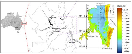
Figure 1.
Brisbane River catchment and Moreton Bay.
The catchment is manifold, joining rural and urban land, dams for flood mitigation, tidal impacts, and various tributaries, with the prospect of flooding. The river system itself contains the Brisbane River and numerous main tributaries. The Brisbane River has two dams situated in its upper catchment, both of which were constructed with the twin objective of flood alleviation and water supply to Brisbane City. Wivenhoe Dam regulates the flow of water in the upper part of the Brisbane River, which is approximately 150 km upstream of the coast. The annual mean rainfall of the Brisbane River catchment is around 990 mm per year. In January 2011, a storm event caused widespread inundation on the BRE floodplains [16]. Further, the 2013 storm and tidal influence caused mild inundation in BRE.
3. Materials and Methods
This study utilizes the MIKE 21 FM to explore the compound hydrodynamics and flood inundation in BRE. The MIKE-21 hydrodynamic model is built with various fine-resolution mesh data, and a time series of observed water levels and discharges was used to force model boundaries. Observed flood extent imagery, tidal gauges, and water levels were used for modelling results validation. By modelling the involved flooding drivers individually and jointly, we compute differences in flood risk estimation resulting from a separation of riverine and tide processes in coastal flood modelling. The modelling process, calibration, and validation of the model followed in this study are presented in a flow chart as shown in Figure 2. Manning’s n was used for the calibration of the model and to study five cases, as presented in Section 3.3. Case 1 was calibrated with 2006 and 2013 water levels and via the optimization of Manning’s n. The same Manning’s n was used for the other four cases with different mesh resolutions. Further, Case 5 mesh resolution with a 2011 water level was used for the validation of the model and the calculation of flood extent.
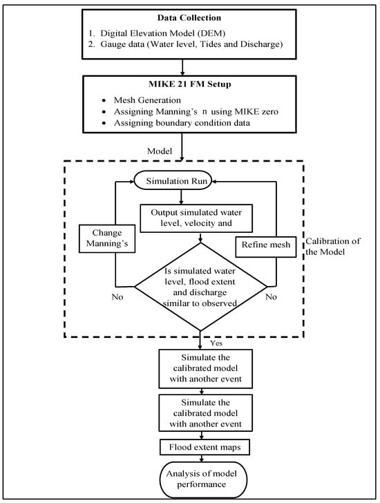
Figure 2.
Flowchart of processes involved in the MIKE 21 hydrodynamic simulation.
3.1. Data Collection
To carry out this study, we collected DEM bathymetry data, water level, flow data, tidal data, flood measurement data, and flood extent satellite data. Data collected for the study, with its resolution and sources, are shown in Table 1.

Table 1.
Data collected and sources for the study.
3.2. Hydrodynamic Model
The model used in this study was DHI MIKE-21 FM, which is a two-dimensional (2D), depth-averaged hydrodynamic model, with a numerical solution based on the incompressible Reynolds averaged Navier–Stokes equations while using the finite volume method to solve the shallow water equations [47]. In the shallow water hydrodynamic equations, due to the stability constraint of the explicit scheme, the Courant–Friedrich–Levy (CFL) condition needs to be fulfilled, which can be calculated using Equation (1). Critical CFLHD values are recommended to be set at 0.8, to fully secure the stability of the numerical scheme [48].
where h, is the local water depth; Δt is the interval of time step; Δx and Δy are typical length scales of meshes in the x and y direction, respectively, and u and v are the velocity components. The governing equation may not account for the wrong topography representation and its subsequent errors in the results. The correct discretization of mesh elements and limiting CFLHD can lead to correct results. MIKE 21 governing equations are attained by the integration of the horizontal momentum and continuity equation over depth h = ; the following shallow water 2D equations are defined in Equations (2)–(4):
where t is the time, and y are Cartesian coordinates, d is the still water depth, h is the total water depth, s is the discharge, is the reference density of water, is water density, is atmospheric pressure (Pa), are radiation stress components, which represent the momentum flux exerted by surface gravity waves on the water column, affecting the transport of water and sediments in coastal and estuarine environments. are y and x directions depth-averaged velocity, , , , are lateral stress components are surface wind stress components, g is the acceleration due to gravity, f is the Coriolis parameter, , are velocity by which water is discharged into the ambient water, are bottom stress components and is the water surface elevation.
Although Equations (2)–(4) do not explicitly include a turbulence model, turbulence is represented implicitly in the MIKE 21 hydrodynamic model through the eddy viscosity term. The Smagorinsky factor is a parameter used to estimate horizontal eddy viscosity and provides a simplified turbulence closure for depth-averaged flows. It enhances the model’s ability to simulate sub-grid scale mixing and diffusion, particularly in regions with strong velocity gradients, such as estuarine mouths or river bends.
In our study, the Smagorinsky factor was used to control the level of eddy viscosity, thereby influencing the numerical diffusion applied to the momentum equations. This contributes to model stability and ensures a physically consistent representation of flow structures, especially during high-energy events such as storm surges and compound flooding.
While a detailed turbulence model is not explicitly formulated in this context, the Smagorinsky approach is commonly adopted in large-scale hydrodynamic modelling for its computational efficiency and adequate performance in simulating flow patterns in coastal and estuarine systems
3.3. Mesh Generation and Cell Size Convergence
The DHI MIKE mesh generation tool allows the user to design the element resolution by describing the maximum element area, Amax. For the majority of mesh structure elements, approximate equilateral triangles can be attained in DHI MIKE [49] and the length of is approximately calculated using Equation (5), where 60;
In CFLHD Equation (1), as the local flow velocity is much less, it is reasonable to disregard the velocity terms, and the CFLHD can be rewritten as Equation (6). Further, the CFLHD is rearranged to Equation (7) with the reasonable assumption of.
Five meshes were generated and gradually refined until all elements fulfilled the constraint in Equation (7). Mesh quality was further enhanced by the smoothing tool to increase spatial regularity. The details of the elements, nodes, element areas CFLmax, and simulation running time in each case are given in Table 2. For the Case 1 mesh file, the Amax is 5 km2 and Amin is 70 m2, generating 95,497 elements covering the Brisbane River estuary with floodplain and the entire Moreton Bay. The mesh sizes were reduced in each subsequent case, and in Case 5, the mesh elements were 288,415. The five mesh cases with different element sizes for a small region near Brisbane City are shown in Figure 3. In these five cases, element sizes were distributed with finer elements inside the Brisbane River and coarser elements inside Moreton Bay. In all cases, the time step, Δt, was set as 30 s to fulfil the critical CFLHD of 0.8. A larger number of elements were estimated to involve a much lengthier time to complete the simulations. For the one-month simulation of the flood event in BRE and Moreton Bay, the running time was approximately 11, 13, 18, 28, and 36 h for each case, respectively.
Table 2.
Statistics of mesh resolution cases.
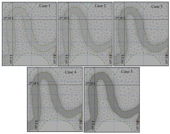
Figure 3.
Five cases of mesh resolution near Brisbane City were used in the modelling.
The computational mesh grid size was reduced in an iteration to observe the effect on simulated water levels and computational time. The mesh grid size was modified until the increase or decrease of size had a considerable effect on water levels and computational time. When there was no considerable change in the simulated water levels and computational time was increased substantially, we then stopped the mesh changing and adopted the mesh resolution with confidence, as it was the optimum size with computational time and simulated water levels.
The bathymetric data, longitudinal profile, and cross-section comparison are shown in Figure 4. By using a coarser cell size and uncontrolled data, the cross-section representation changed as compared to finer cell and controlled data (Figure 4e).
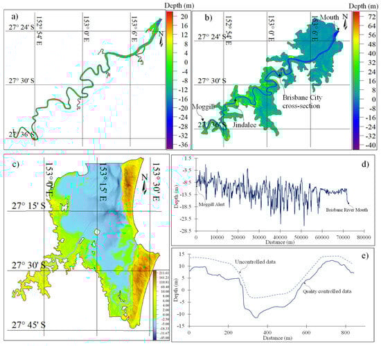
Figure 4.
Bathymetry of (a) Brisbane River; (b) Brisbane River and floodplain; (c) Brisbane River floodplains and Moreton Bay; (d) Longitudinal profile of Brisbane River; (e) Brisbane River cross-section at Brisbane city.
3.4. Future Scenarios of Storm Surge
As the sea-level rise projections range is wide enough, along the Australian coast, sea-level growth may be 10% higher [50]. A research study presented flood simulation cases for four future climate periods—2030, 2050, 2070, and 2100—in the Brisbane River Estuary (BRE), as shown in Table 3 [51]. The 100-year storm tide level used for the present-day base scenario (2.5 m) was obtained from the Queensland Department of Environment and Resource Management (DERM, 2012) storm tide study for Brisbane, a value commonly used for flood risk assessments in the region [15].
Table 3.
Proposed climate parameters for inclusion in the BRE flood risk study.
Based on these four scenarios, storm tide inputs at Brisbane Bar were used to simulate the flooding behaviour in the BRE under low flow events (Figure 5). The time series shown in Figure 5 was generated by superimposing the 100-year storm tide level (2.5 m) on the astronomical tidal signal at Brisbane Bar, using tidal constituents sourced from the Queensland Government data portal. For future scenarios, the storm tide height was adjusted according to the sea-level rise projections listed in Table 3, and then combined with the tidal series to produce synthetic future storm tide time series. Thus, Figure 5 represents the synthesized water level time series for each climate scenario, reflecting both tidal variation and projected storm tide increases under sea-level rise.
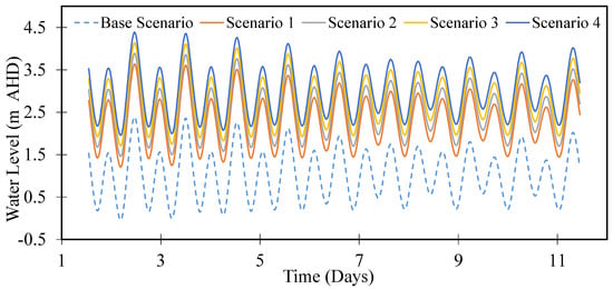
Figure 5.
Input data for various scenarios of storm surge tide at Brisbane Bar.
3.5. Model Setup
In the model, five meshes were generated, and the element sizes were adjusted using a mesh resolution test. Finally, a range from 34 m2 to 100,000 m2, with a total of 288,415 unstructured elements and 148,697 nodes, was used in the MIKE 21 domain area. The observed time-varying water level was used as the upstream boundary to the hydrodynamic model, and the tidal level observations at three stations (i.e., Amity Point, Runaway Bay Point, and Beacon M2 Point) were adopted to set the lower boundary condition of the model (Figure 4). The model was initially set up by using bathymetric data of the Brisbane River (Figure 4a) and 2006 low flow data and tidal data as boundary conditions (Figure 6a,b). Then the model was extended to floodplain areas (Figure 4b), and the years 2013 and 2011 flood and tidal data (Figure 6c,d) were used for the model performance. Finally, the model included BRE and Moreton Bay (Figure 4c) with 2011 flood and tidal data (Figure 6e–h).
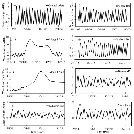
Figure 6.
(a–h) MIKE 21 model input boundary water level and tidal data.
Currently, the MIKE-21 model has not considered evaporation, precipitation, wind direction, and wind speed. The initial water surface elevation of 0.1 m was used, while the initial water flow velocities were fixed to zero across the model area. The minimum time step is limited to 0.1 s to keep the target Courant–Friedrichs–Lewy (CFL) number below 1.0. The thresholds hdry (drying depth = 0.005 m) < hflood (flooding depth = 0.05 m) < hwet (wetting depth = 0.1 m) were used to describe the change of wetting and drying in the model [40]. In a hydrodynamic model, bed resistance is an important factor that controls river flow behaviour. While calibrating the model, Manning’s n is changed within an acceptable limit to bridge the gap between observed and simulated water levels. Manning’s M (reciprocal to Manning’s n) is used in the model to specify the bed resistance. In the present study, the Manning number for the Brisbane River floodplains and Moreton Bay is used as (M = 10–38 m1/3/s) which was based on literature values from previous modelling calibration of Brisbane River [1,34] and Moreton Bay [36]. The Smagorinsky factor of eddy viscosity (Cs = 0.28) based on the literature review [40,52] was adopted to perform the hydrodynamic simulation and model validation. Model calibration and validation are described in detail in Section 4.
3.6. Model Performance Evaluation Indices
To compare the observed and simulated results, various statistical methods were used e.g., Nash–Sutcliffe model efficiency coefficient (Ens), Root Mean Square Error (RMSE), and Coefficient of determination (R2). Nash–Sutcliffe coefficient (Ens) was used to assess the MIKE 21 model predictive power and to describe quantitatively the accuracy of simulation results with the observed values. It is defined in Equation (8):
where Xmodel is simulated values at the time i and Xobs are observed values. Primarily, model efficiency close to 1, represents accurate results. The root mean square error (RMSE) was used to measure the difference between simulated values by a model and the observed values, it is defined in Equation (9):
where, Xmodel is simulated values at the time i, Xobs is observed values.
4. Results and Discussion
4.1. Calibration and Validation of the Model
A comparison between simulated and observed water levels at Brisbane City gauge for the low flow event confined inside the Brisbane River during the year 2006 is shown in Figure 7a. For the year 2013 high flow event, spreading over floodplains, the comparison between observed and simulated water levels at the Brisbane City gauge is shown in Figure 7b. The hydrodynamic model is calibrated against the low flow events in 2006 and 2013, and to increase the predictive power, it is validated for the high flow event of 2011. For the 2011 flood event, extending over floodplains, the simulated results are compared with those observed at Brisbane City and Brisbane Bar gauge, as shown in Figure 7c,d. The performance indices for calibrating gauging stations are shown in Table 4. The statistical results showed that Ens of water levels varied from 0.84 to 0.95, RMSE values were less than 0.3 and R2 values varied from 0.85 to 0.96, which shows a good match between the observed and simulated water levels.
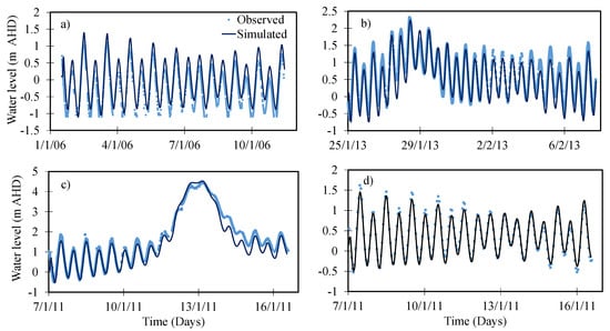
Figure 7.
Observed and simulated water levels at (a) Brisbane City for the year 2006; (b) Brisbane City for the year 2013; (c) Brisbane City for the year 2011; and (d) Brisbane Bar for the year 2011.
Table 4.
Performance indices for the calibration and validation of gauging stations of 2006, 2013, and 2011 flow events.
The result of the comparison between observed and simulated flood extent is shown in Figure 8. Brisbane City experienced a major flood from 12 January at 10:00 am to 13 January at 6:00 pm of 32 h duration [16]. The observed flood extent on 13 January 2011 at 04:00 am compared well with the simulated flood extent. The model predictions of flood extent area are 90% accurate while using Mesh Case 5, which is substantially improved as compared to [1] with 66.9% accuracy. The model correctly regenerated most of the Oxley Creek floodplain and the largest areas of observed flooding below the Jindalee floodplain (Figure 8), due to the correct representation of bathymetry and boundary data, which leads to correct flood extent assessment as discussed by [44]. However, the model underestimated the flood extent in very small tributaries adjoining the Brisbane River, due to the lack of a finer mesh size in these areas, which would lead to an increase in computational time. Based on the model’s good representation of most of the floodplain areas, the results can be used for future predictions.
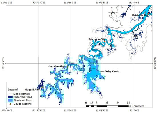
Figure 8.
Simulated and observed inundation area of Brisbane catchment for the 2011 flood event.
4.2. Mesh Resolution Effects on Discharge
The model performance results for the simulated discharge by using different mesh resolutions at the Brisbane City gauge are shown in Figure 9. The results display a higher difference of coarser mesh with the observed data, and as mesh size becomes finer, the observed and simulated discharges reduce, indicating that the simulated discharges were correctly represented by the finer mesh resolution, as also proposed by [53]. The percentage difference in the peak value of simulated discharges with the estimated discharge by Barton, Syme [36] was 16.54%, 14%, 12.19%, 2.88%, and 2.7% from Case 1 to Case 5, respectively. The decreasing difference with observed values showed that the quality of simulation results was gradually enhanced by refining the mesh size; conversely, further decreases in mesh size create comparatively less difference from Cases 4 to 5. Further, it was found that with a coarser mesh size, the hydrodynamic features (i.e., current velocity and discharge) of the BRE might not be reproduced in the simulation; however, with a finer mesh size, the performance of the model was enhanced, which agreed with the findings of other studies [44].
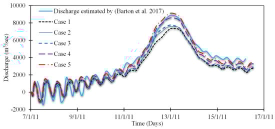
Figure 9.
Comparison of simulated discharge at Brisbane City gauge with estimated discharge by [36] for various mesh resolution cases.
4.3. Modelled Water Levels and Flood Extents Under Varying Boundaries
The results of the interaction of storm-tide and fluvial flooding mechanisms via modelling a compound flooding event in the BRE are shown in Figure 10. The simulated and observed water levels with and without river and tidal boundaries are presented at three-gauge locations in Figure 10. The flood extents corresponding to these boundaries are presented in Figure 11. Comparison of results at the Jindalee gauge station (Figure 10a) with and without tidal boundaries shows that the peak water level varied slightly, with a 0.62 m reduction at peak level without tidal input. Further, without a tidal boundary, the hydrograph has attained smooth rising and falling limbs without showing any tidal variations. On the other hand, without a discharge boundary, i.e., Q = 0, the tidal input moved up to the Jindalee gauge and caused a slight reduction in tidal levels. The comparison of peak water level with and without a tidal boundary at Brisbane City gauge (Figure 10b) shows that the difference in peak flood level could be as high as 0.12 m, while without a riverine boundary, the water level followed the tidal wave pattern at Brisbane City gauge. At Brisbane Bar, without a tidal boundary, the water level followed a straight line, with a slight increase in water level during the flood days, while the tidal level at Brisbane Bar was slightly reduced without a riverine boundary (Figure 10c).
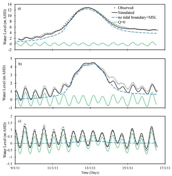
Figure 10.
Modelled and observed water levels for different boundaries (i.e., without tidal boundary = mean sea level (MSL); without discharge boundary, i.e., Q = 0) at three gauges; (a) Jindalee; (b) Brisbane City and; (c) Brisbane Bar.
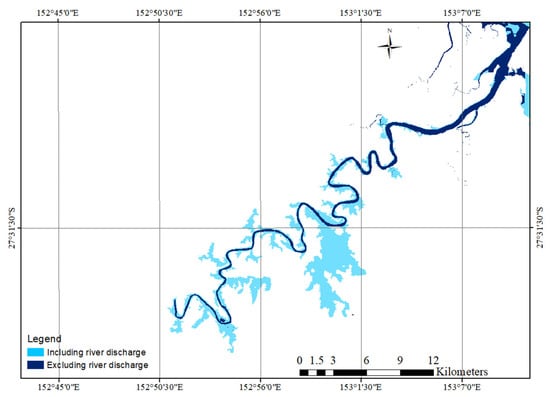
Figure 11.
Simulated maximum flood extents at the Brisbane catchment for the 2011 flood with and without river discharge using the two open boundary model setups.
Modelled flood extents show a great difference between the two modelling set-ups. The spatial differences in flood extent resulting from simulations with and without river discharge are shown in Figure 11. The flood extent resulting from the combination of river discharge and tidal water levels is shown as lighter blue areas in Figure 11, whereas dark blue areas show the flood extent resulting only from tidal water inputs. The comparison of simulated flood extents resulting from these simulations shows variation in the lower BRE floodplain. The inclusion of river discharge caused substantial flood extent within the Oxley Creek floodplain, while without river discharge, the tidal water level was confined within the BRE and caused flood extent in floodplain areas.
4.4. Modelled Flood Extents Under Future Storm Surge Cases
Simulated results of flood extent in BRE under the four storm surge scenarios (Figure 4) are presented in Figure 12. The baseline simulation, representing normal tidal conditions, indicated no significant flooding within the BRE. This suggests that under normal conditions, the tidal regime is contained within the estuary’s boundaries.
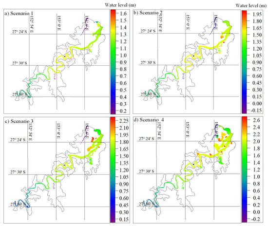
Figure 12.
Simulated flood extents of the Brisbane catchment in four scenarios of storm surge; (a) year 2030; (b) year 2050; (c) year 2070; (d) year 2100.
However, the future storm surge scenarios revealed a progressive increase in flood extent with rising tidal levels. Scenario 1, projecting a 25% increase in tidal level, resulted in only very minor flooding, localized primarily near the estuary mouth (Figure 12a). The limited impact observed in Scenario 1 suggests that the BRE has some capacity to absorb a moderate increase in tidal forcing, with the tidal level remaining just below the minor flood level of 1.7 m.
As the tidal level increased to 50% in Scenario 2, the simulations showed a more pronounced impact, with the tidal level exceeding the minor flood level and causing inundation in the tributaries adjoining the BRE (Figure 12b). This indicates a critical threshold being crossed, where the increased tidal forcing begins to overcome the estuary’s natural containment capacity, leading to more widespread flooding.
Scenarios 3 and 4, representing more extreme increases in tidal levels, demonstrated a substantial expansion of the flood extent, particularly near the BRE mouth and the Brisbane City gauge area (Figure 12c,d). In these scenarios, the flood water level surpassed the minor flood level and reached the medium flood level of 2.6 m, highlighting the potential for significant inundation under severe storm surge conditions.
4.5. Discussion of Flood Extent Progression
The progression of flood extent across the four scenarios reveals a clear correlation between increasing tidal levels and the spatial extent of inundation. The transition from negligible flooding in Scenario 1 to widespread inundation in Scenarios 3 and 4 underscores the sensitivity of the BRE to relatively small changes in sea level.
The localized flooding near the estuary mouth in the initial scenarios suggests that this region is the most vulnerable to increased tidal forcing. As the tidal level rises, the inundation expands inland, affecting low-lying tributaries and, in the most extreme scenarios, threatening the Brisbane City gauge area. This inland progression of flooding is consistent with the understanding of tidal dynamics, where increased sea levels push further upstream, impacting areas that are normally beyond the reach of tidal influence.
Further analysis incorporating the 2011 and 2013 flood events in combination with the Extreme Storm Surge Scenario 4 (Figure 13) revealed the potential for compound flooding, where the joint probability of riverine flow and storm surge significantly exacerbates the flood extent [51]. The simulation results indicate that the floodwater level during the 2011 flood at the Brisbane city gauge, which was observed as 4.46 m, could increase to 5 m under future storm surge conditions combined with increased rainfall. This increase in floodwater level leads to a greater flood extent and depth in the floodplain area, with more severe flooding at the BRE mouth. Similarly, the flood height for the 2013 flood increased from 2.24 m to 3.01 m due to the combined effect of river and storm surge, exceeding the medium flood level of 2.6 m at the Brisbane city gauge and resulting in flooding in the Oxley Creek area.
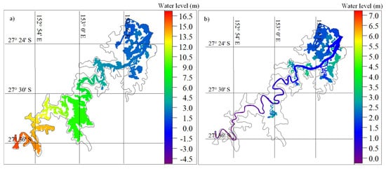
Figure 13.
Simulated flood extents of Brisbane catchment; (a) 2011; and (b) 2013 flood events in combination with Future Storm Surge Scenario 4.
The modelling results emphasize the importance of considering the combined effects of riverine flow and storm surge in flood inundation studies and coastal planning within the BRE. The interaction between these two factors can lead to non-linear increases in flood extent and depth, posing a significant challenge for flood risk management. The results also highlight how increasing tidal height can impede low river flow, pushing tidal influence further into the BRE and causing both minor and moderate flooding.
5. Conclusions
To simulate flood height and extent in the Brisbane River Estuary, mesh resolutions and combined flood effects were analysed using the MIKE 21 Model. The MIKE 21 hydrodynamic model was calibrated and validated for the years 2006, 2013, and 2011 flow events, with a flow Nash–Sutcliffe coefficient (Ens) between 0.84 and 0.95 at all gauges. The model simulated the flooding extent of BRE, showing more than 90% accuracy. This confirmed that the MIKE 21 model can dynamically simulate and replicate the flows with a compound flood event and can be used for planning the coastal estuaries for future compound flood events.
Compound flood event simulation results emphasized that not considering the interaction of various flooding drivers has caused a 0.62 m and 0.12 m reduction in flood levels at the Jindalee and Brisbane City gauges, while leading to a substantial underestimation of flood extent. Results endorse the consideration of tidal and riverine flooding drivers mutually for coastal flood extent assessments in estuaries.
Simulated results of flood extent in BRE based on four storm surge scenarios show that the flooding level would cross the medium flood level at the Brisbane City gauge. Further, with the 2011 and 2013 floods with Storm Surge Scenario 4, it was demonstrated that the flood level will increase by 12% and 34%, respectively, and the flood extent will increase in Oxley Creek and near the BRE mouth.
Modelling shows that mesh resolution is an important aspect of the appropriate evaluation of the flood extent in coastal estuaries.
The results show that a flood hydrodynamics study of BRE by using mesh resolution with joint probability compound flood events and considering future storm surge analysis would be helpful for coastal managers in the planning and management of coastal projects.
The findings are significant for the understanding of how the incorporation of the joint events is necessary to better model flooding processes in river estuaries or coastal catchments that can be affected by both the tidal inflow and the river discharges.
To simulate flood height and extent in the Brisbane River Estuary (BRE), mesh resolutions and combined flood effects were analysed using the MIKE 21 Model. The MIKE 21 hydrodynamic model was calibrated and validated for the years 2006, 2013, and 2011 flow events, with a flow Nash–Sutcliffe coefficient (Ens) between 0.84 and 0.95 at all gauges. The model simulated the flooding extent of BRE with more than 90% accuracy. This confirmed that the MIKE 21 model can dynamically simulate and replicate the flows associated with compound flood events and can be used for planning coastal estuaries under future compound flood scenarios.
Compound flood simulation results emphasized that neglecting the interaction of various flooding drivers can lead to an underestimation of flood levels—by 0.62 m and 0.12 m at Jindalee and Brisbane City gauges, respectively—and a significant underestimation of the flood extent. These results underscore the importance of considering both tidal and riverine flooding drivers in flood extent assessments for estuarine regions.
Simulated results of flood extent in BRE, based on four storm surge scenarios, indicate that flood levels would exceed the medium flood level at the Brisbane City gauge. Additionally, under Scenario 4 combined with the 2011 and 2013 historical floods, the flood level is projected to increase by 12% and 34%, respectively, with expanded flood extent in Oxley Creek and near the BRE mouth.
The modelling also shows that mesh resolution is a critical factor for the accurate evaluation of flood extents in coastal estuaries. Overall, this study demonstrates that simulating flood hydrodynamics using mesh resolution, joint probability compound flood events, and future storm surge analysis can provide valuable insights for coastal managers planning flood mitigation and climate resilience strategies.
While the current study provides important insights into compound flooding in the Brisbane River Estuary, it has some limitations. Most notably, the modelling framework does not explicitly incorporate hydraulic structures such as bridges, culverts, or floodgates along the river, nor does it simulate reservoir operations that can significantly affect flood propagation. Prior studies have shown the importance of including such features for more realistic flood modelling. Future work should aim to integrate these hydraulic structures and reservoir operations into the model to further improve the accuracy of flood extent predictions and risk assessments in the BRE and similar coastal systems.
Author Contributions
U.K.: Conceptualization, methodology, writing—original draft, review editing, and investigation. M.S. (Mariam Sajid): Investigation, writing, review and editing. M.Z.B.R.: Review and editing. U.I. Review and editing: E.J. Review and editing. S.-Q.Y.: Conceptualization, review, editing, and supervision. M.S. (Muttucumaru Sivakumar): Review editing and supervision. All authors have read and agreed to the published version of the manuscript.
Funding
This research received no external funding.
Data Availability Statement
Data is contained within the article.
Acknowledgments
The authors would like to thank the Queensland Government Departments for providing all necessary input data. Special thanks to Daryl Metters (Department of Environment and Science), Jim Fear (SEQ Water), Paul Boswood (Department of Environment and Science), Paul Birch (Bureau of Meteorology) and Paul Finger (Maritime Safety Queensland). We are thankful to DHI for providing the MIKE 21 license. The authors would also like to thank Caroline Lai and Méven Robin Huiban for providing technical support for MIKE 21.
Conflicts of Interest
The authors declare no conflict of interest.
References
- Liu, X.; Lim, S. Flood Inundation Modelling for Mid-Lower Brisbane Estuary. River Res. Appl. 2017, 33, 415–426. [Google Scholar] [CrossRef]
- Khalil, U.; Khan, N.M. Floodplain Mapping for Indus River: Chashma–Taunsa Reach. Pak. J. Eng. Appl. Sci. 2017, 20, 30–48. [Google Scholar]
- Geravand, F.; Hosseini, S.M.; Ataie-Ashtiani, B. Influence of river cross-section data resolution on flood inundation modeling: Case study of Kashkan river basin in western Iran. J. Hydrol. 2020, 584, 124743. [Google Scholar] [CrossRef]
- Sadler, J.M.; Goodall, J.L.; Behl, M.; Bowes, B.D.; Morsy, M.M. Exploring real-time control of stormwater systems for mitigating flood risk due to sea level rise. J. Hydrol. 2020, 583, 124571. [Google Scholar] [CrossRef]
- Vitousek, S.; Barnard, P.L.; Fletcher, C.H.; Frazer, N.; Erikson, L.; Storlazzi, C.D. Doubling of coastal flooding frequency within decades due to sea-level rise. Sci. Rep. 2017, 7, 1399. [Google Scholar] [CrossRef]
- Pachauri, R.K.; Allen, M.R.; Barros, V.R.; Broome, J.; Cramer, W.; Christ, R.; Church, J.A.; Clarke, L.; Dahe, Q.; Dasgupta, P.; et al. Climate Change 2014: Synthesis Report. Contribution of Working Groups I, II and III to the Fifth Assessment Report of the Intergovernmental Panel on Climate Change; IPCC: Geneva, Switzerland, 2014.
- Van Coppenolle, R.; Temmerman, S. A global exploration of tidal wetland creation for nature-based flood risk mitigation in coastal cities. Estuarine. Coast. Shelf Sci. 2019, 226, 106262. [Google Scholar] [CrossRef]
- Hallegatte, S.; Green, C.; Nicholls, R.J.; Corfee-Morlot, J. Future flood losses in major coastal cities. Nat. Clim. Change 2013, 3, 802. [Google Scholar] [CrossRef]
- Tsoukala, V.K.; Chondros, M.; Kapelonis, Z.G.; Martzikos, N.; Lykou, A.; Belibassakis, K.; Makropoulos, C. An integrated wave modelling framework for extreme and rare events for climate change in coastal areas–the case of Rethymno, Crete. Oceanologia 2016, 58, 71–89. [Google Scholar] [CrossRef]
- McCallum, I.; Liu, W.; See, L.; Mechler, R.; Keating, A.; Hochrainer-Stigler, S.; Mochizuki, J.; Fritz, S.; Dugar, S.; Arestegui, M.; et al. Technologies to support community flood disaster risk reduction. Int. J. Disaster Risk Sci. 2016, 7, 198–204. [Google Scholar] [CrossRef]
- Sulis, A.; Frongia, S.; Liberatore, S.; Zucca, R.; Sechi, G.M. Combining water supply and flood control purposes in the Coghinas Basin (Sardinia, Italy). Int. J. River Basin Manag. 2018, 18, 13–22. [Google Scholar] [CrossRef]
- UNISDR. Global Assessment Report on Disaster Risk Reduction 2015: Making Development Sustainable: The Future of Disaster Risk Management; United Nations International Strategy for Disaster Reduction: Geneva, Switzerland, 2015. [Google Scholar]
- Lee, E.H.; Kim, J.H. Development of a flood-damage-based flood forecasting technique. J. Hydrol. 2018, 563, 181–194. [Google Scholar] [CrossRef]
- Syme, B. Executive Summary and Recommendations Brisbane River Strategic Floodplain Management Plan; BMT WBM: Brisbane, Australia, 2019. [Google Scholar]
- Barton, C.; Wallace, S.; Syme, B.; Wong, W.T.; Onta, P. Brisbane River catchment flood study: Comprehensive hydraulic assessment overview. In Proceedings of the Floodplain Management Association National Conference, Brisbane, Australia, 19–22 May 2015. [Google Scholar]
- van den Honert, R.C.; McAneney, J. The 2011 Brisbane floods: Causes, impacts and implications. Water 2011, 3, 1149–1173. [Google Scholar] [CrossRef]
- Rice, M.; Karoly, D.; Arndt, D.; Comer, J.; O’Rourke, S. Eye of the Storm: How Climate Pollution Fuels More Intense and Destructive Cyclones; Climate Council: London, UK, 20 March 2025. [Google Scholar]
- Neumann, J.E.; Price, J.; Chinowsky, P.; Wright, L.; Ludwig, L.; Streeter, R.; Jones, R.; Smith, J.B.; Perkins, W.; Jantarasami, L.; et al. Climate change risks to US infrastructure: Impacts on roads, bridges, coastal development, and urban drainage. Clim. Change 2014, 131, 97–109. [Google Scholar] [CrossRef]
- Karim, M.F.; Mimura, N. Impacts of climate change and sea-level rise on cyclonic storm surge floods in Bangladesh. Glob. Environ. Change 2008, 18, 490–500. [Google Scholar] [CrossRef]
- Zheng, F.; Westra, S.; Leonard, M.; Sisson, S.A. Modeling dependence between extreme rainfall and storm surge to estimate coastal flooding risk. Water Resour. Res. 2014, 50, 2050–2071. [Google Scholar] [CrossRef]
- Leonard, M.; Westra, S.; Phatak, A.; Lambert, M.; van den Hurk, B.; McInnes, K.; Risbey, J.; Schuster, S.; Jakob, D.; Stafford-Smith, M. A compound event framework for understanding extreme impacts. Wiley Interdiscip. Rev. Clim. Change 2014, 5, 113–128. [Google Scholar] [CrossRef]
- Wu, W.; Westra, S.; Leonard, M. Estimating the Probability of Compound Floods in Estuarine Regions. Hydrol. Earth Syst. Sci. Discuss. 2020, 25, 2821–2841. [Google Scholar] [CrossRef]
- Green, J.; Haigh, I.; Quinn, N.; Neal, J.; Wahl, T.; Wood, M.; Eilander, D.; de Ruiter, M.; Ward, P.; Camus, P. A comprehensive review of compound flooding literature with a focus on coastal and estuarine regions. EGUsphere 2024, 2024, 1–108. [Google Scholar] [CrossRef]
- Treloar, P.; Taylor, D.; Prenzler, P. Investigation of wave induced storm surge within a large coastal embayment-Moreton Bay (Australia). Coast. Eng. Proc. 2011, 1, 22. [Google Scholar] [CrossRef]
- Torres, J.M.; Bass, B.; Irza, N.; Fang, Z.; Proft, J.; Dawson, C.; Kiani, M.; Bedient, P. Characterizing the hydraulic interactions of hurricane storm surge and rainfall–runoff for the Houston–Galveston region. Coast. Eng. 2015, 106, 7–19. [Google Scholar] [CrossRef]
- Svensson, C.; Jones, D.A. Dependence between sea surge, river flow and precipitation in south and west Britain. Hydrol. Earth Syst. Sci. 2004, 8, 973–992. [Google Scholar] [CrossRef]
- Hawkes, P.; Svensson, C. Joint Probability: Dependence Mapping and Best Practice; T02-06-16; Defra/Environment Agency: London, UK, 2006.
- Zheng, F.; Westra, S.; Sisson, S.A. Quantifying the dependence between extreme rainfall and storm surge in the coastal zone. J. Hydrol. 2013, 505, 172–187. [Google Scholar] [CrossRef]
- Chen, A.S.; Evans, B.; Djordjević, S.; Savić, D.A. Multi-layered coarse grid modelling in 2D urban flood simulations. J. Hydrol. 2012, 470–471, 1–11. [Google Scholar] [CrossRef]
- Son, A.-L.; Kim, B.; Han, K.-Y. A Simple and Robust Method for Simultaneous Consideration of Overland and Underground Space in Urban Flood Modeling. Water 2016, 8, 494. [Google Scholar] [CrossRef]
- Bevacqua, E.; Vousdoukas, M.I.; Zappa, G.; Hodges, K.; Shepherd, T.G.; Maraun, D.; Mentaschi, L.; Feyen, L. More meteorological events that drive compound coastal flooding are projected under climate change. Commun. Earth Environ. 2020, 1, 47. [Google Scholar] [CrossRef]
- Kumbier, K.; Carvalho, R.C.; Vafeidis, A.T.; Woodroffe, C.D. Investigating compound flooding in an estuary using hydrodynamic modelling: A case study from the Shoalhaven River, Australia. Nat. Hazards Earth Syst. Sci. 2018, 18, 463–477. [Google Scholar] [CrossRef]
- Queensland Floods Commission Inquiry Report, Q. Queensland Floods Commission of Inquiry; Complete list of Final Report Recommendations; Royal Commissions: Brisbane, Australia, 2011.
- Yu, Y. Numerical Study of Hydrodynamic and Sediment Transport Within the Brisbane River Estuary and Moreton Bay, Australia. Ph.D. Thesis, Griffith University, Brisbane, Australia, 2017. [Google Scholar]
- Mani, P.; Chatterjee, C.; Kumar, R.J.N.H. Flood hazard assessment with multiparameter approach derived from coupled 1D and 2D hydrodynamic flow model. Nat. Hazards 2014, 70, 1553–1574. [Google Scholar]
- Barton, C.; Syme, B.; Ryan, P.; Rodgers, B.; Jensen, R. Milestone Report 2: Fast Model Development and Calibration Comprehensive Hydraulic Assessment; BMT WBM: Brisbane, Australia, 2017. [Google Scholar]
- Pellikka, H.; Leijala, U.; Johansson, M.M.; Leinonen, K.; Kahma, K.K. Future probabilities of coastal floods in Finland. Cont. Shelf Res. 2018, 157, 32–42. [Google Scholar] [CrossRef]
- Liu, Y.; Yang, S.Q.; Jiang, C.; Sivakumar, M.; Enever, K.; Long, Y.; Deng, B.; Khalil, U.; Yin, L. Flood Mitigation Using an Innovative Flood Control Scheme in a Large Lake: Dongting Lake, China. Appl. Sci. 2019, 9, 2465. [Google Scholar] [CrossRef]
- Li, Y.; Yao, J. Estimation of transport trajectory and residence time in large river–lake systems: Application to Poyang Lake (China) using a combined model approach. Water 2015, 7, 5203–5223. [Google Scholar] [CrossRef]
- Li, Y.; Zhang, Q.; Tan, Z.; Yao, J. On the hydrodynamic behavior of floodplain vegetation in a flood-pulse-influenced river-lake system (Poyang Lake, China). J. Hydrol. 2020, 585, 124852. [Google Scholar] [CrossRef]
- Khalil, U.; Yang, S.Q.; Sivakumar, M.; Enever, K.; Sajid, M.; Bin Riaz, M.Z. Investigating an Innovative Sea-Based Strategy to Mitigate Coastal City Flood Disasters and Its Feasibility Study for Brisbane, Australia. Water 2020, 12, 2744. [Google Scholar] [CrossRef]
- Haldar, R.; Khosa, R.; Gosain, A. Impact of Anthropogenic Interventions on the Vembanad Lake System. In Water Resources and Environmental Engineering I; Springer: Berlin/Heidelberg, Germany, 2019; pp. 9–29. [Google Scholar]
- Liu, J.; Sivakumar, M.; Yang, S.; Jones, B. Salinity Modelling and Management of the Lower Lakes of the Murray–Darling Basin, Australia. In Water Pollution XIV; University of Wollongong: Wollongong, Australia, 2018; pp. 257–268. [Google Scholar]
- Shrestha, A.; Bhattacharjee, L.; Baral, S.; Thakur, B.; Joshi, N.; Kalra, A.; Gupta, R. Understanding Suitability of MIKE 21 and HEC-RAS for 2D Floodplain Modeling; American Society of Civil Engineers: Reston, VA, USA, 2020; pp. 237–253. [Google Scholar]
- Eyre, B.; Hossain, S.; McKee, L. A suspended sediment budget for the modified subtropical Brisbane River estuary, Australia. Estuar. Coast. Shelf Sci. 1998, 47, 513–522. [Google Scholar] [CrossRef]
- Wolanski, E. Estuaries of Australia in 2050 and Beyond; Springer: Berlin/Heidelberg, Germany, 2014. [Google Scholar]
- DHI. MIKE 21 & MIKE 3 Flow Model FM, Hydrodynamic and Transport Module Scientific Documentation; DHI Group: Hørsholm, Denmark, 2017. [Google Scholar]
- DHI. MIKE 21 Hydrodynamic Module Step-by-Step Training Guide; DHI Group: Hørsholm, Denmark, 2014. [Google Scholar]
- DHI. MIKE ZERO, Mesh Generator, Step-by-Step Training Guide; DHI Group: Hørsholm, Denmark, 2012. [Google Scholar]
- IPCC. Fourth Assessment Report of the IPCC; IPCC: Geneva, Switzerland, 2007.
- Ayre, R. Brisbane River Catchment Flood Study: Comprehensive Hydrologic Assessment; Aurecon Australasia: Brisbane, Australia, 2017. [Google Scholar]
- DHI. MIKE 21 Flow Model FM, Hydrodynamic Module, User Guide; DHI Group: Hørsholm, Denmark, 2017. [Google Scholar]
- Teng, J.; Jakeman, A.; Vaze, J.; Croke, B.; Dutta, D.; Kim, S. Flood inundation modelling: A review of methods, recent advances and uncertainty analysis. Environ. Model. Softw. 2017, 90, 201–216. [Google Scholar] [CrossRef]
Disclaimer/Publisher’s Note: The statements, opinions and data contained in all publications are solely those of the individual author(s) and contributor(s) and not of MDPI and/or the editor(s). MDPI and/or the editor(s) disclaim responsibility for any injury to people or property resulting from any ideas, methods, instructions or products referred to in the content. |
© 2025 by the authors. Licensee MDPI, Basel, Switzerland. This article is an open access article distributed under the terms and conditions of the Creative Commons Attribution (CC BY) license (https://creativecommons.org/licenses/by/4.0/).