Article

A Numerical Study on the Effect of the Coriolis Force on the Sediment Exchange Between the Yangtze River Estuary and Hangzhou Bay

by
Jia Tang
1,
Peng Hu
1,2,*,
Zixiong Zhao
1,
Junyu Tao
1,
Aofei Ji
1,
Zihao Feng
1 and
Linwei Dai
2
1
State Key Laboratory of Ocean Sensing & Ocean College, Zhejiang University, Zhoushan 316021, China
2
Ocean Research Center of Zhoushan, Zhejiang University, Zhoushan 316021, China
*
Author to whom correspondence should be addressed.
Water 2025, 17(7), 1011; https://doi.org/10.3390/w17071011
Submission received: 23 February 2025 / Revised: 25 March 2025 / Accepted: 27 March 2025 / Published: 29 March 2025
(This article belongs to the Special Issue Coastal Management and Nearshore Hydrodynamics, 2nd Edition)

Abstract

:
A GPU-accelerated shallow water model with a local time-step (LTS) is employed in this work to examine how the Coriolis forces affect the tidal level difference and, consequently, the water–sediment exchange between Hangzhou Bay (HZB) and the Yangtze River Estuary. The model is applied to both idealized and realistic estuary configurations to analyze tidal level gradients between the two neighboring estuaries under different flow conditions and with and without the Coriolis force condition. The model’s accuracy in predicting tidal levels and currents was validated against field data. It is shown that the tidal level gradient is negative during flood tide, indicating a mass transfer trend from south to north, whereas the tidal level gradient is positive during ebb tide, indicating a north-to-south mass transfer. Considering sediment originates mainly from the riverine side, the sediment mass transfer may occur mainly during ebb tide, and the direction is from the Yangtze River to the HZB. This finding provides numerical evidence for previous recognition that sediment in HZB mainly comes from the Yangtze River Estuary. A comparison of the idealized and realistic estuary configurations further indicates that the contrasting bed topography enhances tidal level gradients. The findings show that by causing tidal phase changes and asymmetric tidal range modifications, the Coriolis force increases lateral water level gradients (up to 0.7 m) between the Yangtze Estuary and Hangzhou Bay. Idealized modeling further demonstrates that higher Coriolis coefficients promote sediment exchange and exacerbate water level fluctuations across estuaries. Without the Coriolis effect, the tide level distribution in adjacent estuaries is symmetrical. In the Northern and Southern Hemispheres, the tide level distribution in adjacent estuaries is the opposite. In addition, this study has shown that changes in river flow have a limited effect on water levels at stations farther from the estuary’s flow intake and therefore have a negligible effect on the water level gradient in adjacent estuaries farther away. However, topography differences have a significant effect on water level gradients in neighboring estuaries. These studies emphasize the significance of the Coriolis force in regulating sediment transport pathways in estuaries.

1. Introduction

Hangzhou Bay is characterized by significant tidal fluctuations, rapid hydrodynamic forces, and elevated sediment concentrations, typifying it as a prominent trumpet-shaped estuary with robust tidal dynamics. Hangzhou Bay’s north shore is located at the southern edge of the Yangtze River delta (see Figure 1). The two locations also frequently exchange sediment. The primary source of sediment between Hangzhou Bay and the Qiantang River estuary is the southward transport of suspended sediment from the Yangtze River into the sea, along with re-suspended sediment from the muddy regions of the Yangtze River delta [1]. In Hangzhou Bay and offshore areas, approximately 40% of the sediment transported to the sea by the Yangtze River is deposited. However, human activities have significantly altered the conditions of water and sediment. As a result of measures such as soil and water conservation and the construction of reservoirs, the volume of sediment flowing into the sea at the mouth of the Yangtze River has dramatically decreased, from 500 million tons to less than 100 million tons [2,3,4]. The reduction of sediment entering the sea at the mouth of the Yangtze River and on the north coast of Hangzhou Bay, the area where the Yangtze River connects to the sea, would unavoidably be directly influenced by significant fluctuations in both the volume of runoff and the sand content of the river [5,6]. The hydrodynamic properties of both estuaries will be affected by the reduction in sediment volume from the Yangtze River estuary into the northern shore of Hangzhou Bay. Dai et al. [5] have documented the long-term effects of sediment reduction on estuarine geomorphology. They suggest that the reduction in sediment supply can lead to changes in the equilibrium state of estuarine systems, which may manifest over longer time scales. Therefore, under the altered water–sediment conditions, it is essential to explore the main pathways and factors influencing material exchange between the two estuaries.
The dynamics of estuarine sediment transport in the Yangtze River estuary and Hangzhou Bay (HZB) are governed by complex factors such as tidal asymmetry, topographic constraints, river discharge, and the Coriolis forces. Tidal asymmetry, an important factor for waterborne substance transport, which refers to differences in the intensity and duration of flood and ebb tides, plays a crucial role in determining the direction of net sediment transport [7]. The Yangtze River estuary and Hangzhou Bay exhibit different tidal asymmetry patterns. The Yangtze River estuary is characterized by ebb-dominant tidal conditions. Field observations and previous studies have shown that the ebb tidal current speed exceeds the flood tidal current speed and that the duration of the ebb tide is longer than the duration of the flood tide [8]. In contrast, the tidal asymmetry pattern in Hangzhou Bay is more complicated. By analyzing the tidal data from several stations, it is found that the flood tide duration is shorter than the ebb tide duration at most of the stations in Hangzhou Bay, except for the Zhenhai station, where the average flood tide duration is slightly longer than the ebb tide duration [9]. This tidal asymmetry gradient between neighboring estuaries creates an inherent potential for sediment transport, as tidally dominated systems typically export sediments seaward, while flood-dominated areas enhance landward sediment transport.
Recent studies have emphasized the significant role of tidal asymmetry in shaping sediment dynamics within estuarine systems. For instance, Suh et al. [10] demonstrated that multiple coastal constructions along the west coast of South Korea altered the tidal asymmetry, shifting the system from ebb to flood dominance and significantly impacting sediment transport patterns, including increased landward sediment transport in flood-dominant systems. Similarly, Suh [11] studied the effects of sea level rise on tidal asymmetry and energy dissipation in a macro tidal bay, showing that sea level rise causes a reduction in the tidal flat area, leading to increased tidal deformation. Small changes in tidal asymmetry can significantly affect long-term sediment deposition and erosion processes. Ji et al. [12] explored the mechanisms behind tidal current asymmetry in response to land reclamations in Lingding Bay, revealing that the shoreline change shifted the flow velocity asymmetry from ebb to flood dominance, thereby impacting sediment transport pathways. Furthermore, Feng and Feng [13] investigated the role of anthropogenic activities and sea level rise in the tidal deformation of the Yellow Sea shelf, emphasizing that tidal asymmetry is highly sensitive to changes in coastal morphology and can significantly affect sediment transport and deposition.
Numerous studies have examined the primary routes and methods of sediment movement from the Yangtze River to Hangzhou Bay and Qiantang River, as well as the evident material exchange between the Yangtze River estuary and Hangzhou Bay–Qiantang River. The longitudinal transport of tidal flat sediment from the Yangtze River mouth to Hangzhou Bay is primarily caused by the water surface drop and phase difference between the southern and northern parts of Nanhui tidal flats, according to Li [14], who made this observation based on a substantial amount of measured data. The Yangtze River’s silt reaches Hangzhou Bay close to the mouth of Nanhui, and through a series of deposition and re-suspension processes, it is progressively carried to the Zhoushan coastal waters, creating the fundamental pattern of sediment entering from the north and leaving from the south.
Cao and Yan [15] separated the sediment exchange between the Yangtze River mouth and Hangzhou Bay into direct and indirect processes based on a number of factors, including the development of the Nanhui Mouth (the confluence of the Yangtze River mouth and Hangzhou Bay), the distribution of the substrate in Hangzhou Bay and the source of the material, the spatial and temporal characteristics of the distribution of the suspended sediments in Hangzhou Bay–Zhoushan coastal waters, the correlation of the salinity fields of the Yangtze River mouth and Hangzhou Bay, the mechanism of the East China Sea tidal wave rise and fall, and other factors. Chen et al. [1] examined the interchange and sediment transport channels between Hangzhou Bay and the Yangtze River estuary in the nearshore waters of Nanhui Mouth. According to the study’s findings, Yangtze River estuary sands either directly or indirectly reach Hangzhou Bay through a sediment channel beneath the underwater sand spit of Nanhui. This channel is driven by a number of dynamical forces and contributes to the bay’s cyclical water and sand changes. The muddy area serves as a “sediment reservoir” for the sediment transport system of the Yangtze River estuary.
While tidal asymmetry is a critical driver of estuarine sediment transport, the Coriolis force—an inertial force caused by Earth’s rotation—plays a pivotal role in shaping hydrodynamic processes and sediment exchange between adjacent estuaries. By combining hourly tidal data, Kong [16] discovered that the water level at LCG is lower than that at ZJ during ebb tide. This allows the buoyant freshwater from the Yangtze River to enter Hangzhou Bay in a slope current manner during the later stages of ebb tides. Huang [17] pointed out that the spreading of freshwater from the Yangtze River flushing to Hangzhou Bay is more evident during the dry water period than it is during the flood season because of the gradient flow brought on by the water level difference induced by the tidal level difference. Huang et al. [18] discovered that during high tides, there is a notable water level differential between the north shore of Hangzhou Bay and the southern trough of the Yangtze River estuary. The primary force propelling the suspended silt from the Yangtze River mouth into Hangzhou Bay during high tide was the positive pressure gradient force caused by the mean sea surface gradient (residual water level gradient). Additionally, the Coriolis force is responsible for the emergence of the water surface ratio drop and tidal phase difference. Huang [17] came to the conclusion that geography limits the transmission of tidal waves into Hangzhou Bay and the Yangtze River mouth. The south shore of the Yangtze River estuary is situated on the left bank in the direction of tide wave propagation, whereas the north shore of Hangzhou Bay is situated on the right bank of Hangzhou Bay in the direction of tidal wave advancement. The two tide levels and tide discrepancies produce disparities because of the action of the Coriolis force. It is evident that one of the main causes of water–sand exchange is the variation in water level brought on by the Coriolis force. The Yangtze River estuary and Hangzhou Bay region’s hydrological conditions are greatly impacted by the Coriolis force, an inertial force that changes the direction of moving objects because of the Earth’s rotation. It changes water flow, sediment transport, and other factors, as well as tidal asymmetries, which has an effect on regional development.
Despite the growing body of research on tidal asymmetry and sediment transport, systematic investigations into the specific impacts of the Coriolis force on sediment–water exchange dynamics remain limited. The hydrodynamics and morphology of estuaries are significantly impacted by river discharge [19,20,21]. This study aims to address this gap by employing a two-dimensional mathematical model to simulate the effects of the Coriolis force on sediment transport between the Yangtze River estuary and Hangzhou Bay. Additionally, an idealized generalized model of the adjacent estuaries is developed to investigate the variations in tidal level differences under varying Coriolis forces, flow conditions, and topographical features. This work provides a comprehensive understanding of the mechanisms driving sediment exchange in the Yangtze River estuary and Hangzhou Bay system, with a particular focus on the role of the Coriolis force.

2. Model Description

2.1. Model Control Equations

By applying Reynolds averaging to the mass and momentum conservation equations, the Reynolds-averaged governing equations are derived. Subsequently, these Reynolds-averaged equations are depth-integrated to obtain a set of two-dimensional (2D) horizontal governing equations that incorporate the Coriolis force. The governing equations include the depth-integrated mass and momentum conservation equations for the water–sediment mixture and the mass conservation equations for the sediment, the salinity, and the bed materials, formulated as follows [22]:
U t + F x + G y = S
U = [ h h u h v h c k h c s a ] G = [ h v h u v h v 2 + g h 2 / 2 h v c k h v c s a ] F = [ h u h u 2 + g h 2 / 2 h u v h u c k h u c s a ] S = [ ( E T D T ) / ( 1 p 0 ) g h ( S b x S f x ) + f v h g h ( S b y S f y ) f u h E k D k 0 ]
z b t = D k E k 1 p 0
where U denotes the vector of conserved physical quantities; F and G represent the flux vectors incorporating advective transport and hydrostatic pressure gradients; and S designates the source term vector accounting for bed slope effects and bottom friction dissipation. The variables t, x, and y correspond to time and horizontal spatial coordinates, respectively. The water depth h, depth-averaged velocity components u (x-direction) and v (y-direction), and gravitational acceleration g = 9.8 m·s−2 define the hydrodynamic parameters.  c k  represents the depth-averaged volumetric sediment concentration;  c s a  refers to the depth-averaged salinity concentration; Ek and Dk are the size-specific sediment erosion and deposition fluxes;  p 0  is the bed sediment porosity, taken as 0.42; The bed slope terms  S b x  and  S b y  are derived from the spatial gradients of the bed elevation  Z b S f x  and  S f y  are the friction slopes in the x and y directions, which are calculated by Equation (4) following. The evaluation of bed slope terms is conducted utilizing the slope flux method [23]. Additionally, the estimation of bed friction terms is performed through the application of the splitting point-implicit method [24].  f  is the Coriolis coefficient,  f = 2 w sin φ . ω is the Earth’s angular velocity, and φ is the latitude; ce,k is the sediment transport capacity of the k-th size class of sediment determined using the formula of Zhang et al. [25].  m 0 = 0.92 K 0  is an empirical coefficient taken as 0.12.
S f x = n 2 u u 2 + v 2 h 4 / 3 ,   S f y = n 2 v u 2 + v 2 h 4 / 3
c e , k = K 0 ( U 3 g h ω k ) m 0

2.2. Numerical Algorithm and Model Model Study Area

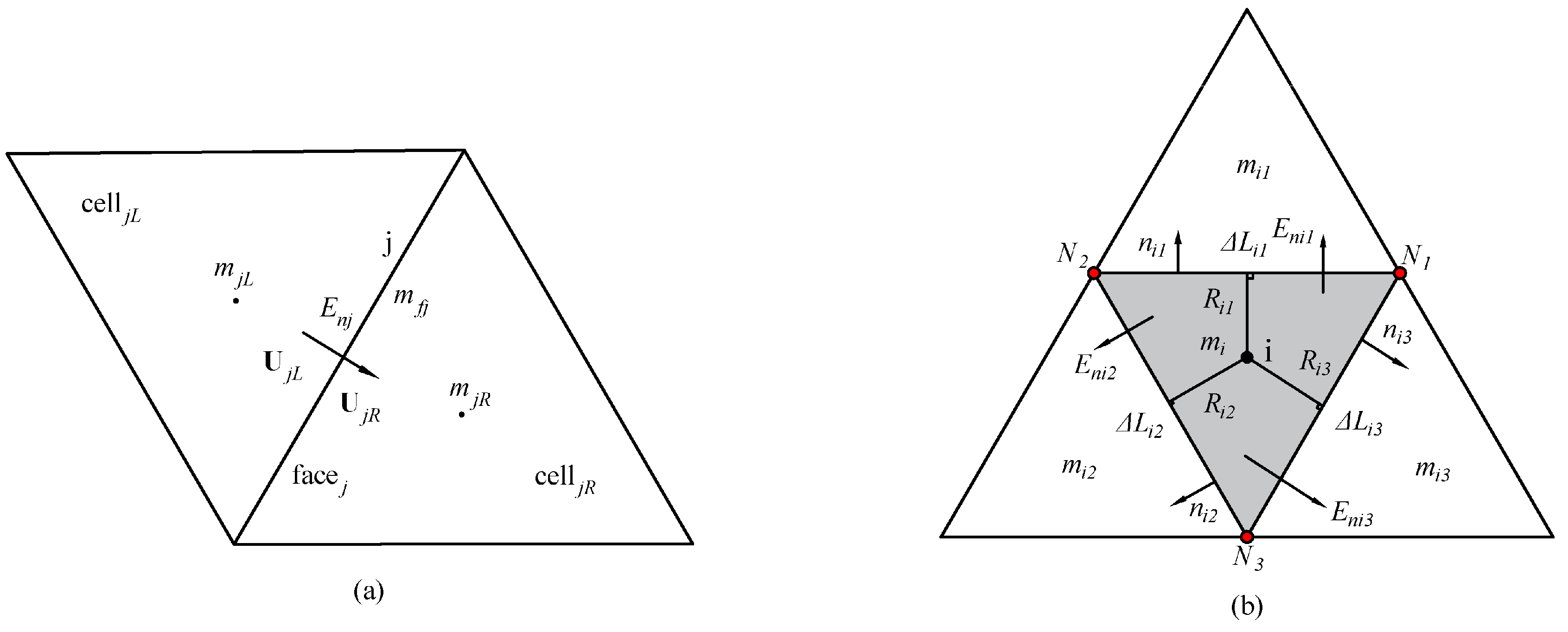
The numerical algorithm employed in this study utilizes the finite volume method to discretize the governing equations of shallow water dynamics. The computational domain is divided into triangular cells, and the equations are integrated over each cell to ensure conservation of mass and momentum. Figure 2 presents sketches of triangular meshes, comprising (a) a face (j) and its two neighboring cells (celljL and celljR); (b) an internal cell (mi) and its three neighboring cells. As mentioned below, the physical parameters shown in Figure 2 will be determined. At the nodes, bed elevations are first determined. The arithmetic average of the three component node elevations is used to calculate the bed elevation for a given cell, and this value is updated during the simulation. The cell center is where other physical characteristics are specified. If needed, the inverse distance interpolation method is employed to derive physical variables at the nodes. To enhance computational efficiency, the local time step (LTS) technique is utilized, allowing each computational cell to use the maximum permissible time step rather than adhering to a globally determined minimum time step (GTS) [22,26,27,28,29,30]. Additionally, GPU parallel acceleration is employed to improve computational efficiency further [27,31,32,33,34,35,36,37].
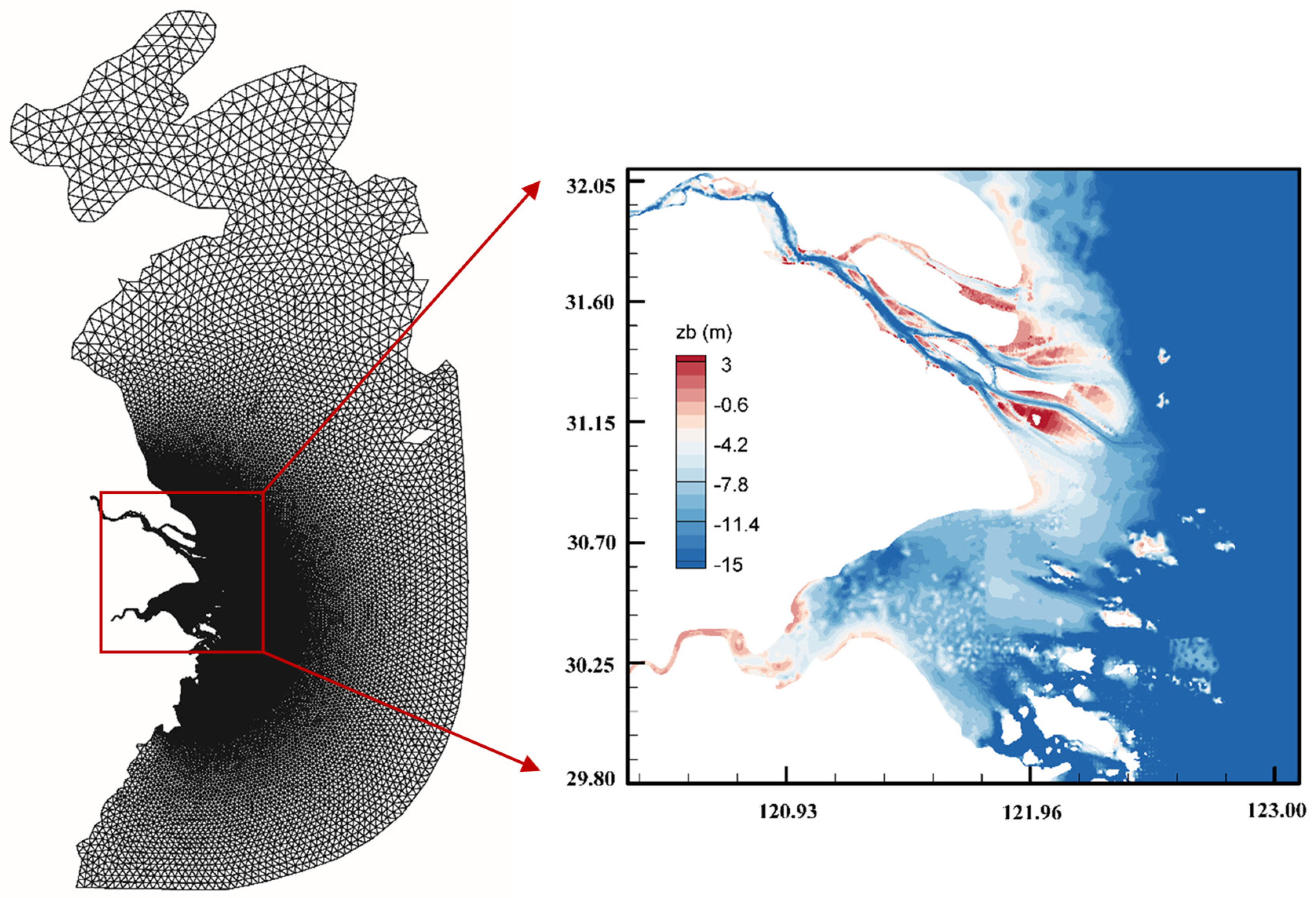
The model calculation area is illustrated in Figure 3, with a longitude range of  117.6524 °   E ~ 127.3857 °   E , and a latitude range of approximately  25.4775 °   N ~ 40.9230 °   N . As depicted in Figure 3, an unstructured triangular mesh has been generated in this study using SMS (The Surface Water Modeling System) [38,39,40]. This grid model is specifically designed to accommodate the intricate topographic shorelines of the Yangtze River estuary, Hangzhou Bay, and the Qiantang River. The grid is locally refined in the nearshore and estuarine areas to capture the complex topography. Specifically, the minimum grid size in the Yangtze River estuary is 15 m, particularly near the island embankments and the deep-water channel project. Additionally, the grid is locally refined up to 80 m in areas such as the Yangtze River estuary and the confluence with Hangzhou Bay. This approach ensures that both coarse and fine grid resolutions are used to balance computational efficiency and accuracy. The model consists of 119,108 grid nodes and 233,397 grid cells, ensuring a high level of detail in the simulation.

2.3. Model Parameter Settings

The following are the established boundary conditions for the model: The Yangtze River’s upper reaches are considered an open boundary, and their salinity is set at zero. The measured flow from the Datong station serves as the boundary condition. Similarly, the upper reaches of the Qiantang River are also considered an open boundary, characterized by minimal runoff and sand content, which exerts almost no influence on the hydrodynamics of the Yangtze River estuary, given the constant flow rate of 1000 m3/s. Additionally, the sand content is set to 0, while the salinity at the offshore boundary is fixed at 35 ppt. The tidal processes at each boundary point are determined using the tidal wave model, TPXO, as the offshore boundary condition. Water level fluctuations impact the inner continental shelf’s curved offshore open boundary, mainly taking into account the subtidal effects of M2, N2, K2, S2, Q1, K1, P1, O1, MF, MM, M4, MS4, and MN4.
The initial conditions for the model calculations were established with a cold start, setting water level and flow velocity to 0. When the water depth was equal to or greater than 0.3333 m, the roughness was determined using the formula 0.01 + 0.01/h. Conversely, if the water depth fell below 0.3333 m, a fixed roughness value of 0.04 was applied [41]. The sediment was divided into 10 grain size groups (0.0025, 0.0065, 0.012, 0.0235, 0.0465, 0.0685, 0.0875, 0.1125, 0.1875, and 0.375 mm) based on the bottom sand measured data in the Yangtze River estuary in January 2016. With a Courant number of 0.9, the time step was calculated for the local time step model. The critical water depth was defined as 0.01 m, and the model operated under dynamic boundary conditions.

2.4. Computational Efficiency

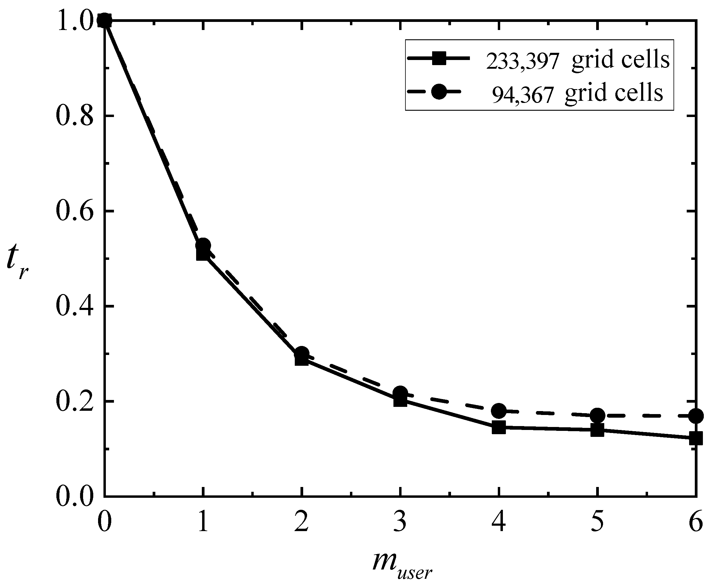
Numerical simulation accuracy is greatly influenced by mesh resolution; however, high-resolution meshes frequently result in a large increase in computation, which puts accuracy and computing efficiency at odds. This work introduces local time step (LTS) approaches and GPU acceleration to address this issue. Using two grid quantities (94,367 and 233,397), this study investigates how well these methods work to increase computational efficiency. This study determines the relative duration of running the model for an hour with various grid numbers in order to more intuitively assess the model’s efficiency improvement. Table 1 and Figure 4 demonstrate how the model run’s efficiency dramatically increases with muser value. The term “muser” refers to the hierarchical level parameter in the local time-stepping (LTS) framework, which quantifies the discretization scale multiplier for adaptive time-step allocation. Specifically, it determines the power-of-two multiple by which each computational cell’s local time step is scaled relative to the global minimum time step, ensuring compliance with the CFL stability condition while optimizing computational efficiency. The term “tr” refers to the relative efficiency, that is, the ratio of the running time under different GPU + LTS scenarios to that under the GPU-only scenario. The efficiency of running 94,367 grid cells increases from 53.353 s to 9.068 s when LTS is set to 5, while the efficiency of running 233,397 grid cells increases from 574.481 s to 80.517 s, or nearly six times. However, the increase in model running efficiency significantly slows down after muser ≥ 3. The efficiency of LTS is also impacted by the total number of grid cells; it is evident that the efficiency is comparatively improved, and the acceleration effect increases with the number of grid cells. As a result, LTS is more useful in complex scenarios involving a large number of grids and plays a larger role when there are more grids and the grid situation is more complicated.

3. Quantitative Accuracy

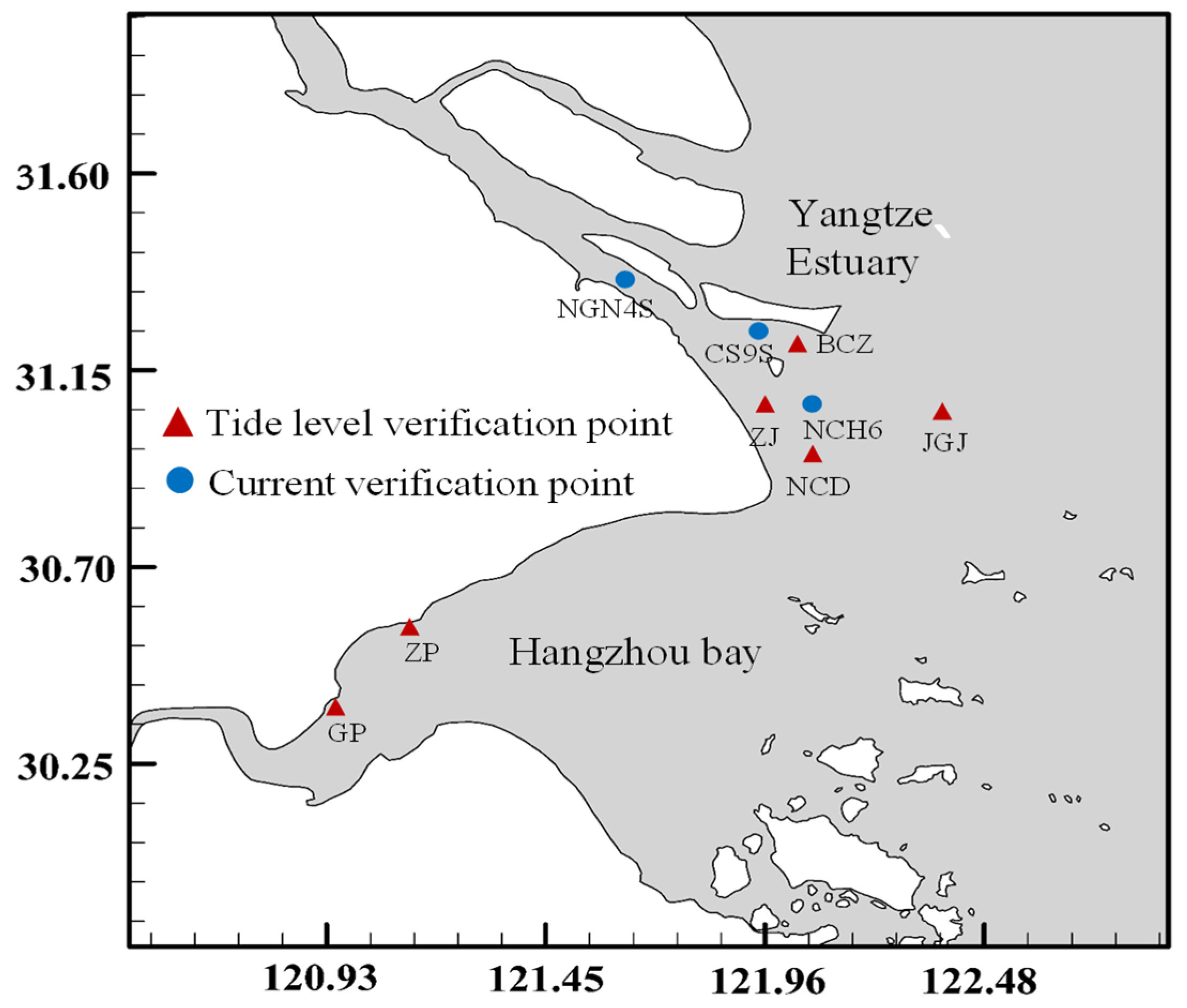
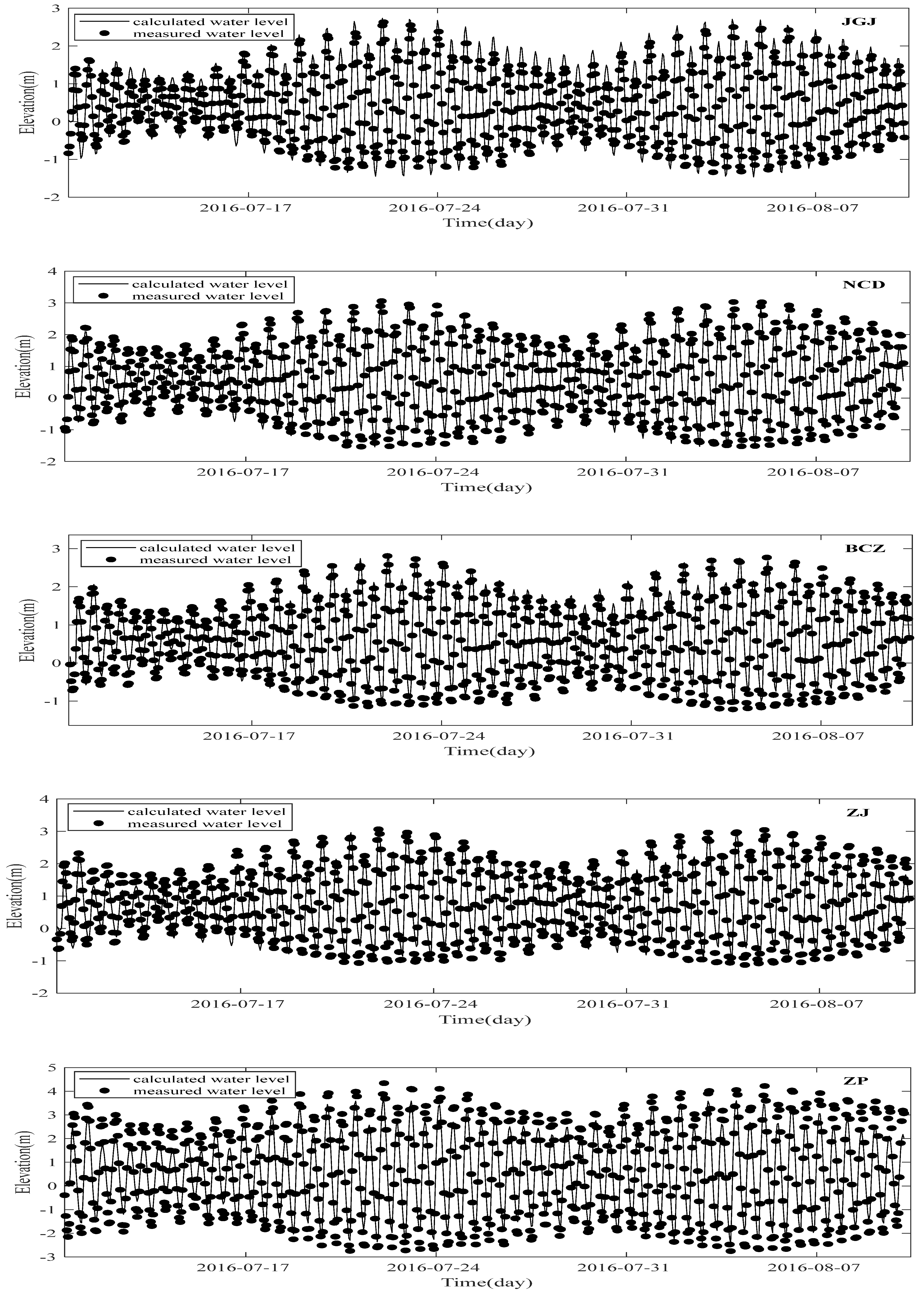
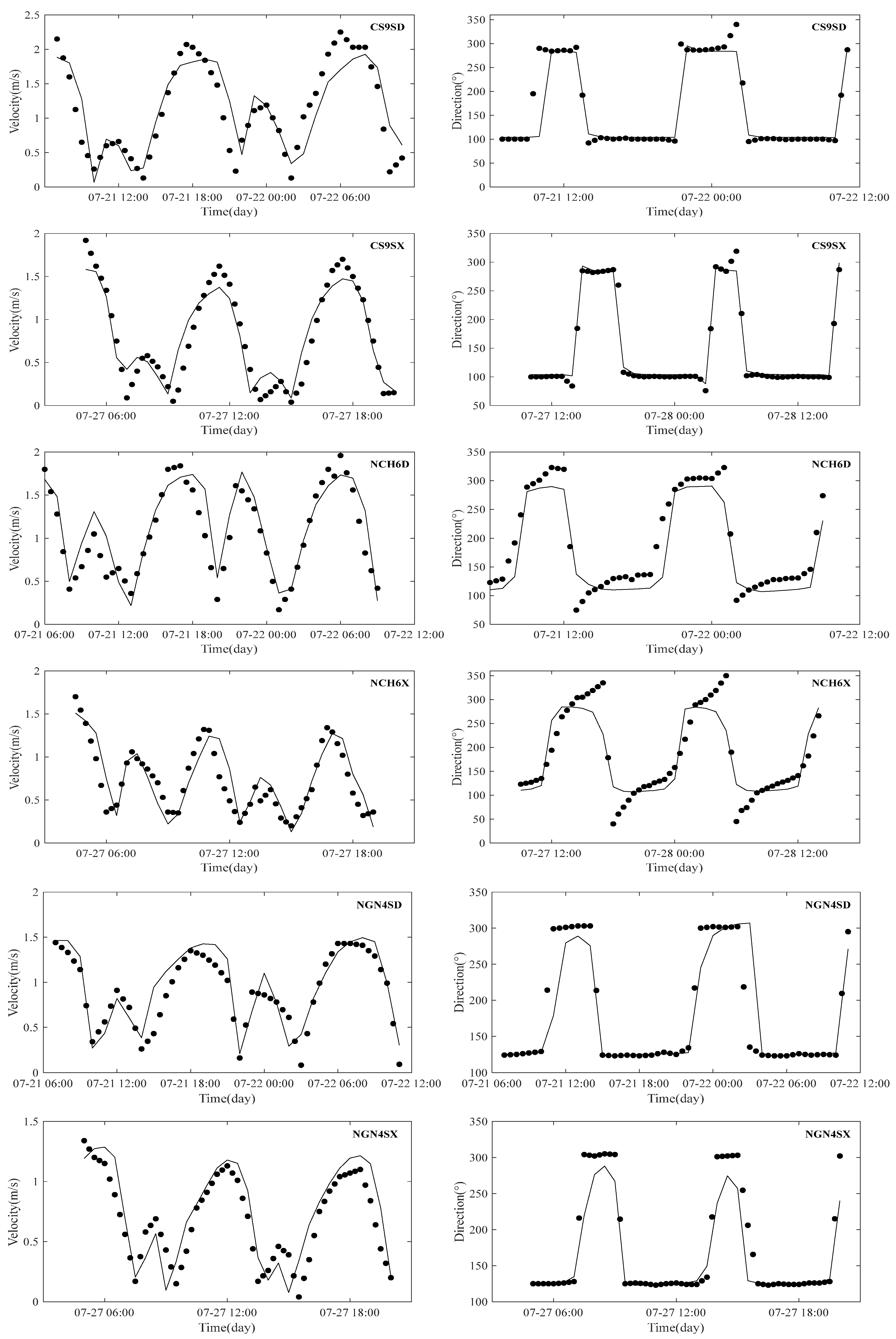
Between 10 July and 10 August 2016, the Yangtze River estuary and Hangzhou Bay underwent hydrodynamic validation. Tidal levels were measured at seven stations: Ji Gu Jiao (JGJ), South Trough East (BCZ), North Trough Middle (NCD), Zhong Jun (ZJ), Gan Pu (GP), and Zha Pu (ZP). Three tidal sites were selected for validation during the spring tide on 21 July 2016, from 7:00 to 11:00, and the neap tide on 27 July 2016, from 10:00 to 16:00. Figure 5 illustrates the locations of these sites. In this study, two parameters are introduced to rigorously quantify the performance of the proposed model: the Root Mean Square Error (RMSE), as expressed in Equation (6), and the Sum of Squares (SS), detailed in Equation (7) [42]. Figure 6 displays a comparison of the simulated and observed water levels, showing that the calculated outcomes correlate well with the actual data. The comparison between the actual and simulated tidal direction and velocity is shown in Figure 7.
The root mean squared error is calculated as follows:
R M S E = [ 1 N i = 1 N ( M i O i ) 2 ] 1 / 2
The technical score SS uses the following equation to assess the simulation validation results:
S S = 1 i = 1 N ( M i O i ) 2 i = 1 N ( O i O ¯ ) 2
where  M i  is the simulated result;  O i  is the observation result;  O ¯  is the mean value of the observation data; L is the number of observed data. The values were divided into four levels according to the size of the SS value to determine whether the model is reliable:  S S > 0.65  is “excellent”;  0.65 S S > 0.5  is “good”;  0.5 S S > 0.2  is “medium”; and  S S < 0.2  is “poor” [43].
The RMSE and SS statistics for these simulations at various stations are compiled in Table 2. Since the SS obtained for both water levels and tidal currents at the site were more significant than 0.65, the simulations were all rated as “excellent” according to the technical rating scale for SS. There exists a strong correlation between the computed and observed tidal levels, suggesting that the model effectively simulates the tidal level changes across the seven stations. Overall, the simulation results are promising, as the simulated flow velocity aligns well with the trends observed in the measured flow velocity, and the simulated direction matches the observed direction closely. However, the simulated values fall short of capturing the complexities of the flow field, as evidenced by the validation curve. This discrepancy arises from the fact that the flow field observed in the field is more intricate than the computational results. Various factors that cannot be fully captured during the modeling process, such as topography and hydrometeorology, influence the actual flow field. Consequently, the factors accounted for do not precisely represent the real situation. Overall, it can be concluded that the computational results provide a more accurate reflection of the flow dynamics, effectively simulating the key characteristics of tidal levels and currents in the study area, thereby meeting the objectives of this paper. In other words, the hydrodynamic model developed here can more accurately represent the actual conditions within the Hangzhou Bay area of the Yangtze River estuary.
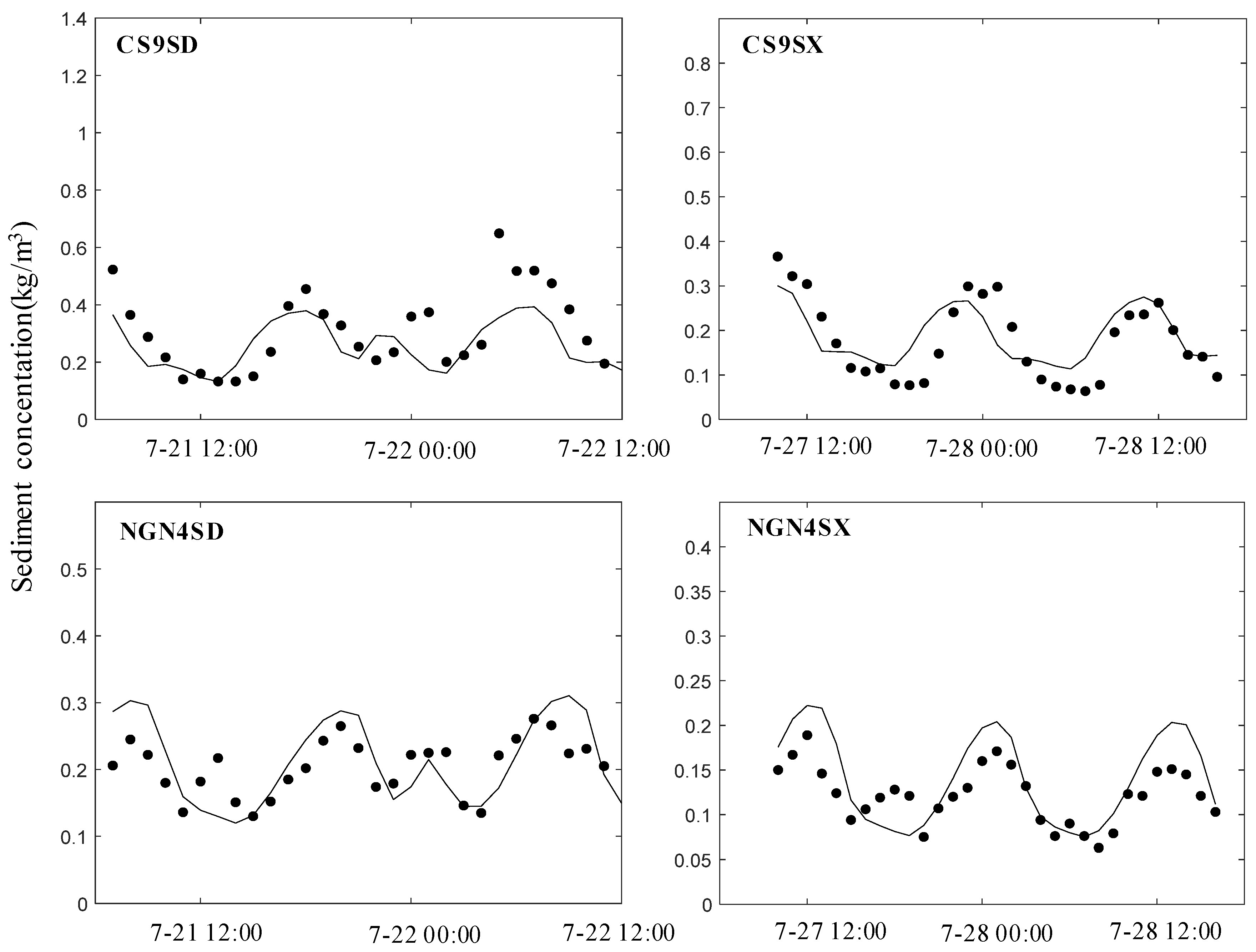
The model sediment concentration validation time was also selected during the spring tide on 21 July 2016, from 7:00 to 11:00, and the neap tide on 27 July 2016, from 10:00 to 16:00. Two validation measurement points, CS9S and NGN4S, were selected to verify the comparison between the sediment concentration and the measured values, and the comparison of the sediment concentration is shown in Figure 8. From the validation results, the trend of change between the simulated values and the measured values of each validation point is consistent, and the magnitude of the values is also in the same order of magnitude. On the whole, the model can better reflect the change of sediment and can be used to study the sediment transport law in the region.

4. Generalized Model and Case Settings

4.1. Adjacent Estuary Idealized Model

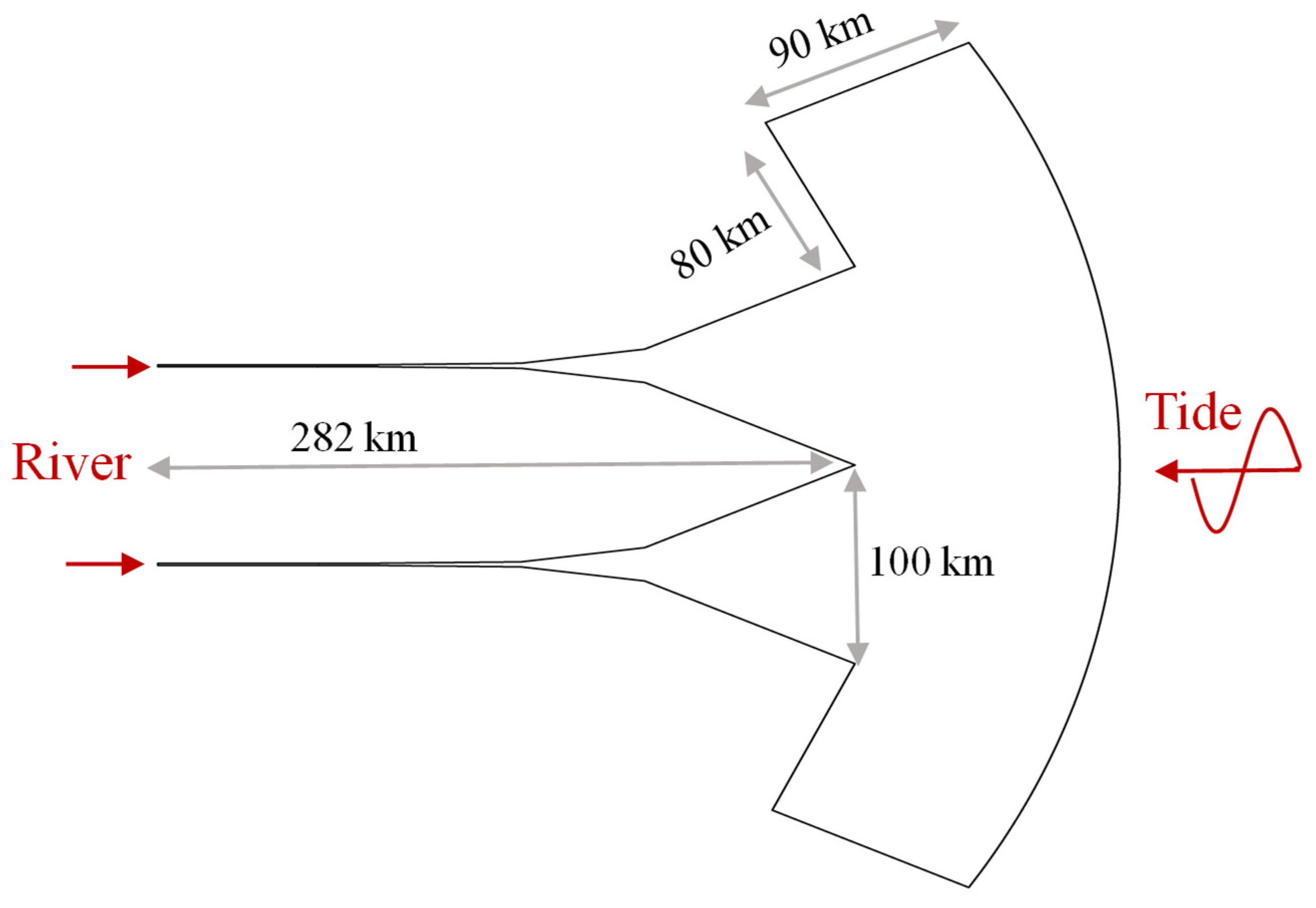
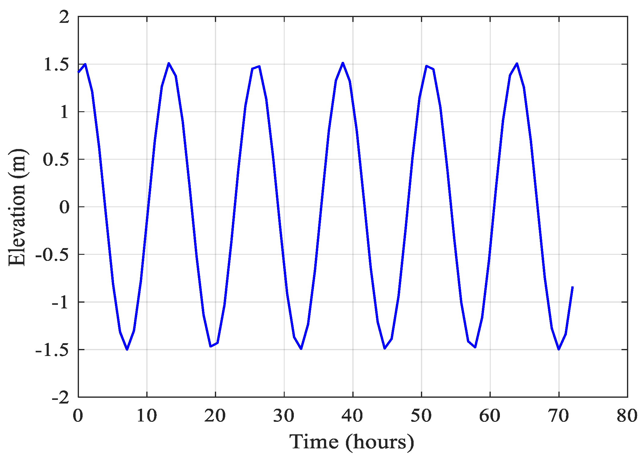
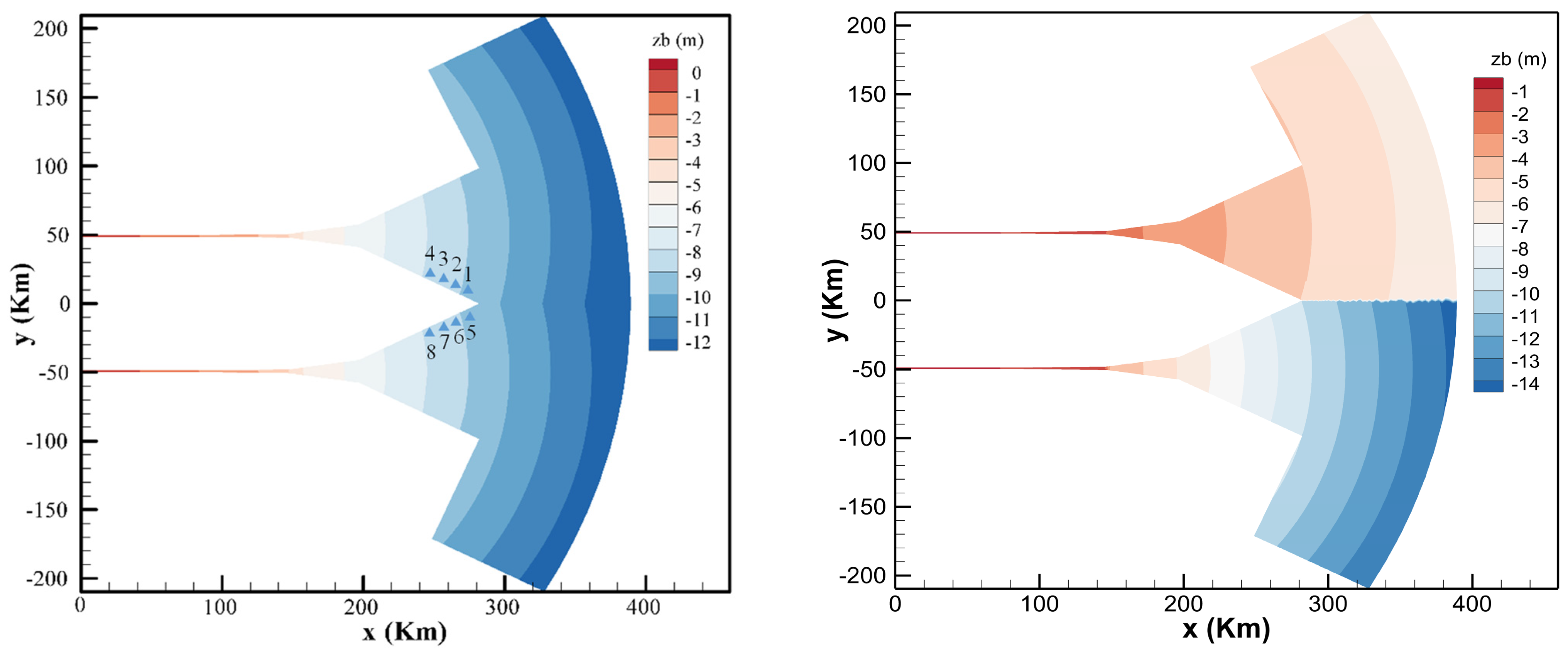
To systematically investigate the influence of the Coriolis force on adjacent estuarine water level differences, a generalized double-trumpet-shaped estuary model was developed. In this study, the estuary system is conceptualized as an idealized model featuring two adjacent estuaries, with a schematic representation provided in Figure 9 [44]. The estuary mouth width is set at 100 km. The open sea boundary is forced by the M2 tidal constituent, characterized by a tidal period of 12.42 h (see Figure 10). Figure 11 provides a detailed representation of the symmetrical and asymmetrical topographical features of the adjacent estuaries, along with the specific sites that were the focus of the study. The topographic elevation progressively descends from 0 m to −12 m along the longitudinal profile, with the water surface level maintained at 0 m. The baseline simulation scenario adopts a discharge rate of 10,000 m3/s (representing dry season conditions in the Yangtze River estuary) and a prescribed tidal range of 3 m. There are 28,615 grid nodes and 55,208 grid cells.

4.2. Case Condition Settings

There are notable seasonal fluctuations in freshwater discharge in the Yangtze Estuary. Three distinct flow regimes are revealed by an analysis of multi-decadal discharge records from the Datong Station: the intermediate season (30,000 m3/s), the dry season (10,000 m3/s), and the flood season (60,000 m3/s). This study first looks at hydrodynamic variations with and without the Coriolis force’s impacts using an actual model of the Yangtze Estuary and Hangzhou Bay. This is followed by the development of an adjacent idealized estuary model, which includes a constant Qiantang River discharge of 950 m3/s and four Yangtze discharge scenarios (10,000, 30,000, 60,000, and 80,000 m3/s) [44]. Table 3 provides a summary of the computational case configurations. Case studies 1 and 2 evaluate how the Coriolis force affects real-world hydrodynamics. On the other hand, case studies 3 through 9 investigate the effects of different Coriolis force coefficients and hemispheres on distributions and differences in tidal levels. The impact of varying discharge is examined in case studies 10 through 13, with particular attention to the effect of the discharge on tidal levels. Lastly, case studies 13 and 14 examine the impacts in different topographic settings.

5. Results

5.1. Effect of the Coriolis Force on Hydrodynamics in Actual Models

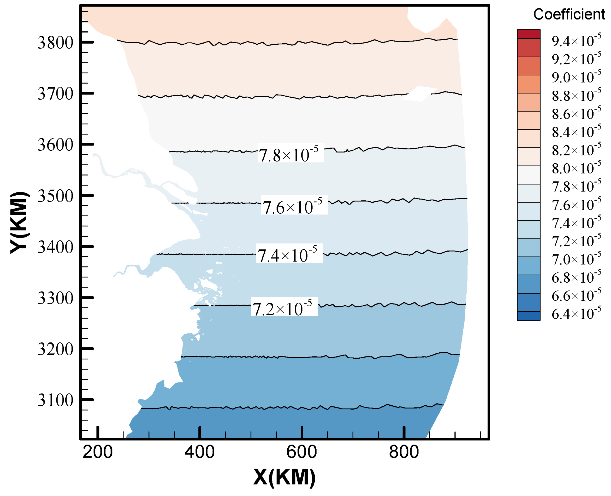
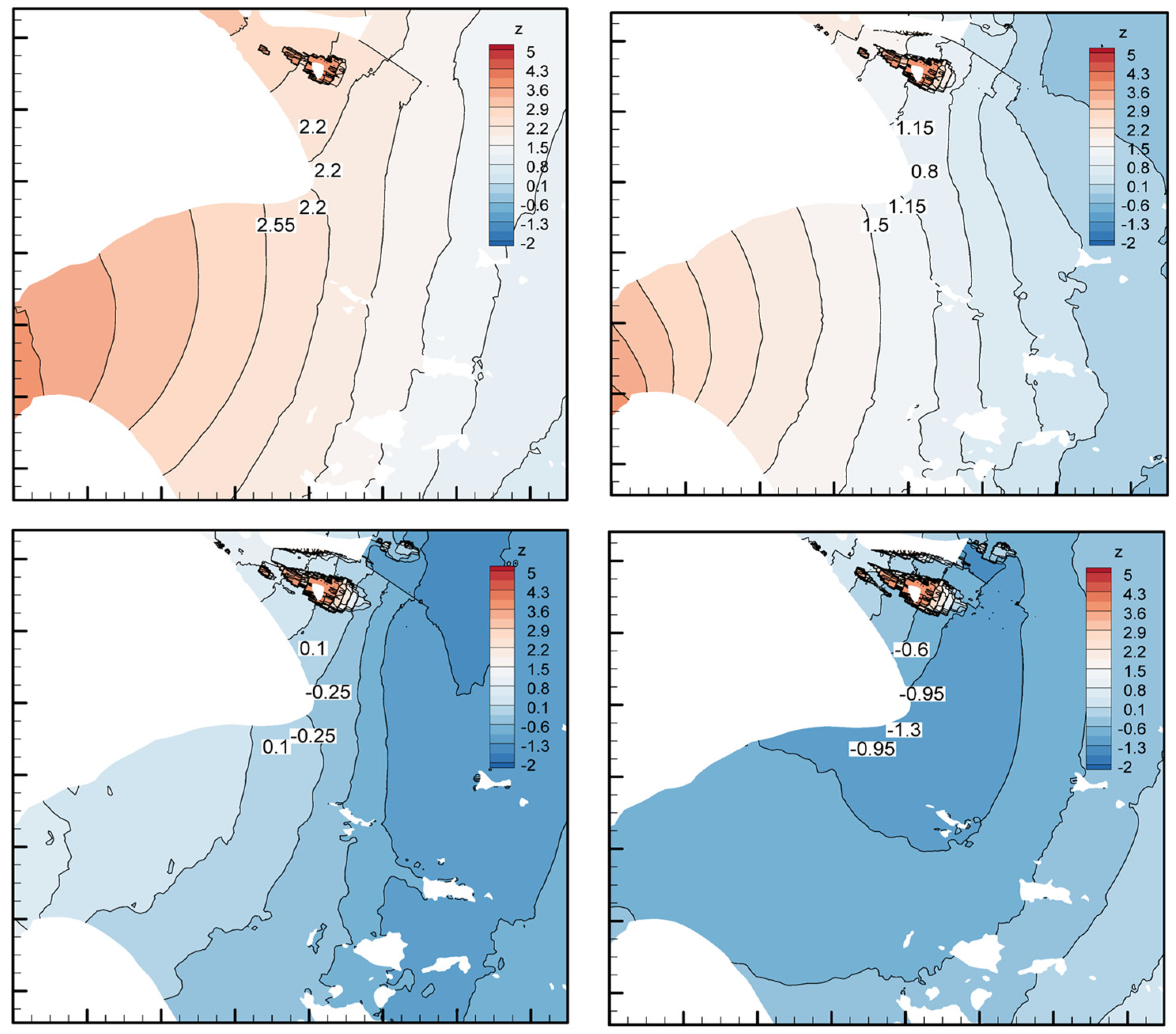
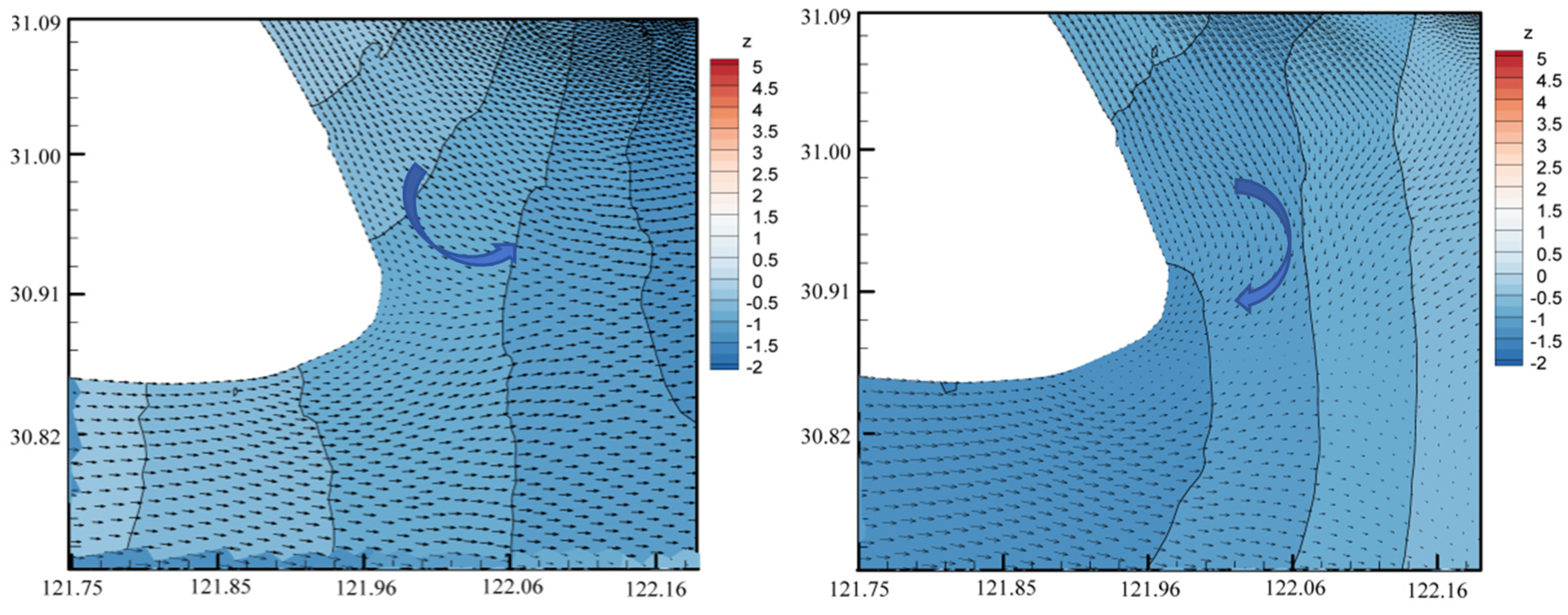
This subsection will focus on the results obtained from the actual model, which is designed to simulate the real-world conditions of the Yangtze River estuary and Hangzhou Bay. The discussion will include the observed hydrodynamic variations, sediment exchange patterns, and the impact of the Coriolis force on tidal level differences. For the sake of examining arithmetic examples 1 and 2, the main entrance of the Yangtze River mouth into Hangzhou Bay is the Nanhui mouth channel. Figure 12 shows that the coefficient of force is  7.6 × 10 5  near the entrance of the Yangtze River and  7.4 × 10 5  near Hangzhou Bay. Latitude affects the Coriolis parameter; the higher the latitude, the greater the Coriolis parameter, and vice versa. Figure 13 shows the striking disparities between the results of running the program for 11.5 days, 11.6668 days, 11.8334 days, and 12 days during spring tide when the Coriolis force is taken into account, as opposed to values without it. According to measurements, this gradient is roughly between 0 and 0.35 m. In the scenario when the Coriolis effect is included, the water level gradient between Hangzhou Bay and the Yangtze River estuary rises to roughly 0.35 to 0.7 m. This illustrates how the water level gradients at the ZJ and LCG stations are greatly impacted by the Coriolis force’s existence or absence. Sediment transport is impacted by the Coriolis effect, which raises the water level gradient between Hangzhou Bay and the Yangtze River mouth. While the Coriolis force is one of the key drivers of these processes, we acknowledge that other factors, such as wind stress, river discharge, and topographic effects, also contribute to the observed patterns.
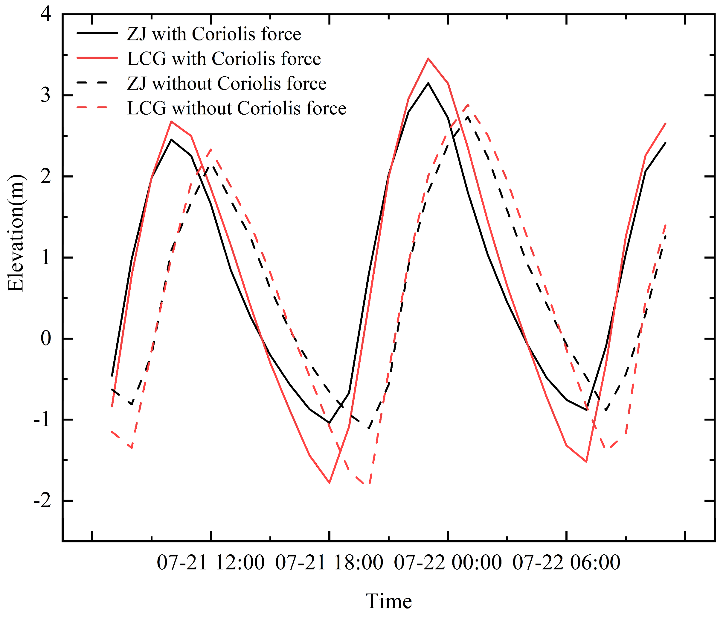
Two key stations, LCG and ZJ, were chosen for analysis, and their latitudes along with Coriolis parameters are presented in Table 4. Comparative tidal level plots for these stations during spring tide conditions were created. As shown in Figure 14, the Coriolis force results in high tidal levels occurring approximately two hours earlier at individual stations, thereby inducing a phase shift across the entire tidal curve. The Coriolis force alters the propagation dynamics of a rotating tidal wave system by introducing a lateral deflection of the current motion, resulting in differences in the propagation velocity of the leading edge of the wave at different latitudes.
The tidal dynamical processes in Hangzhou Bay are also impacted by the Coriolis force. Figure 15 shows the current flow patterns close to Nanhui Shoal, where Hangzhou Bay and the Yangtze River estuary converge. The model comparison shows different flow patterns: when the Coriolis force is absent, estuarine currents go southeast, in accordance with the tidal effect. However, the flow vector is redirected toward Hangzhou Bay due to a notable rightward deflection caused by Coriolis forces. An interchange of water and sediment occurs from the Yangtze River mouth to Hangzhou Bay during the ebb tide as a result of the Coriolis effect in the Northern Hemisphere deflecting the current to the right of its direction of motion.
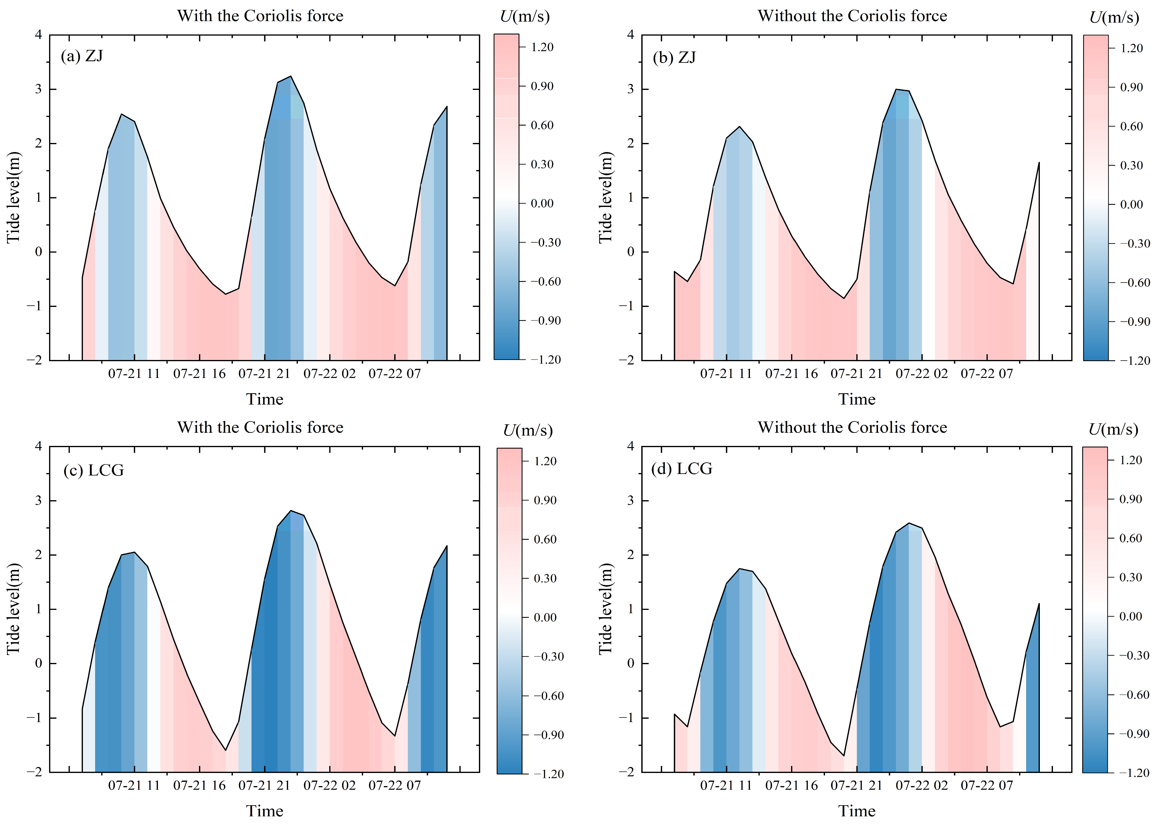
Figure 16 shows that the effect of the Coriolis force on the flow velocity distribution and water–sand exchange was characterized by significant spatial differentiation. In LCG, the Coriolis force tends to increase the flow velocity at high tide (u < 0), while the flow velocity at low tide (u > 0) tends to decrease. This asymmetric regulation causes the high tide duration to be shortened by approximately 1.2 h and the dominant flow duration to be prolonged at low tide, hence creating a notable tidal asymmetry. The ZJ station exhibits the opposite pattern, with the flow velocity at high tide being comparatively weaker and the Coriolis force increasing the peak flow velocity at low tide. By altering the flow velocity distribution and tidal dynamics properties, the Coriolis force has a substantial impact on tidal asymmetry and its function in regional water–sand exchange.
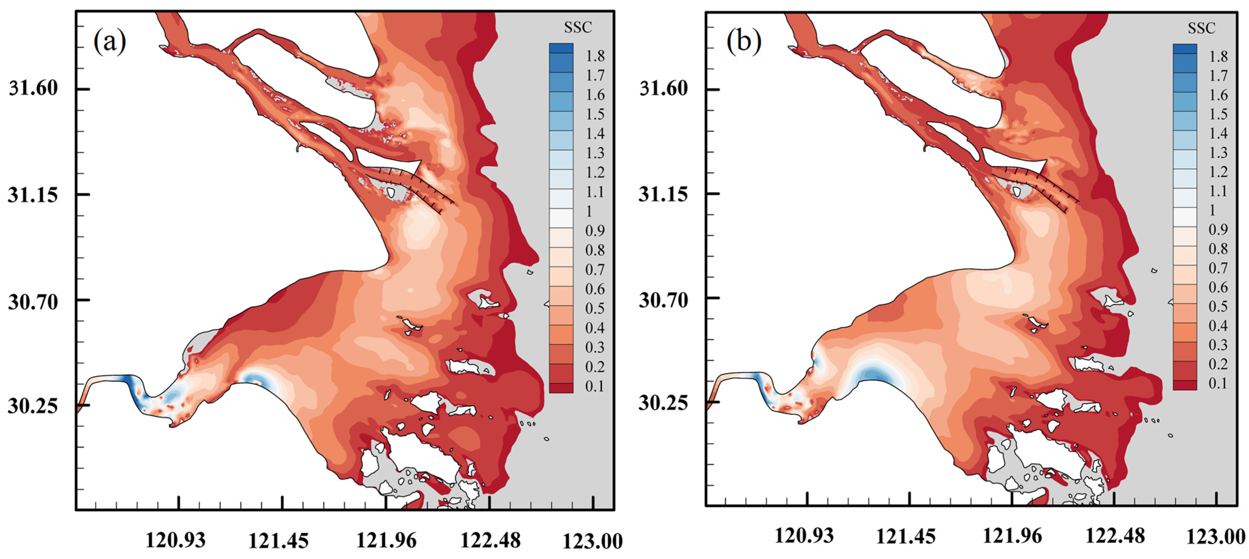
The water–sediment transport characteristics of the Yangtze River estuary and Hangzhou Bay region change significantly when considering the effects of the Coriolis force. Specifically, the Coriolis force deflects the freshwater plume of the Yangtze River towards the southern coast (in the direction of Nanhui District) during its seaward transport. This deflection leads to an increase in suspended sediment transport to the north side of Hangzhou Bay, contributing to the region of high sediment concentration offshore of Nanhui District (see Figure 17).

5.2. Analysis of the Arithmetic Results of the Idealized Generalized Model

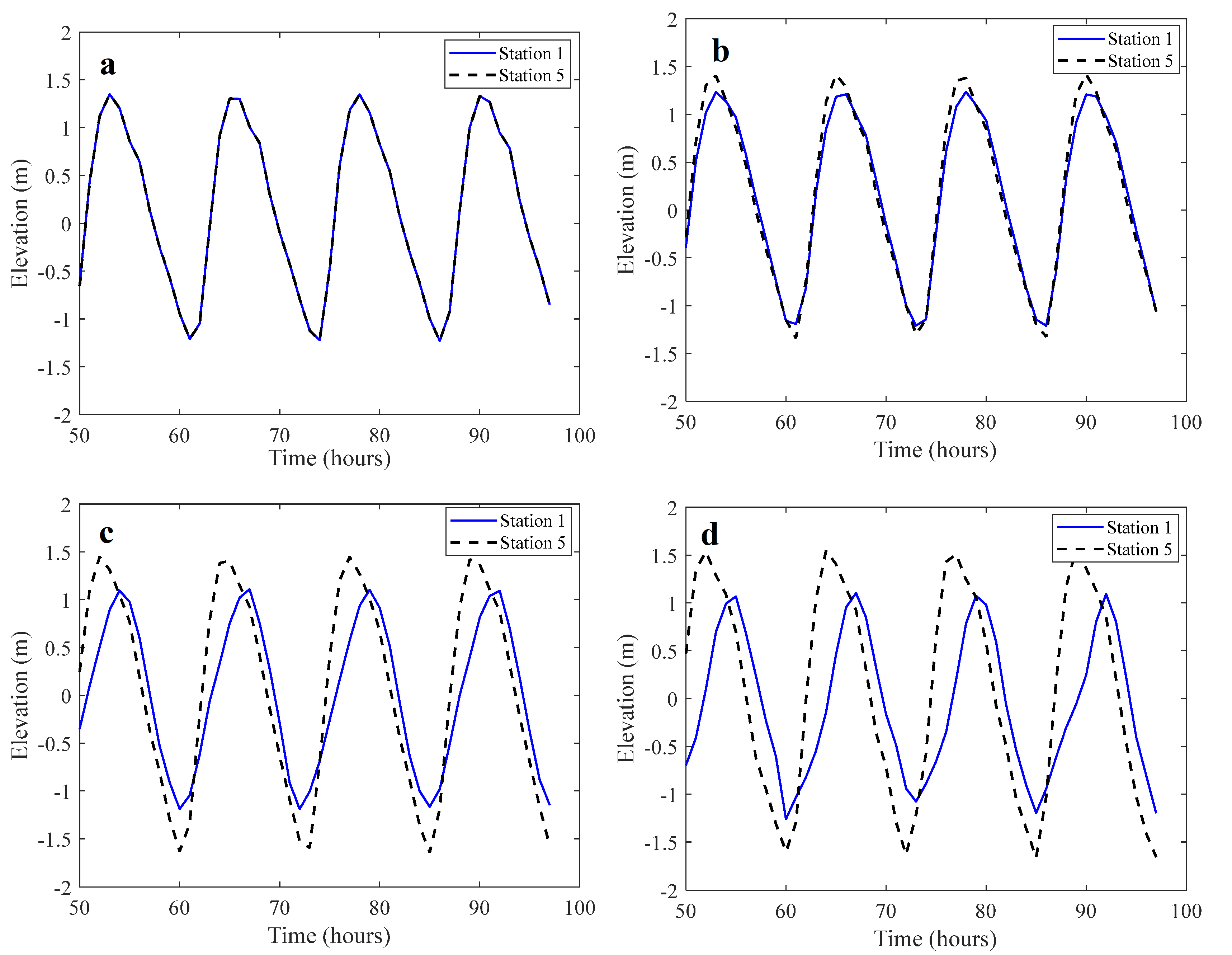
This subsection will present the results from the generalized model, which is used to explore the effects of varying Coriolis forces, flow conditions, and topographical features. Cases 3 through 9 investigate the impact of various Coriolis force coefficients on the water level difference between adjacent estuarine stations 1 and 5 (see Figure 18). This analysis is conducted under base conditions, specifically a flow of 10,000 m3/s during the dry season and a tidal range of 3 m. The analysis was structured around sets of latitudes at 30° N, 60° N, 85° N, 30° S, 60° S, and 85° S. In the absence of the Coriolis force, the tidal level difference between Stations 1 and 5 is minimal, approaching zero. As the Coriolis coefficient increases, a distinct tidal level difference emerges between the two stations. A larger Coriolis coefficient enhances the Coriolis effect, resulting in more pronounced flow deflection and greater phase differences. The increased phase difference intensifies the rightward deflection of tidal wave propagation (in the Northern Hemisphere), thereby amplifying the tidal phase discrepancy between the adjacent estuaries and forming a stronger lateral water level gradient. During flood and ebb tides, spatiotemporal variations in the inter-estuary water level difference drive lateral compensatory flows, which enhance cross-estuary water exchange and promote the transport of suspended sediment.
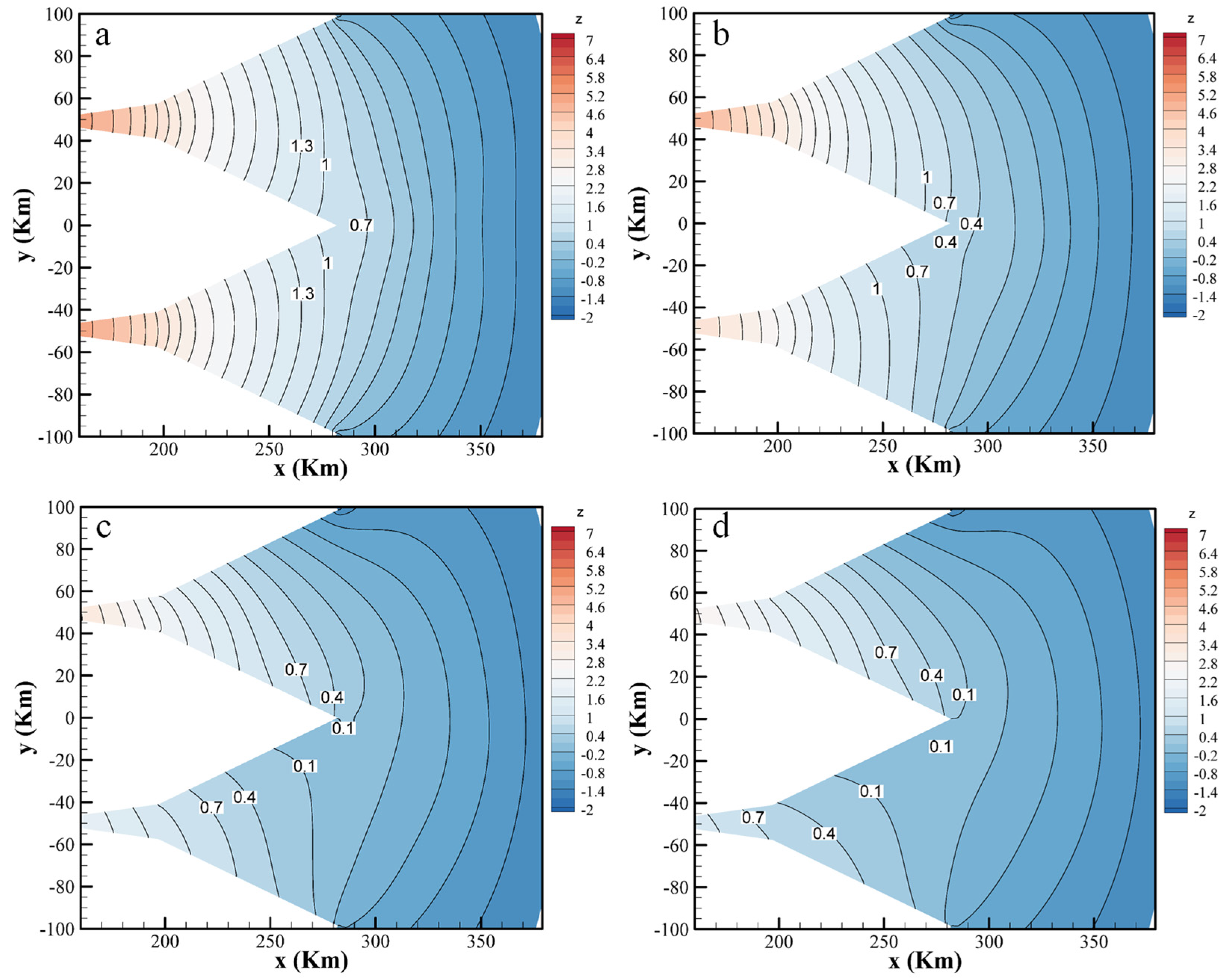
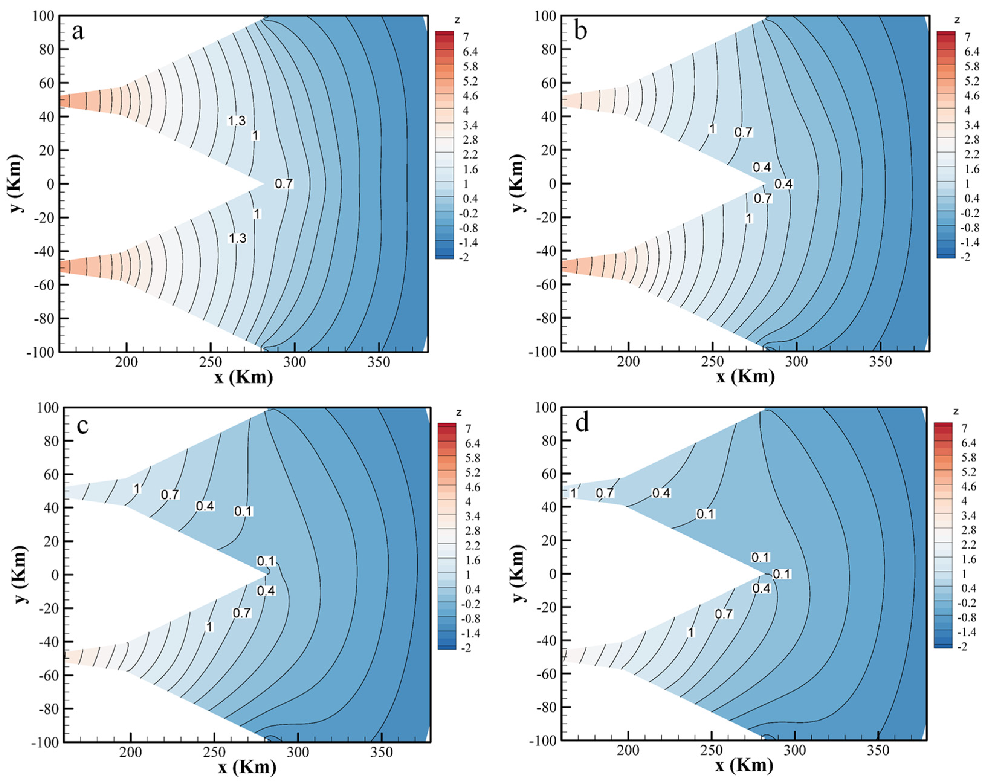
In reference to Figure 19 (Northern Hemisphere) and Figure 20 (Southern Hemisphere), which illustrate the tidal level distributions under various Coriolis force coefficients, the results presented pertain to the ebb tide at 288,000 s.
In the absence of Coriolis force, it is evident that the distribution of tidal levels at the confluence of nearby estuaries is entirely symmetrical, with no variation in tidal levels. The tidal level distribution on the north and south banks of a single estuary is likewise symmetrical. At ebb tide in the Northern Hemisphere, the Coriolis force will cause the current to deflect to the right side of the direction of movement, causing the water level of the north bank of the estuary to fall and the water level of the south bank to rise [45,46,47,48,49]. This is reflected in the nearby estuaries, where the tide level of the south bank of the upper estuary is higher than that of the north bank of the lower estuary, resulting in the tidal level difference, as illustrated in Figure 18. The water level on the north bank of the estuary rises, and the water level on the south bank falls at low tide in the Southern Hemisphere due to the Coriolis force, which deflects the current to the left of the direction of motion. This phenomenon is mirrored in the neighboring estuaries, where the tidal level on the north bank of the next estuary is higher than that on the south bank of the preceding estuary (see Figure 20). The distribution of the tidal level between the confluence of two estuaries becomes increasingly asymmetrical, and the asymmetry of the tidal level distribution within a single estuary becomes more noticeable as the Coriolis force coefficient and its influence grows. This indicates that the distribution of water levels and the difference in water levels across adjacent estuaries are influenced by the Coriolis force.
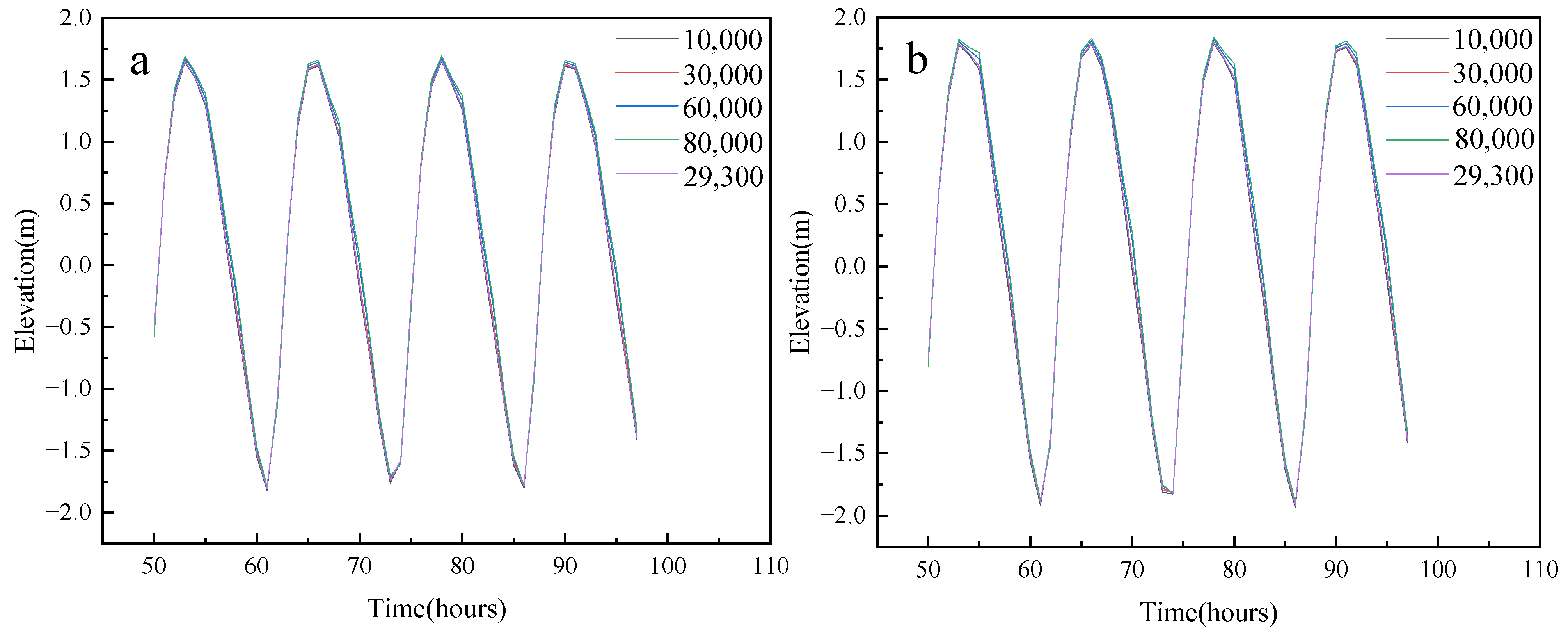
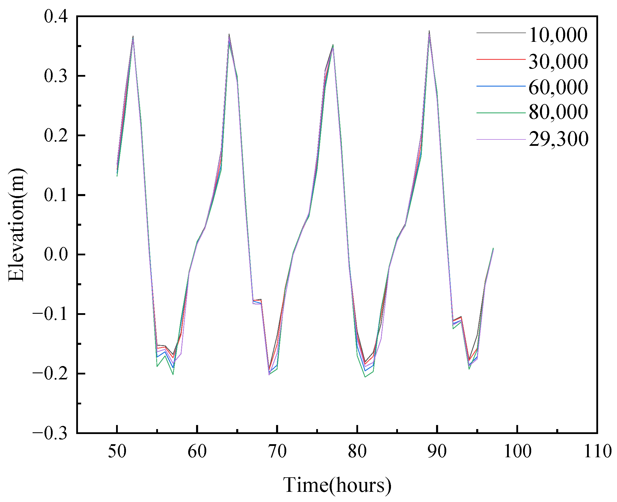
Cases 4, 10, 11, 12, and 13 investigate discharge impacts under constant Coriolis parameter ( f = 2 w sin 30 , Ω = 7.29 × 10⁻⁵ rad/s) and 3 m tidal range modulation. Hydrometric analysis reveals limited stage variation between dry seasons (Q = 10,000 m3/s), wet seasons (Q = 60,000 m3/s), average flow, and extreme flooding (Q = 80,000 m3/s) at the monitoring stations 1 and 4 (see Figure 21). Notably, both high and low tidal levels exhibit discharge-dependent amplification, attributable to river-tide hydrodynamic interactions. Importantly, the discharge does not alter the differences in tidal levels between adjacent estuaries. As depicted in Figure 22, the tidal level differences between Site 5 and Site 1 remain essentially consistent across varying discharge conditions. The results show that changes in river flow have a limited effect on tidal levels and a negligible effect on the water level gradient in nearby estuaries.
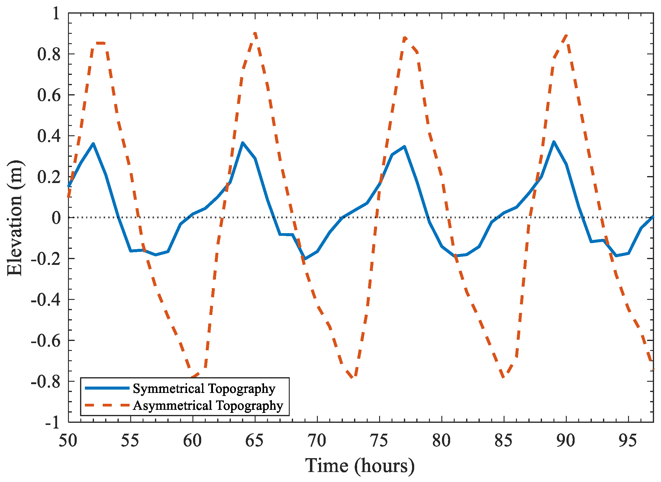
Case studies 13 and 14 explore the impact of varying topographic conditions on the tidal level differences observed between adjacent estuaries. It is noted that when the topography of both estuaries is identical, the tidal level difference between Site 5 and Site 1 remains relatively small, measuring less than 0.4 m. In contrast, under asymmetric topographic conditions, where the upstream estuary features an entrance depth of −5 m, the tidal level difference between Site 5 and Site 1 increases to 0.8 m (see Figure 23). This clearly demonstrates that topography differences have a significant influence on tidal level gradients in neighboring estuaries.

6. Conclusions

To clarify the crucial function of the Coriolis force in controlling sediment–water exchange between the Yangtze River estuary and Hangzhou Bay (HZB), this study uses a GPU-accelerated shallow water model with local time-stepping (LTS). By accelerating tidal phases by around two hours and intensifying tidal asymmetry, Earth’s rotation creates lateral water level gradients (0.35–0.7 m), according to numerical simulations that combine idealized and realistic estuary designs. The long-held theory that the majority of the sediment in HZB comes from the YRE is supported mechanistically by these dynamics, which propel slope currents during late ebb tides and enable southern sediment movement from the YRE’s northern bank into HZB. Furthermore, idealized modeling shows that hemispheric contrasts reverse tidal level distribution patterns, whereas latitude-dependent Coriolis coefficients improve sediment exchange, with greater coefficients enhancing flow deflection and phase differences. Despite the fact that changes in river discharge (10,000–60,000 m3/s) have little effect on cross-estuary gradients, topographic asymmetry greatly increases tidal level variations (up to 0.8 m). The GPU-accelerated model has demonstrated its effectiveness in replicating intricate estuary processes by being validated against field data with high accuracy (SS scores rated “excellent” for tidal levels).
However, it is important to recognize the limitations of our study. While the Coriolis force is a critical factor, globally, estuarine sedimentation is primarily driven by fluvial sediment discharge from upstream sources, an aspect not explicitly considered. Additionally, tidal asymmetry, which is characterized by disparities in the intensities of flood and ebb tides, plays a dominant role in sediment transport. Our analysis does not fully explore these fundamental aspects, which are essential for a comprehensive understanding of estuarine sedimentary processes.
Despite these limitations, these results provide a solid framework for comprehending estuarine sediment dynamics in a changing world and highlight the need to include Earth’s rotating impacts into coastal management methods. By advancing our understanding of the mechanisms driving sediment–water exchange, this work contributes to the development of more effective management strategies for estuarine and coastal environments. Future research should aim to integrate the effects of tidal asymmetry into models to better understand estuarine sediment transport processes. Specifically, future studies should aim to perform the following:
  • Quantify the relative contributions of tidal asymmetry and the Coriolis force to sediment transport in the Yangtze River estuary and Hangzhou Bay system.
  • Investigate the long-term impacts of sea-level rise and anthropogenic activities on tidal asymmetry and sediment dynamics.

Author Contributions

Conceptualization, P.H.; Methodology, J.T. (Jia Tang) and P.H.; Software, J.T. (Jia Tang), Z.Z. and Z.F.; Validation, J.T. (Jia Tang); Investigation, J.T. (Jia Tang); Resources, P.H., Z.Z., J.T. (Junyu Tao) and A.J.; Writing—original draft, J.T. (Jia Tang); Writing—review & editing, J.T. (Jia Tang), P.H. and L.D. All authors have read and agreed to the published version of the manuscript.

Funding

This research is supported by the National Natural Science Foundation of China (No. 12172331), the Zhejiang Natural Science Foundation (LGEZ25E090003), the Zhoushan Municipal Bureau of Science and Technology, Zhoushan Marine Research Center of Zhejiang University (2023C51004), and the HPC Center OF ZJU (ZHOUSHAN CAMPUS).

Data Availability Statement

Simulations results are available on request from the corresponding author.

Conflicts of Interest

The authors declare no conflicts of interest.

References

  1. Chen, J.Y.; Chen, S.L.; Ding, P.X. Sediment transport pathways in the nearshore waters of Nan-huizui, Yangtze River Estuary. Resour. Environ. Yangtze Basin. 2001, 10, 166–172. (In Chinese) [Google Scholar]
  2. Yang, S.L.; Milliman, J.D.; Li, P.; Xu, K. 50,000 dams later: Erosion of the Yangtze River and its delta. Glob. Planet. Change 2011, 75, 14–20. [Google Scholar] [CrossRef]
  3. Dai, Z.; Fagherazzi, S.; Mei, X.; Gao, J. Decline in suspended sediment concentration delivered by the Changjiang (Yangtze) River into the East China Sea between 1956 and 2013. Geomorphology 2016, 268, 123–132. [Google Scholar] [CrossRef]
  4. Li, P.; Yang, S.; Milliman, J.D.; Xu, K.; Qin, W.; Wu, C.; Chen, Y.; Shi, B. Spatial, temporal, and human-induced variations in suspended sediment concentration in the surface waters of the Yangtze estuary and adjacent coastal areas. Estuaries Coasts 2012, 35, 1316–1327. [Google Scholar] [CrossRef]
  5. Dai, Z.; Liu, J.T.; Xie, H.; Shi, W. Sedimentation in the Outer Hangzhou Bay, China: The influence of Changjiang sediment load. J. Coast. Res. 2014, 30, 1218–1225. [Google Scholar] [CrossRef]
  6. Dai, Z.; Liu, J.T.; Wei, W.; Chen, J. Detection of the Three Gorges Dam influence on the Changjiang (Yangtze River) submerged delta. Sci. Rep. 2014, 4, 6600. [Google Scholar] [CrossRef] [PubMed]
  7. Brown, J.M. Davies A G. Flood/ebb tidal asymmetry in a shallow sandy estuary and the impact on net sand transport. Geomorphology 2010, 114, 431–439. [Google Scholar] [CrossRef]
  8. Wang, B.; Zhu, J.; Li, L. Analysis of the dynamic causes of flood-ebb asymmetry in the Yangtze River Estuary. Acta Oceanol. Sin. 2011, 33, 19–27. (In Chinese) [Google Scholar]
  9. Pan, C.; Zheng, J.; Chen, G.; He, C.; Tang, Z. Spatiotemporal variations and causes of tidal characteristics in Hangzhou Bay. Ocean Eng. 2019, 37, 11. (In Chinese) [Google Scholar]
  10. Suh, S.W.; Lee, H.Y.; Kim, H.J. Spatio-Temporal Variability of Tidal Asymmetry Due to Multiple Coastal Constructions along the West Coast of Korea. Estuar. Coast. Shelf Sci. 2014, 151, 336–346. [Google Scholar] [CrossRef]
  11. Suh, S.W. Tidal Asymmetry and Energy Variation Due to Sea-Level Rise in a Macro Tidal Bay. J. Coast. Res. 2016, 75, 765–769. [Google Scholar] [CrossRef]
  12. Ji, X.; Huang, L.; Zhang, W.; Yao, P. On the Mechanism behind the Variation of the Tidal Current Asymmetry in Response to Reclamations in Lingding Bay, China. J. Mar. Sci. Eng. 2022, 10, 951. [Google Scholar] [CrossRef]
  13. Feng, X.; Feng, H. On the Role of Anthropogenic Activity and Sea-Level-Rise in Tidal Distortion on the Open Coast of the Yellow Sea Shelf. J. Geophys. Res. Oceans 2021, 126, e2020JC016583. [Google Scholar] [CrossRef]
  14. Li, J. Study on sediment transport patterns in the Nanhui tidal flat of the Yangtze River Estuary. Acta Oceanol. Sin. 1990, 75–82. (In Chinese) [Google Scholar]
  15. Cao, P.; Yan, S. Suspended sediment front in the Yangtze River Estuary and its impact on material transport. J. East China Norm. Univ. (Nat. Sci.) 1996, 85–94. (In Chinese) [Google Scholar]
  16. Kong, J.; Ye, R.; Xue, X.; Zhou, Y. Impact of Nanhui East Shoal on sediment exchange between the Yangtze Estuary and Hangzhou Bay. Waterw. Port. 2009, 30, 77–81. (In Chinese) [Google Scholar]
  17. Huang, G. Study on Water and Sediment Exchange and Transport Characteristics Between the Yangtze Estuary and Hangzhou Bay. Ph.D. Thesis, East China Normal University, Shanghai, China, 2007. (In Chinese). [Google Scholar]
  18. Huang, J.; Zhu, J.; Su, J.; Han, X.; Cai, L. Suspended sediment exchange between the Changjiang Estuary and Hangzhou Bay and their key driving mechanisms. Estuar. Coast. Shelf Sci. 2024, 305, 108876. [Google Scholar] [CrossRef]
  19. Sassi, M.G.; Hoitink, A.J.F. River flow controls on tides and tide-mean water level profiles in a tidal freshwater river. J. Geophys. Res. Oceans 2013, 118, 4139–4151. [Google Scholar] [CrossRef]
  20. Guo, L.; van der Wegen, M.; Roelvink, J.A.; He, Q. The role of river flow and tidal asymmetry on 1D estuarine morphodynamics. J. Geophys. Res. Earth Surf. 2014, 119, 2315–2334. [Google Scholar] [CrossRef]
  21. Guo, L.; van der Wegen, M.; Roelvink, D.; He, Q. Exploration of the impact of seasonal river discharge variations on long-term estuarine morphodynamic behavior. Coast. Eng. 2015, 95, 105–116. [Google Scholar] [CrossRef]
  22. Hu, P.; Han, J.; Li, W.; Sun, Z.; He, Z. Numerical investigation of a sandbar formation and evolution in a tide-dominated estuary using a hydro-morphodynamic model. Coast. Eng. J. 2018, 60, 466–483. [Google Scholar] [CrossRef]
  23. Hou, J.; Liang, Q.; Simons, F.; Hinkelmann, R. A 2D well-balanced shallow flow model for unstructured grids with novel slope source term treatment. Adv. Water Resour. 2013, 52, 107–131. [Google Scholar] [CrossRef]
  24. Liang, Q.; Marche, F. Numerical resolution of well-balanced shallow water equations with complex source terms. Adv. Water Resour. 2009, 32, 873–884. [Google Scholar] [CrossRef]
  25. Zhang, R.; Xie, J.; Wang, M.; Huang, J. River Sediment Dynamics; Water Resources and Electric Power Press: Beijing, China, 1989. (In Chinese) [Google Scholar]
  26. Crossley, A.J.; Wright, N.G. Time accurate local time stepping for the unsteady shallow water equations. Int. J. Numer. Meth. Fluids 2005, 48, 775–799. [Google Scholar] [CrossRef]
  27. Dazzi, S.; Vacondio, R.; Dal Palù, A.; Mignosa, P. A local time stepping algorithm for GPU-accelerated 2D shallow water models. Adv. Water Resour. 2018, 111, 274–288. [Google Scholar] [CrossRef]
  28. Dazzi, S.; Maranzoni, A.; Mignosa, P. Local time stepping applied to mixed flow modelling. J. Hydraul. Res. 2016, 54, 145–157. [Google Scholar] [CrossRef]
  29. Hu, P.; Lei, Y.; Han, J.; Cao, Z.; Liu, H.; He, Z. Computationally efficient modeling of hydro-sediment-morphodynamic processes using a hybrid local time step/global maximum time step. Adv. Water Resour. 2019, 127, 26–38. [Google Scholar] [CrossRef]
  30. Hu, P.; Lei, Y.; Han, J.; Cao, Z.; Liu, H.; He, Z.; Yue, Z. Improved local time step for 2D shallow-water modeling based on unstructured grids. J. Hydraul. Eng. 2019, 145, 06019017. [Google Scholar] [CrossRef]
  31. Hu, P.; Zhao, Z.; Ji, A.; Li, W.; He, Z.; Liu, Q.; Li, Y.; Cao, Z. A GPU-accelerated and LTS-based finite volume shallow water model. Water 2022, 14, 922. [Google Scholar] [CrossRef]
  32. Vacondio, R.; Dal Palù, A.; Ferrari, A.; Mignosa, P.; Aureli, F.; Dazzi, S. A non-uniform efficient grid type for GPU-parallel shallow water equations models. Environ. Model. Softw. 2017, 88, 119–137. [Google Scholar] [CrossRef]
  33. Lacasta, A.; Morales-Hernández, M.; Murillo, J.; García-Navarro, P. An optimized GPU implementation of a 2D free surface simulation model on unstructured meshes. Adv. Eng. Softw. 2014, 78, 1–15. [Google Scholar] [CrossRef]
  34. Brodtkorb, A.R.; Sætra, M.L.; Altinakar, M. Efficient shallow water simulations on GPUs: Implementation, visualization, verification, and validation. Comput. Fluids 2012, 55, 1–12. [Google Scholar] [CrossRef]
  35. Lacasta, A.; Morales-Hernández, M.; Murillo, J.; García-Navarro, P. GPU implementation of the 2D shallow water equations for the simulation of rainfall/runoff events. Environ. Earth Sci. 2015, 74, 7295–7305. [Google Scholar] [CrossRef]
  36. Castro, M.J.; Ortega, S.; de la Asunción, M.; Mantas, J.M.; Gallardo, J.M. GPU computing for shallow water flow simulation based on finite volume schemes. Comptes Rendus Mec. 2010, 339, 165–184. [Google Scholar] [CrossRef]
  37. de la Asunción, M.; Castro, M.J. Simulation of tsunamis generated by landslides using adaptive mesh refinement on GPU. J. Comput. Phys. 2017, 345, 91–110. [Google Scholar] [CrossRef]
  38. Zhang, M.; Zhang, H. SMS Hydrodynamic Software. Waterw. Harbor. 2006, 1, 57–59. (In Chinese) [Google Scholar]
  39. Scientific Software Group Surface Water Modeling System (SMS). In Encyclopedia of Hydrological Sciences; John Wiley & Sons, Ltd.: Hoboken, NJ, USA, 2006; pp. 154–196. [CrossRef]
  40. Wu, Z.; Xu, X. Modeling of the Yangtze River Estuary-Hangzhou Bay Waters Based on SMS. China Water Transp. (Second. Half Mon.) 2013, 13, 125–126. (In Chinese) [Google Scholar]
  41. Dou, X.; Li, L.; Dou, G. Study on the Total Sediment Mathematical Model of the Yangtze River Estuary. J. Hydraul. Eng. Water Resour. Res. 1999, 2, 32–41. (In Chinese) [Google Scholar]
  42. Warner, J.C.; Geyer, W.R.; Lerczak, J.A. Numerical modeling of an estuary: A comprehensive skill assessment. J. Geophys. Res. Oceans 2005, 110, C05001. [Google Scholar] [CrossRef]
  43. Allen, J.I.; Somerfield, P.J.; Gilbert, F.J. Quantifying uncertainty in high-resolution coupled hydrodynamic-ecosystem models. J. Mar. Syst. 2007, 64, 3–14. [Google Scholar] [CrossRef]
  44. Guo, Y.; Wu, X.; Pan, C.; Zhang, J. Numerical simulation of the tidal flow and suspended sediment transport in the Qiantang Estuary. J. Waterw. Port Coast. Ocean Eng. 2012, 138, 192–202. [Google Scholar] [CrossRef]
  45. Yu, D. Analysis on Impact of the Coriolis Forces on Flow in the Yangtze River Estuary. In Proceedings of the Third Chinese-German Joint Symposium on Coastal and Ocean Engineering National, Tainan, Taiwan, 8–16 November 2006. [Google Scholar]
  46. Osadchiev, A.; Alfimenkov, I.; Rogozhin, V. Influence of the Coriolis force on spreading of river plumes. Remote Sens. 2023, 15, 3397. [Google Scholar] [CrossRef]
  47. Li, M.; Chen, Z.; Yin, D.; Chen, J.; Wang, Z.; Sun, Q. Morphodynamic characteristics of the dextral diversion of the Yangtze River mouth, China: Tidal and the Coriolis force controls. Earth Surf. Process. Landf. 2011, 36, 641–650. [Google Scholar] [CrossRef]
  48. Xie, D.; Gao, S.; Wang, Z.B.; Pan, C.; Wu, X.; Wang, Q. Morphodynamic modeling of a large inside sandbar and its dextral morphology in a convergent estuary: Qiantang Estuary, China. J. Geophys. Res. Earth Surf. 2017, 122, 1553–1572. [Google Scholar] [CrossRef]
  49. Yang, Z.; Cheng, H.; Li, J. Nonlinear advection, Coriolis force, and frictional influence in the South Channel of the Yangtze Estuary, China. Sci. China Earth Sci. 2015, 58, 429–435. [Google Scholar] [CrossRef]
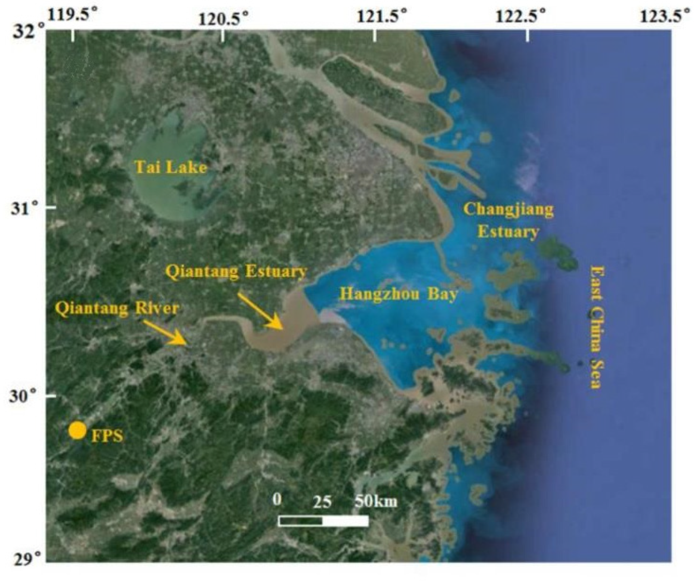
Figure 1. Location of Qiantang Estuary.
Water 17 01011 g001
Figure 2. Sketches of the unstructured triangular meshes: (a) a face (j) and its two neighboring cells (celljL and celljR); (b) an internal cell (mi) and its three neighboring cells.
Water 17 01011 g002
Figure 3. Initial bed topography of computational domain, unstructured mesh for Yangtze Estuary and Hangzhou Bay cases.
Water 17 01011 g003
Figure 4. Comparison of efficiency in different muser cases.
Water 17 01011 g004
Figure 5. Stations for the available measured data.
Water 17 01011 g005
Figure 6. Verification of water level (dots denote the observed data; lines represent the simulation data).
Water 17 01011 g006aWater 17 01011 g006b
Figure 7. Verification of depth-averaged tidal velocity and direction (dots denote the observed data; lines represent the simulation data).
Water 17 01011 g007
Figure 8. Verification of the sediment concentration (dots denote the observed data; lines represent the simulation data).
Water 17 01011 g008
Figure 9. Schematic of the generalized model.
Water 17 01011 g009
Figure 10. Tide level profile of M2 at the offshore boundary.
Water 17 01011 g010
Figure 11. Schematic of the topography of the generalized model.
Water 17 01011 g011
Figure 12. Coefficients of Coriolis force with latitude.
Water 17 01011 g012
Figure 13. Comparison of tidal levels at Nanhui Shoal without and with the Coriolis force ((left) Coriolis force excluded; (right) Coriolis force included).
Water 17 01011 g013aWater 17 01011 g013b
Figure 14. Comparison of the LCG and ZJ with and without Coriolis force.
Water 17 01011 g014
Figure 15. Comparative visualization of ebb–tide current fields: Coriolis-inhibited scenario (left) versus Coriolis-active dynamics (right).
Water 17 01011 g015
Figure 16. Distribution of flow velocity clouds for ZJ and LCG with and without Coriolis force. ((a) ZJ with the Coriolis force; (b) ZJ without the Coriolis force; (c) LCGwith the Coriolis force; (d) LCG without the Coriolis force).
Water 17 01011 g016
Figure 17. Distribution of the sediment concentration with and without Coriolis force ((a) Coriolis force excluded; (b) Coriolis force included).
Water 17 01011 g017
Figure 18. Effects of different Coriolis coefficients on Stations 1 and 5 ((a) without; (b) 30° N; (c) 60° N; (d) 85° N).
Water 17 01011 g018
Figure 19. Planar distribution of tidal levels under different Coriolis coefficients ((a) without; (b) 30° N; (c) 60° N; (d) 85° N).
Water 17 01011 g019
Figure 20. Planar distribution of tidal levels under different Coriolis coefficients ((a) without; (b) 30° S; (c) 60° S; and (d) 85° S).
Water 17 01011 g020
Figure 21. Tidal stage plot of station 1 and station 4 under different discharge conditions ((a) station 1; (b) station 4).
Water 17 01011 g021
Figure 22. Tidal level differences between Site 5 and Site 1 under varying flow conditions.
Water 17 01011 g022
Figure 23. Tidal level differences between Site 5 and Site 1 under different topographic conditions.
Water 17 01011 g023
Table 1. The calculation time of different cases.
PC
Platform
Methodmuser94,367 Grid Cells233,397 Grid Cells
Time/strTime/str
PC:
GTX 1660
GPU053.3531.00574.4811.00
GPU + LTS128.1430.53292.9860.51
215.9910.30166.1130.29
311.5490.22116.6080.20
49.5970.1883.5380.15
59.0680.1780.5170.14
69.0280.1770.3840.12
Table 2. Model performance (SS and RMSE) in simulating hydrodynamics.
StationsHydrodynamicsSSRMSELevel
JGJWater level0.91220.2760 mExcellent
BCZ0.92230.2796 m
NCD0.91440.3714 m
ZJ0.86070.4033 m
ZP0.92390.4642 m
GP0.89980.5314 m
CS9SDTidal current velocity0.79340.2940 m/s
NCH6D0.82650.2097 m/s
NGN4SD0.81980.1667 m/s
CS9SX0.87930.1983 m/s
NCH6X0.77180.1778 m/s
NGN4SX0.74690.1748 m/s
CS9SDTidal current direction0.852534°
NCH6D0.860931°
NGN4SD0.772036°
CS9SX0.981711°
NCH6X0.816138°
NGN4SX0.869526°
Table 3. Case matrix under different operating conditions.
CaseModelBoundary 1
(m3/s)
Boundary 2
(m3/s)
Boundary 3CoriolisTopography
1Actual modelMeasured flow process 1000TPXO modeling process for calculating tide levelsWith (actual)Actual Topography
2Without
3Idealized generalized model10,0003 mWithoutSymmetrical Topography
430° N
560° N
685° N
730° S
860° S
985° S
1030,00030° N
1160,000
1280,000
1329,300950
14Asymmetrical Topography
Table 4. Site Coriolis force coefficient table.
StationLongitudeCoefficient of Force
ZJ31.08950.0000751038
LCG30.81810.0000745131
Disclaimer/Publisher’s Note: The statements, opinions and data contained in all publications are solely those of the individual author(s) and contributor(s) and not of MDPI and/or the editor(s). MDPI and/or the editor(s) disclaim responsibility for any injury to people or property resulting from any ideas, methods, instructions or products referred to in the content.