A Numerical Investigation into the Performance of Bypass Systems During Filling and Air Removal in Partially Drained Pipelines

Abstract

This study presents an elastic one-dimensional numerical model to simulate the filling process of a large-scale, partially drained pipeline with an undulating profile, incorporating bypass systems. The model uses the Method of Characteristics to solve water hammer equations and integrates the Discrete Gas Cavity Model to capture column separation effects. Validation is performed using two experimental test rigs and comparisons with existing numerical models, showing RMSE values between 1.06 and 7.95. The results highlight three key findings: (1) oversized bypasses generate severe transient pressures; (2) effective air management enables higher filling flow rates, significantly reducing filling time; and (3) bypass lines help dampen pressure fluctuations, with a notable drop in $∆H$ from 528 m to 6.8 m occurring in stage b, following the release of trapped air. Additionally, this study challenges the practicality of the AWWA’s recommended pipeline filling velocity limit of 0.3 m/s, showing that strict adherence to this guideline is often unrealistic for large-scale systems. Overall, the findings emphasize the need for a balanced design approach that reduces transient risks while maintaining operational efficiency in large-scale pipelines.

1. Introduction

Filling water and wastewater pipelines presents a significant engineering challenge due to the risk of transient pressure surges, which can cause pipe bursts, joint failures, and operational disruptions. These surges arise from the complex interactions between water and entrapped air during rapid filling. Such interactions may trigger severe pressure oscillations, particularly when air release mechanisms are insufficient [1]. Martin [2] was among the first to identify that when pipelines contain entrapped air pockets, rapid pressurization can result in severe pressure spikes—findings later confirmed through both experimental and numerical studies [3,4,5]. Compressed air pockets amplify pressure levels far beyond the upstream driving force, significantly increasing the likelihood of structural damage [5]. Additionally, incomplete air removal contributes to pressure losses, reduces transmission capacity, and can trigger sudden surges when air is abruptly expelled [6]. Due to these risks, accurate prediction of transient pressures and the optimization of filling strategies—particularly in large-scale pipelines with undulating profiles, where hydraulic column separation influences flow behavior—remain critical for ensuring operational safety and long-term infrastructure reliability.

Air management is considered one of the most effective methods for controlling transient pressures during pipeline filling [7]. Researchers have developed numerical models to improve the prediction of pressure surges caused by air–water interactions. Zhou et al. [5] used the Rigid Column Model to analyze rapid pressurization in pipelines with air pockets, demonstrating reasonable agreement with experimental data. However, this model tends to overestimate pressure surges, particularly in long pipelines with small air volumes [8]. Introducing water column and pipe elasticity has been shown to reduce these overestimations, highlighting the importance of considering elastic effects in transient modeling. One-dimensional models have continued to evolve, with additional elasticity effects improving predictive accuracy [9,10], yet many still struggle to fully capture pressure dissipation over multiple transient cycles. Lee [11] tackled this issue by introducing a thermodynamic correction that accounts for heat exchange between air and water, significantly improving model performance. The Discrete Air Model (DAM), introduced by Feng et al. [8] improved transient pressure prediction, which enhances accuracy by discretizing air pockets and capturing localized pressure fluctuations.

Although 1D models have grown increasingly sophisticated, some researchers have turned to three-dimensional (3D) computational fluid dynamics (CFD) models to achieve more detailed simulations of air–water interactions [12,13,14]. CFD models can capture localized flow features, air pocket deformation, and high-gradient pressure zones with remarkable precision. García-Todolí et al. [15] used CFD techniques to evaluate the intake and expulsion capacity of commercial air valves, demonstrating that, with proper mesh resolution and turbulence modeling, air valve performance can be reasonably predicted under controlled conditions. Paternina-Verona et al. [16] developed a digital twin approach using a 3D OpenFOAM model linked with real-time data, showing that CFD tools can effectively simulate transient air release through valves during pipeline filling. However, despite these promising results, the computational cost of 3D simulations remains prohibitively high, particularly for large-scale transmission pipelines with long and undulating profiles. Moreover, accurately representing complex boundary conditions such as dynamic air valve behavior still presents challenges. Consequently, developing computationally efficient models remains essential for optimizing pipeline filling strategies, mitigating transient pressures, and ensuring the reliability of water infrastructure.

One of the most commonly used air management tools in pipeline systems is the air release valve, particularly during filling and drainage operations. However, improper sizing or placement of these valves may result in inadequate air expulsion, pressure imbalances, or operational failures [17,18]. Ramezani and Karney [18] analytically demonstrated that air cavity formation causes differential acceleration in adjacent water columns. When air is released, these columns may collide violently, inducing severe water hammer pressures. The magnitude of these surges depends on factors like air valve orifice size, valve placement, pipeline length, and profile shape. Zhou et al. [5] examined the influence of air release orifice size on transient pressures during rapid pipeline filling. Their study, which involved a horizontal pipeline with an upstream reservoir and a downstream air release orifice, revealed that larger orifices can intensify water hammer effects. The location of trapped air pockets also plays a critical role, with high-point accumulations exacerbating localized surges, particularly in long or undulating pipelines where transient modeling becomes increasingly complex [19]. Malekpour and Karney [20] further investigated rapid filling in undulating pipelines and found that entrapped air can lead to water column separation at valve locations. Once the air is expelled, the sudden convergence of adjacent water columns generates secondary water hammer pressures, adding another layer of complexity to transient behavior. These findings have been validated through both experimental and numerical studies, reinforcing the challenges associated with air management in pipeline systems [7,21,22].

Another widely used approach to mitigating transient pressures is regulating the filling flow rate. However, no universally accepted computational framework currently determines the optimal rate for different pipeline configurations. In practice, engineers often rely on the American Water Works Association (AWWA) guideline, which suggests a very conservative filling velocity of 0.3 m/s [23]. While this recommendation is widely applied, it is based on simplified assumptions and lacks rigorous validation. Furthermore, strict adherence to this protocol is often impractical, particularly in manually operated pipelines where flow adjustments depend on throttling valves rather than automated control systems. Wang et al. [24] emphasized the importance of bypass systems in balancing pressure mitigation with operational efficiency, yet their effectiveness depends on proper design. Despite their potential, few studies have systematically examined how bypass lines and air valve sizing interact to influence transient pressure behavior.

The aim of this paper is to develop a one-dimensional elastic model that incorporates by-pass and air management strategies in order to simulate transient flow behavior during the filling of large-scale, partially drained pipelines. Unlike previous approaches that often isolate air management or bypass effects, the proposed model simultaneously evaluates their interactions under transient conditions. This integrated treatment enables a more realistic prediction of pressure surges and air release behavior, providing a practical framework for optimizing pipeline filling strategies. The governing equations are constructed by coupling the Method of Characteristics with the Discrete Gas Cavity Model to account for column separation effects. Bypass lines and air valves are incorporated as dynamic boundary conditions to reflect practical system responses. The model is then evaluated through comparisons with both laboratory-scale experiments and two established numerical models. Following validation, the influence of air valve nozzle diameter and bypass pipe size is analyzed to explore their role in pressure regulation. The paper concludes with a summary of key outcomes and implications for real-world pipeline filling strategies.

2. Theoretical Background

The aim of this paper is to develop a one-dimensional elastic model that incorporates bypass and air management strategies in order to simulate transient flow behavior during the filling of large-scale, partially drained pipelines. Unlike previous approaches that often isolate air management or bypass effects, the proposed model simultaneously evaluates their interactions under transient conditions. This integrated treatment enables a more realistic prediction of pressure surges and air release behavior, providing a practical framework for optimizing pipeline filling strategies. The governing equations are constructed by coupling the Method of Characteristics with the Discrete Gas Cavity Model to account for column separation effects. Bypass lines and air valves are incorporated as dynamic boundary conditions to reflect practical system responses. The model is then evaluated through comparisons with both laboratory-scale experiments and two established numerical models. Following validation, the influence of air valve nozzle diameter and bypass pipe size is analyzed to explore their role in pressure regulation. The paper concludes with a summary of key outcomes and implications for real-world pipeline filling strategies.

2.1. Governing Assumptions and Equations

The numerical model is based on the following assumptions [8,24,25]: (1) an elastic one-dimensional formulation is used that accounts for both water compressibility and pipe wall elasticity to enable realistic pressure wave simulation; (2) the friction coefficient is assumed to be a function of the pipe material and remains constant along the pipeline; (3) the air–water interface is assumed to remain perpendicular to the pipe centerline; (4) the compressible entrapped air is assumed to follow a polytropic process with a constant polytropic exponent, ensuring that the air pressure within the air pocket remains uniformly distributed.

The following partial differential equations govern transient flow in pressurized conduit system and are well known as water hammer equations [26,27].

$${\displaystyle \frac{\partial V}{\partial t}}+g{\displaystyle \frac{\partial H}{\partial x}}+{\displaystyle \frac{f}{2D}}\left|V\right|V=0$$

(1)

$${\displaystyle \frac{\partial H}{\partial t}}+{\displaystyle \frac{a^2}{g}}{\displaystyle \frac{\partial V}{\partial x}}=0$$

(2)

where $V$ = velocity, $g$ = gravitational acceleration, $H$ = piezometric head, $D$ = pipe diameter, a = elastic wave speed, g = gravitational acceleration, $f$ = Darcy–Weisbach friction factor, and $x$ and $t$ = distance and time independent variables respectively.

When pipeline pressure drops to vapor pressure, cavitating flow and column separation occur, complicating hydraulic modeling. In such cases, standard transient flow equations alone cannot fully capture system behavior. A widely used approach to address this is the Discrete Gas Cavity Model (DGCM) [28], which introduces small gas pockets at computational nodes to simulate both cavitation and water hammer effects. At high pressures, these gas pockets remain small and rigid, allowing pressure waves to propagate at the pipe’s acoustic speed. However, when the pressure reaches vapor pressure, the gas pockets expand, stabilizing pressure and preventing further wave propagation. Due to its ease of implementation and accuracy, the DGCM is used in this study to effectively analyze column separation.

2.2. Numerical Implementation

The Method of Characteristics (MOC) is a widely used and efficient numerical technique for solving water hammer equations. In this approach, as shown in Figure 1, the computational domain is divided into a grid of small cells, each with equal spatial ($∆x$) and temporal ($∆t$) increments. Flow parameters, such as the flow rate and pressure at a given point ($P$) on the current time step, can be determined by simultaneously solving the positive and negative characteristic equations. This method provides a practical and accurate way to model transient flows in pressurized pipelines.

To discretize the governing equations, refer to Figure 1, which illustrates a gas pocket within a computational cell. At the given point P on the current time step, four unknowns—the piezometric head, the gas cavity volume, and the flow rates on either side of the gas cavity—can be determined. These are calculated by simultaneously solving four equations: the positive and negative characteristic equations, the mass conservation equation for the gas cavity, and the gas equation of state.

$$C^{+}:H_{Pu}=H_{Pd}=C_1-C_2{Q}_{Pu}$$

(3)

$$C^{-}:H_{Pd}=C_3+C_4{Q}_{Pd}$$

(4)

$${\left({\forall }_P\right)}_{t+∆t}={\left({\forall }_P\right)}_t+\left[\psi {\left(Q_{Pd}-Q_{Pu}\right)}_{t+\Delta t}+\left(1-\psi \right){\left(Q_{Pd}-Q_{Pu}\right)}_t\right]\times ∆t$$

(5)

$${\left({\forall }_P\right)}_{t+∆t}={\displaystyle \frac{P_0^{*}{\alpha }_0{\forall }_R}{\rho g\left(H_{Pd}-Z_{Pd}-H_V\right)}}$$

(6)

With

$$C_1=H_{Ld}+{\displaystyle \frac{a}{gA}}{Q}_{Ld};\hspace{1em}\hspace{1em}\hspace{1em}\hspace{1em}{C}_2={\displaystyle \frac{a}{gA}}+{\displaystyle \frac{f∆x}{2gD{A}^2}}\left|Q_{Ld}\right|$$

$$C_3=H_{Ru}-{\displaystyle \frac{a}{g}}{Q}_{Ru};\hspace{1em}\hspace{1em}\hspace{1em}\hspace{1em}{C}_4={\displaystyle \frac{a}{gA}}+{\displaystyle \frac{f∆x}{2gD{A}^2}}\left|Q_{Ru}\right|$$

where $Q_{Pu}$ and $Q_{Pd}$ = flow rates at the upstream and downstream side of the gas cavity at point $P$, respectively, $H_{Pu}=H_{Pd}$ = piezometric head at the upstream and downstream side of the gas cavity at point $P$, respectively, $Z_{Pu}=Z_{Pd}$ = pipe elevation at the upstream and downstream side of the gas pocket at point $P$, respectively, $Q_{Ld}$ = flowrate at the downstream side of the gas cavity at point $L$, $H_{Ld}$ = piezometric head at the downstream side of the gas pocket at point $L$, $Q_{Ru}$ = flowrate at the upstream side of the gas pocket at point $R$, $H_{Ru}$ = piezometric head at the upstream side of the gas cavity at point $R$, $A$ = cross-sectional area of the pipe, $\rho$ = water density, ${\forall }_P$ = volume of the gas pocket at point P, $H_V$ = gauge vapor pressure head, ${\alpha }_0$ = initial gas void fraction, ${\forall }_R$ = computational cell volume, $P_0^{*}$ = reference pressure, $∆t$ = computational time step, and $t, t+∆t$ = indices referring to the previous and current time steps, respectively.

By substituting Equations (3), (4) and (6) into Equation (5) and performing some algebraic manipulations, the following equation is obtained:

$${\left(H_{Pd}-Z_{Pd}-H_V\right)}^2+2B_1\left(H_{Pd}-Z_{Pd}-H_V\right)-B_4=0$$

(7)

The analytical solution of the above equation is as follows:

$$H_{Pd}-Z_{Pd}-H_V=-B_1\left(1+\sqrt{1+B_B}\right) if B_1\le 0$$

(8)

$$H_{Pd}-Z_{pd}-H_V=-B_1\left(1-\sqrt{1+B_B}\right) if B_1>0$$

(9)

where

$$B_1=B_2{C}_4{C}_2{B}_V+0.5\left(Z_{Pd}+H_V\right)-B_2\left(C_2{C}_3+C_4{C}_1\right); B_B={\displaystyle \frac{B_4}{B_1^2}}$$

$$B_2={\displaystyle \frac{0.5}{C_2+C_4}}; B_V={\displaystyle \frac{{\left({\forall }_P\right)}_t}{\psi \Delta t}}+{\displaystyle \frac{1-\psi }{\psi }}{\left(Q_{Pd}-Q_{Pu}\right)}_t; B_4={\displaystyle \frac{P_0^{\mathrm{*}}{\alpha }_0{\forall }_R{B}_2{C}_4{C}_2}{0.5\rho g\psi \Delta t}}$$

In scenarios where there are either large gas volumes at low pressure or small gas volumes at high pressure, Equations (8) and (9) may yield inaccurate results due to the presence of the radical term, particularly when $\left|B_B\right|\ll 1$. To address this issue, a more reliable solution can be obtained by linearizing the original equations, leading to the following modified equations [26]:

$$H_{Pd}-Z_{Pd}-H_V=-{2B}_1-{\displaystyle \frac{B_4}{2B_1}} if B_{1 }\le 0$$

(10)

$$H_{Pd}-Z_{Pd}-H_V={\displaystyle \frac{B_4}{2B_1}} if B_{1 }>0$$

(11)

Equations (10) and (11) are applicable when $B_B$ is relatively small, typically below 0.001. For larger values of $B_B$, Equations (8) and (9) should be used instead to ensure accuracy. Having calculated $H_{Pd}$, other unknowns, i.e., $Q_{Pu}$, $Q_{Pd}$, and ${\forall }_P$, can be calculated using Equations (3)–(5), respectively.

2.3. Bypass and Air Valve Boundary Condition

In the proposed model, the bypass system, the two-phase flow within the pipe, and the air valve used to expel air are treated as boundary conditions.

Considering Figure 2a, the following equations that are air equation of state, continuity equation in the pipe subject to filling, and energy equation at the bypass, respectively, can be written as follows [26]:

$$P_{air}{\left({\forall }_a\right)}_{t+∆t}=\left[m_t+0.5∆t\left({\dot{m}}_t+{\dot{m}}_{t+∆t}\right)\right]RT$$

(12)

$${\left(H_P-Z_B\right)}_{t+\Delta t}=\left(1+K_V\right){\displaystyle \frac{{{\left(Q_P\right)}_{t+\Delta t}}^2}{2g{A_B}^2}}+\left({\displaystyle \frac{f{L}_f}{D}}\right){\displaystyle \frac{{{{(Q}_P)}_{t+\Delta t}}^2}{2g{A}^2}}+{\left({\displaystyle \frac{P_{air}-P_{atm}}{\rho g}}\right)}_{t+∆t}$$

(13)

$$\psi {\left(Q_P\right)}_{t+\Delta t}+\left(1-\psi \right){\left(Q_P\right)}_t-{\displaystyle \frac{\delta x}{\Delta t}}=0$$

(14)

$$\begin{gathered} {\displaystyle \frac{1}{A}}\left[\left(L_f+\delta x\right){\left(Q_P\right)}_{t+\Delta t}-L_f{\left(Q_P\right)}_t\right]\hspace{1em}\hspace{1em}\hspace{1em}\hspace{1em}\hspace{1em}\hspace{1em}\hspace{1em}\hspace{1em}\hspace{1em}\hspace{1em}\hspace{1em}\hspace{1em}\hspace{1em} \\ \begin{array}{c}={\displaystyle \frac{1}{A^2}}\left[\psi {{\left(Q_P\right)}^2}_{t+\Delta t}+\left(1-\psi \right){{\left(Q_P\right)}^2}_t\right]-g{S}_0\left(\psi \delta x+L_f\right)\\ -g\psi {\left(H_P-Z_B-{\displaystyle \frac{P_{air}-P_{atm}}{\rho g}}\right)}_{t+\Delta t}\\ -g\left(1-\psi \right){\left(H_P-Z_B-{\displaystyle \frac{P_{air}-P_{atm}}{\rho g}}\right)}_t+g\psi \left(L_f+\delta x\right)S_{t+\Delta t}\\ +g(1-\psi ) L_f{S}_t\end{array} \end{gathered}$$

(15)

where

$${\left({\forall }_a\right)}_{t+∆t}={\left({\forall }_a\right)}_t+0.5∆t\left[{{(Q}_P)}_{t+∆t}+{{(Q}_P)}_t\right]; S={\displaystyle \frac{{Q_P}^2}{2g{A}^2}}$$

The air mass flow can be calculated for sonic and subsonic air flows by the following equations [26]:

• Subsonic air flow in

  $$\dot{m}=C_{in}{A}_{in}\sqrt{7P_0{\rho }_0\left[{\left({\displaystyle \frac{P_{air}}{P_0}}\right)}^{1.4286}-{\left({\displaystyle \frac{P_{air}}{P_0}}\right)}^{1.714}\right]} P_0>P_{air}>0.53P_0$$

  (16)
• Critical air flow in

  $$\dot{m}=C_{in}{A}_{in}{\displaystyle \frac{0.686}{\sqrt{R{T}_0}}}{P}_0 { P}_{air}<0.53P_0$$

  (17)
• Subsonic air flow out

  $$\dot{m}={-C}_{out}{A}_{out}{P}_{air}\sqrt{{\displaystyle \frac{7}{RT}}\left[{\left({\displaystyle \frac{P_0}{P_{air}}}\right)}^{1.4286}-{\left({\displaystyle \frac{P_0}{P_{air}}}\right)}^{1.714}\right]} {\displaystyle \frac{P_0}{0.53}} >P_{air}>P_0$$

  (18)
• Critical air flow out

  $$\dot{m}={-C}_{out}{A}_{out}{\displaystyle \frac{0.686}{\sqrt{RT}}}{P}_{air} P_{air}>{\displaystyle \frac{P_0}{0.53}}$$

  (19)

In the above equations, $m_t$ = initial mass of the air pocket, ${\dot{m}}_t$, ${\dot{m}}_{t+∆t}$ = air mass flow rates at time t and $t+∆t$, respectively, ${\forall }_a=$ air pocket volume, $R$ = gas constant, $T$ = absolute temperature, $P_{air}$ = air absolute pressure, $P_{atm}$ = atmospheric absolute pressure, $Q_P$ = flow at the boundary,$K_V$ = the bypass valve head loss coefficient, $Z_B$ = pipe elevation at the bypass, $\psi$ = time weighing factor, $\delta x$ = water column advancement in current time step, $L_f$ = filling water column in previous time step, $S_0$ = pipeline slope, and $S$ = energy grade line slope, ${\rho }_0$ = atmospheric air mass density, $C_{in}$ = inlet discharge coefficient, $C_{out}$ = outlet discharge coefficient, $A_{in}$ = air inlet opening area of the valve, and $A_{out}$ = air outlet opening area of the valve.

Equations (12)–(15) can be solved simultaneously to determine the unknowns, $Q_P$, $P_{air}$, and $\delta x$. The Newton–Raphson method is employed to solve the equations. Once the air pressure and flow rate are calculated, the piezometric head at the boundary can be calculated using Equation (3).

After the air is completely expelled, the pipe is treated like other pipes in the system. A more detailed explanation of this process is provided in Appendix A.

This study follows a two-stage modeling approach. In the first stage, the proposed numerical model is validated using both experimental and numerical benchmarks. The experimental validation is based on data from two setups available in the literature: one involving a pressurized pipeline with an air valve and the other featuring a dead-end pipe configuration. These setups provide critical insight into the model’s ability to capture transient behaviors. Additionally, the model is validated against two existing one-dimensional numerical models to assess its accuracy under different simulation conditions.

In the second stage, the validated model is applied to a hypothetical large-scale transmission pipeline with an undulating profile to investigate how bypass design and air valve sizing influence transient pressure behavior during filling.

2.4. Computational Detail

All simulations are carried out using a desktop computer equipped with an Intel^® Core™ i7-4702MQ processor (2.2 GHz) and 8 GB of RAM. The numerical model was implemented in Fortran and executed under a Windows 10 operating system.

3. Model Verification

The proposed model is validated by comparing its numerical predictions with both experimental and numerical data. Two key experimental test rigs—Coronado-Hernández et al. [29] and Zhou et al. [30]—are used to evaluate accuracy. Coronado-Hernández et al. examined transient flow behavior in a 7.3 m long, 63 mm diameter pipeline equipped with an air valve at the downstream end. Their tests included three cases, each with an air pocket length $\left(L_a\right)$ of 0.96 m and initial gauge pressures $\left(P_0\right)$ of 0.5, 0.75, and 1.25 bar. The air valve’s orifice size was 3.175 mm, with a discharge coefficient of 0.32, regulating the release of trapped air. Additionally, Zhou et al. [30] investigated transient pressure surges in an 8.862 m long, 40 mm diameter dead-end pipeline, testing four cases combining air pocket lengths $\left(L_a\right)$ of 0.3 m and 0.4 m under reservoir pressures $\left(P_r\right)$ of 0.08 and 0.12 MPa. These controlled experiments provide critical data for evaluating the model’s ability to predict transient pressure variations under different operating conditions. The key characteristics of all experimental cases are summarized in

Table 1. Characteristics of experimental cases.

Case No.	PR (pa)	LT (m)	La (m)	D (m)	DOrifice (mm)
1	50,000	3.88	0.96	0.063	3.175
2	75,000	3.88	0.96	0.063	3.175
3	125,000	3.88	0.96	0.063	3.175
4	80,000	8.826	0.3	0.04	-
5	80,000	8.826	0.4	0.04	-
6	120,000	8.826	0.3	0.04	-
7	120,000	8.826	0.4	0.04	-

.

In addition to experimental validation, the model’s accuracy is assessed against established one-dimensional numerical models, including the Rigid Column Model (RCM) [29] and the elastic Discrete Air Model (DAM) [8]. As illustrated in Figure 3, the proposed elastic model demonstrates higher accuracy compared to the RCM. This improvement is due to the fact that the RCM assumes an infinite wave propagation speed, which is not physically realistic, making the elastic model a more suitable choice for real-world undulating pipelines.

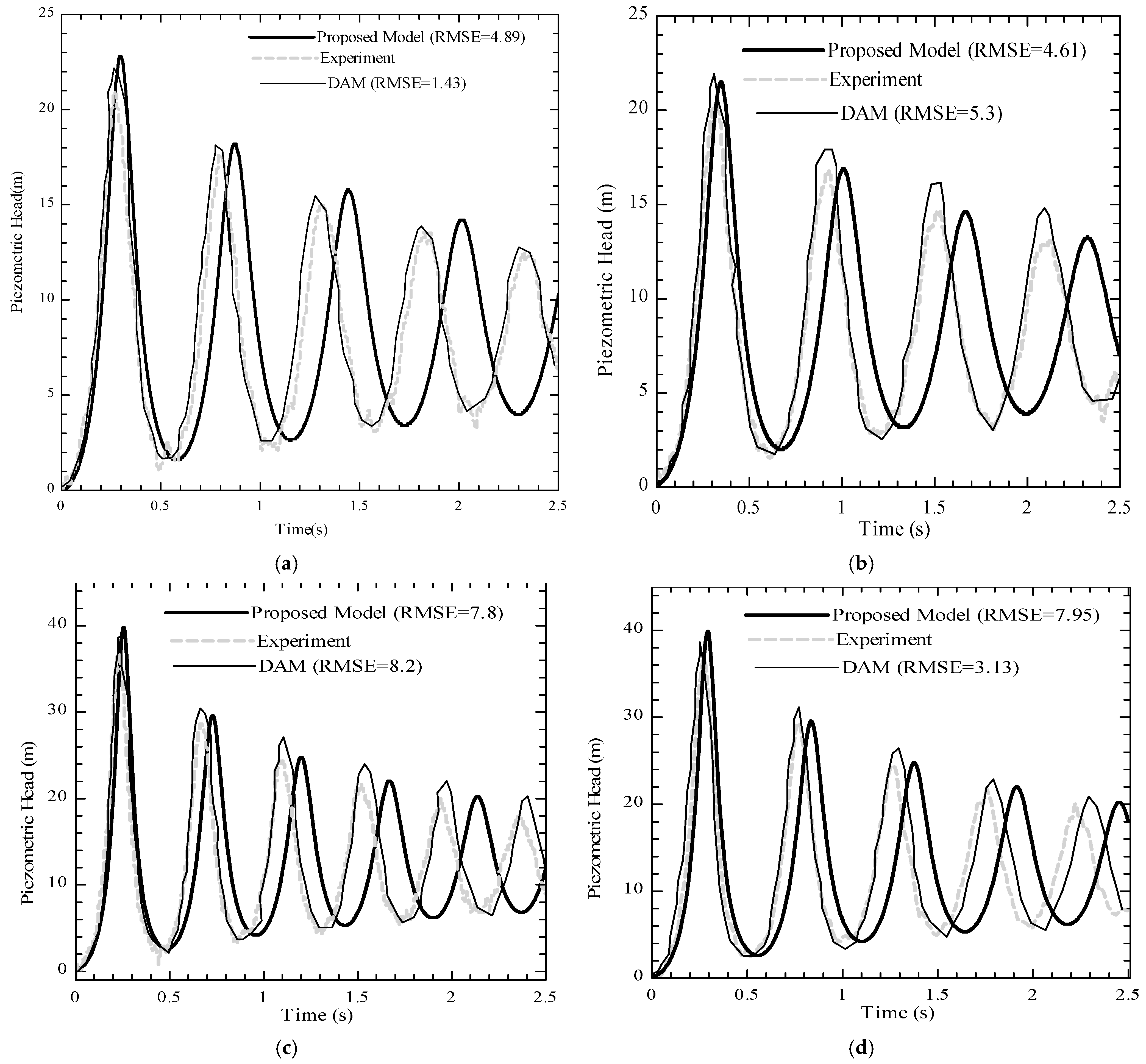
Further analysis in Figure 3 demonstrates that both models accurately estimate peak pressures during the first transient cycle. However, the proposed elastic model provides a more detailed representation of transient behavior under varying air–water interaction conditions. Since peak pressure in the first cycle is a key design factor, the model’s ability to capture it with high precision reinforces its relevance for engineering applications. Comparisons with the DAM in Figure 4 further confirm this, as both models exhibit high accuracy in estimating the initial peak—an essential aspect in pipeline design and pressure control. This observation is further supported by the quantitative results presented in

Table 2. Quantitative error metrics between model predictions and experimental data.

Case No.	Experimental Peak Pressure (m)	Proposed Model Peak Pressure (m)	RSME
1	21.64	21	1.06
2	29.06	28.2	2.38
3	46.82	46.1	4.93
4	20.79	22.8	4.89
5	21.5	20.24	4.61
6	39.8	36.63	7.8
7	36.63	39.9	7.95

, where the root mean square error (RMSE) values, ranging from 1.06 to 7.95. As shown in Table 2, the difference between the predicted and experimental first-cycle peak pressures is small across both experimental cases, highlighting the model’s strong agreement in capturing the most critical pressure response in transient conditions. While the agreement in the first transient cycle is strong, the model tends to slightly overestimate pressure amplitudes in subsequent cycles. This overestimation can be attributed to the assumption of a constant friction factor, whereas in reality, transient friction effects vary over time [27]. Duan et al. [25] demonstrated that unsteady friction significantly affects laboratory-scale experiments, especially in small-diameter systems. However, in real-world large-scale pipelines, as considered in this study, unsteady friction effects are less pronounced. Another potential source of discrepancy is the uniform air model (UAM) assumption. Feng et al. [8] found that when the ${\displaystyle \frac{L}{D}}$ ratio exceeds 2000, the UAM and the DAM produce similar results. Given that real-world pipelines typically have large ${\displaystyle \frac{L}{D}}$ ratios, assuming uniform air distribution can be considered a reasonable approximation. Additionally, neglecting heat transfer effects in numerical models can introduce deviations beyond the first transient cycle, as complex thermodynamic interactions occur within the air pocket during compression and expansion [31]. Future improvements in transient modeling should incorporate these effects to enhance predictive accuracy across diverse operating conditions.

As previously discussed, the highest transient pressure occurs during the first cycle, making its accurate prediction essential for pipeline design. Since one-dimensional models exhibit high accuracy in peak pressure estimation, they remain a reliable tool for transient flow analysis.

The length and diameter of experimental pipelines typically differ from those of real-world pipeline systems due to spatial and budgetary constraints in laboratory design. However, this study focuses on large-scale operational pipelines and proposes an optimal filling strategy for partially drained systems.

4. Numerical Results and Discussion

Numerical simulations are performed on a hypothetical pipeline (Figure 5), isolated from a larger system for maintenance. While hypothetical, this setup is designed to be broadly applicable to real-world pipeline operations. Most experimental studies focus on short, horizontal pipelines with upstream reservoirs and dead-end boundaries, limiting their relevance to large-scale, undulating systems. In this study, a long, undulating pipeline is considered, featuring an upstream reservoir at a constant elevation of 1100 m and a water level of 5 m. In this context, “large-scale” refers to pipelines with a length exceeding 10 km and a diameter above 0.8 m, which are commonly used in municipal and industrial water transmission systems.

The system consists of 13 pipes in series with a total length of 15,900 m, an internal diameter of 0.9 m, an acoustic wave speed of 1000 m/s, and a Darcy–Weisbach friction factor of 0.018. The last 1600 m of the pipeline is drained and isolated using a control valve, with a bypass system and air valve regulating air release during filling.

The control valve opening time plays a critical role in mitigating negative pressures during filling. As the control valve gradually opens, pressure waves propagate upstream, reflecting back as positive waves, reducing the intensity of negative pressures at the valve location. To prevent severe negative pressures, technical recommendations suggest that the valve opening time should be at least $2L/a$, allowing reflected waves to reach the valve before it fully opens. Given the 14,300 m water column and a wave speed of 1000 m/s, a 30 s valve opening duration is adopted, ensuring wave reflection reaches the valve before full opening. This duration balances pressure control with manual operational feasibility. Extending this time beyond 30 s is not feasible due to practical constraints.

To systematically assess the transient response of the system, ten different cases are analyzed, each varying in bypass diameter ($D_B$) and air valve nozzle diameter ($D_o$), as presented in

Table 3. Characteristic of cases for transient analysis.

Case No.	${\mathit{D}}_{\mathit{B}}\left(\mathbf{m}\right)$	${\mathit{D}}_{\mathit{o}}\left(\mathbf{m}\mathbf{m}\right)$
1	-	150
2	-	50
3	-	15
4	0.3	150
5	0.3	50
6	0.3	15
7	0.1	150
8	0.1	50
9	0.1	30
10	0.1	15

.

4.1. Air Expulsion Mechanism and Pressure Surge Formation

The pipeline filling process follows a two-stage air expulsion mechanism, where interactions between the trapped air pocket and the advancing water column drive transient pressure fluctuations.

• Stage a: Compression and Expansion of Trapped Air

Before complete air expulsion, the trapped air pocket compresses and expands, influencing transient pressure dynamics. A gradual air release cushions the advancing water column, dampening pressure surges, whereas rapid air expulsion accelerates water flow, increasing the potential for intense pressure fluctuations.

• Stage b: Water Hammer and Pressure Wave Propagation

Once the air pocket is fully expelled, the high-speed water column abruptly decelerates at the pipeline’s end, triggering a water hammer effect. This results in a sudden pressure surge, which propagates upstream as negative pressure reflections.

The severity of these pressure surges depends on air valve nozzle size and bypass line diameter, both of which regulate air release rates and control water column velocity. To accurately evaluate transient pressures during filling, this study investigates the effects of air valve nozzle size and bypass line diameter through numerical simulations, assessing their role in mitigating pressure surges at each stage.

4.2. Effect of Air Valve Nozzle Size on Transient Pressures

The air valve nozzle size plays a critical role in transient pressure control. A larger nozzle accelerates air expulsion, limiting compression–expansion cycles in Stage a. However, this rapid air release increases water column velocity, intensifying water hammer effects in Stage b. Figure 6b shows that for a 150 mm nozzle, the air pocket is fully expelled within 411 s, leading to an accelerated water column. Since air has a lower density than water, it escapes rapidly upon reaching the nozzle, intensifying water hammer effects [29]. In this scenario, air is quickly expelled from the system without experiencing significant compression–expansion cycles in Stage a. However, once the last air pocket exits, the high-speed water column impacts the pipe end, causing sudden deceleration and generating a severe water hammer effect. This overpressure propagates upstream, reflecting as negative pressure surges and amplifying transient oscillations throughout the system. Conversely, reducing the nozzle size restricts air release, prolonging air retention and increasing localized pressure before expulsion. The entrapped air pocket acts as a cushion, gradually absorbing transient pressures through repeated compression–expansion cycles. As shown in Figure 7a, higher air pocket pressure reduces the kinetic energy of the water column, thereby mitigating water hammer surges in Stage b. However, before the air pocket exits in Stage a, excessive air compression can still generate high transient pressures, which propagate upstream as negative reflections, leading to significant pressure differentials across the system.

To quantify transient responses under varying air release conditions, this study evaluates key hydraulic parameters including air pocket exit time ($T_{ex}$), pressure increase rate ($PIR$), pressure reduction rate ($PRR$), and water hammer pressure ($∆H$) in both stages of the filling process—indicated with indices 1 and 2—as defined in Equations (20) and (21) and

Table 4. Hydraulic parameters without considering the bypass line in cases 1 to 3.

Case No.	${\mathit{T}}_{\mathit{e}\mathit{x}}\left(\mathbf{s}\right)$	${\mathit{P}\mathit{I}\mathit{R}}_1$ (%)	${\mathit{P}\mathit{R}\mathit{R}}_1$ (%)	$∆{\mathit{H}}_1\left(\mathbf{m}\right)$	${\mathit{P}\mathit{I}\mathit{R}}_2$ (%)	${\mathit{P}\mathit{R}\mathit{R}}_2$ (%)	$∆{\mathit{H}}_2\left(\mathbf{m}\right)$
1	411.08	92.52	0.88	229.1	244.68	33.48	528
2	568.05	165.04	0.96	410.2	122.56	83.96	96.5
3	2167.51	171.6	0.96	426.6	103.36	100.64	6.8

. Table 4 presents these results for cases 1–3, where no bypass line is implemented. The findings indicate that while reducing the air valve nozzle diameter has minimal effect on negative pressure mitigation, it significantly lowers peak overpressures, reducing overall water hammer severity. However, despite this reduction in Stage b, peak pressures in Stage a remain considerably high due to excessive air compression before release.

$$PIR={\displaystyle \frac{H_{Max}-{\left(Elevation\right)}_{Bypass}}{H_{Static}}}$$

(20)

$$PRR={\displaystyle \frac{H_{Min}-{\left(Elevation\right)}_{Bypass}}{H_{Static}}}$$

(21)

Figure 6 and Figure 7 further demonstrate that reducing the nozzle diameter slows the water column after air expulsion, preventing a sharp pressure rise. While prolonged air retention slightly increases the total filling time, Table 4 confirms that in all tested cases, the air pocket is fully expelled, supporting the feasibility of this approach. The use of smaller nozzles aligns with AWWA recommendations, as it prevents sudden, explosive air release. However, to effectively control both overpressures and negative pressures, a bypass system should be incorporated to provide balanced pressure regulation throughout the pipeline.

4.3. Combined Effect of Bypass Line and Air Valve Nozzle on Pressure Regulation

Although reducing the air valve nozzle size helps mitigate Stage b pressure surges, significant pressure differentials still develop along the pipeline due to excessive air compression before expulsion. This occurs because a smaller nozzle restricts air outflow, leading to pressure rise and large variations before the air pocket is fully expelled. To further regulate transient pressures, an additional scenario is examined where a bypass line is integrated alongside air valve optimization to allow for better control of the valve diameter. A bypass line with a smaller diameter than the main pipeline is used to reduce water column velocity, thereby limiting its impact on the downstream boundary. This approach not only mitigates overpressures but also reduces pressure wave reflections. As shown in Figure 8, decreasing the bypass diameter reduces positive pressures at the downstream end, thereby minimizing their reflection back toward the reservoir. This dampening effect lowers the overall pressure differential between maximum and minimum system pressures, significantly attenuating water hammer surges. Additionally, as seen in Figure 8, incorporating a bypass line reduces water column velocity from approximately 4.4 m/s in a system without a bypass to about 0.54 m/s when a bypass with a 0.1 m diameter is used. Based on Joukowski’s formulation, reducing water column velocity directly lowers pressure differentials, effectively reducing water hammer intensity.

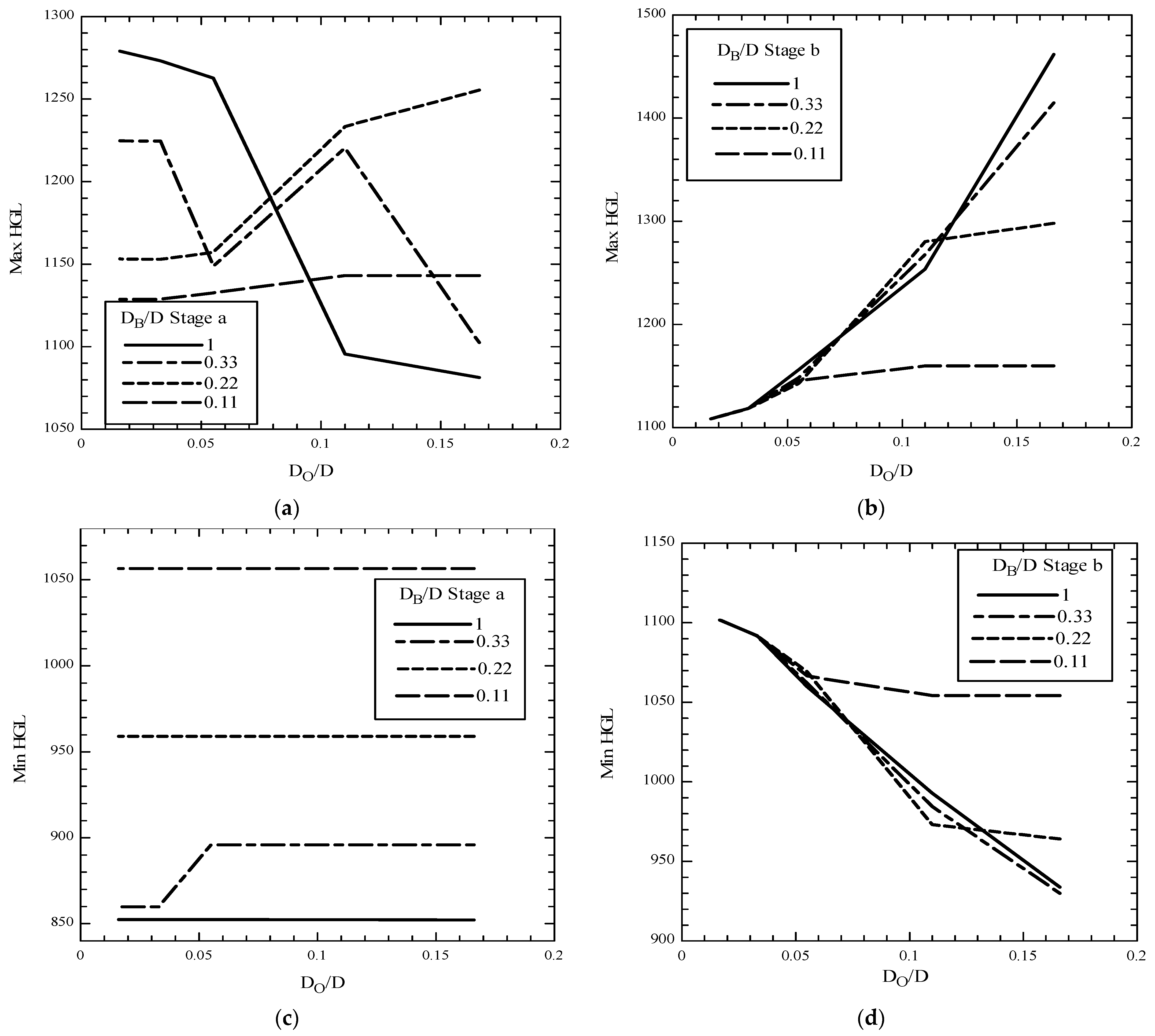
To systematically compare different cases, the bypass diameter ($D_B$) and air valve nozzle diameter ($D_o$) were normalized using the main pipeline diameter ($D$), yielding the dimensionless parameters ${\displaystyle \frac{D_B}{D}}$ and ${\displaystyle \frac{D_o}{D}}$. As illustrated in Figure 9, the maximum and minimum piezometric heads are analyzed based on these parameters. The findings indicate that decreasing ${\displaystyle \frac{D_o}{D}}$ enhances the damping effect of the trapped air, reducing overpressures after air expulsion. However, excessively small air valve nozzles prolong air retention time, amplifying transient pressures in the early stages of filling. Similarly, decreasing ${\displaystyle \frac{D_B}{D}}$ reduces the velocity of the advancing water column, thereby reducing both maximum overpressures and negative pressure reflections near the upstream reservoir.

A quantitative comparison of these effects is provided in

Table 5. Hydraulic parameters for cases 4 to 10.

Case No.	${\mathit{T}}_{\mathit{e}\mathit{x}}\left(\mathbf{s}\right)$	${\mathit{P}\mathit{I}\mathit{R}}_1$ (%)	${\mathit{P}\mathit{R}\mathit{R}}_1$ (%)	$∆{\mathit{H}}_1\left(\mathbf{m}\right)$	${\mathit{P}\mathit{I}\mathit{R}}_2$ (%)	${\mathit{P}\mathit{R}\mathit{R}}_2$ (%)	$∆{\mathit{H}}_2\left(\mathbf{m}\right)$
4	556.045	101	18.36	518.9	225.92	31.96	484.9
5	660.52	149.92	18.36	328.9	119.48	84.8	86.7
6	2264.632	149.88	18.36	328.8	103.36	100.64	6.8
7	2976.299	117.24	82.64	86.5	123.92	81.64	105.7
8	3012.334	113.04	82.64	76	118.32	86.6	79.3
9	3202.519	111.48	82.64	72.1	107.44	96.68	26.9
10	4447.075	111.48	82.64	72.1	103.36	100.64	6.8

, demonstrating that combining an optimized bypass line with a reduced air valve nozzle size significantly improves transient pressure regulation. A comparison of cases 4–10 reveals that when a properly sized bypass is implemented, both overpressures and negative pressures are substantially reduced. However, selecting an appropriate bypass diameter is crucial to balancing pressure mitigation with practical implementation constraints. While a smaller bypass diameter slightly increases overall filling time, this delay is negligible compared to the significant reduction in risks associated with entrapped air pockets.

4.4. Evaluating AWWA Filling Recommendations

The AWWA recommends two primary strategies to minimize the risks associated with trapped air pockets:

• Maintaining a slow filling velocity of 0.3 m/s;
• Using properly sized air valves to facilitate gradual air release under high pressures.

However, implementing a strictly controlled 0.3 m/s filling velocity is often impractical due to human error and limitations in precise flow control mechanisms. As demonstrated in previous sections, incorporating a properly sized bypass effectively reduces water column velocity. However, even with a 0.1 m bypass diameter, the calculated filling velocity remains 0.54 m/s, exceeding the AWWA guideline. To meet the recommended velocity, the bypass diameter would need to be reduced further to 0.08 m, which introduces operational challenges.

As the simulation results demonstrate, utilizing a bypass pipe with a diameter of 0.1 m effectively eliminates all negative pressures along the pipeline, maintains maximum pressures within safe thresholds, and ensures the complete expulsion of entrapped air pockets. Therefore, reducing the bypass diameter further—such as to 0.08 m, though not explicitly modeled in this study—would extend the total filling time to approximately 5914.24 s and introduce additional implementation challenges due to the reduced cross-sectional flow area. While this scenario technically complies with the AWWA’s recommended filling velocity, it is not considered necessary from an engineering perspective, given that the 0.1 m bypass already achieves full air removal and significantly mitigates pressure surges. Hence, further reduction in bypass diameter offers limited additional benefit while imposing avoidable operational constraints.

5. Conclusions

Optimizing the pipeline filling process requires a careful balance between minimizing negative pressures, mitigating water hammer surges, and ensuring operational feasibility. Given the cost and complexity of physical testing, this study employs a high-precision one-dimensional numerical model to simulate a long, undulating pipeline, ensuring its applicability to real-world systems. The model’s accuracy is validated through comparisons with experimental data from two setups—one featuring an air valve and the other a dead-end pipeline. Additionally, its reliability in predicting transient flow behavior is assessed against two numerical approaches—the Rigid Column Model and the Discrete Air Model—demonstrating its effectiveness in capturing key pressure dynamics.

This study analyzes the influence of air valve nozzle sizes and bypass pipe diameters on transient pressures. Numerical trials based on AWWA recommendations indicate that larger air valve nozzles allow for rapid air expulsion without inducing a significant pressure rise in Stage a. However, once air is fully released, the high-velocity water column impacts the pipeline’s end, triggering severe water hammer pressures in Stage b. Conversely, reducing the nozzle diameter prolongs air retention, introducing compression–expansion cycles that help moderate surges after air expulsion. While this approach effectively reduces sudden pressure spikes, it also results in elevated peak pressures in the early filling stage, generating negative pressure waves propagating upstream.

To address these challenges, an additional scenario incorporates a bypass line. The results indicate that introducing a bypass with a smaller diameter than the main pipeline effectively reduces water column velocity, thereby lowering transient pressures throughout the system. This approach significantly dampens overpressures and mitigates negative pressure reflections near the upstream reservoir. However, while reducing the bypass diameter effectively controls transient pressures, excessive reduction extends the filling time, posing practical constraints for implementation.

Overall, this study establishes a reliable numerical foundation for optimizing pipeline filling strategies. The findings underscore the importance of balancing transient pressure control with operational feasibility, ensuring that proposed solutions remain both effective and applicable to real-world pipeline systems. Building on the validated one-dimensional model presented here, future efforts could explore the development of a coupled modeling framework, in which the main pipeline is represented through a 1D elastic model, while the downstream unfilled section—where air–water interactions dominate—is resolved using a localized 3D approach. This type of hybrid modeling would allow for a more detailed treatment of transient air pocket behavior, including non-uniform air distribution, complex interface dynamics, and thermodynamic effects such as heat transfer between compressed air, water, and pipe walls.