


Combining Crop and Water Decisions to Manage Groundwater Overdraft over Decadal and Longer Timescales


Abstract
1. Introduction
2. Materials and Methods
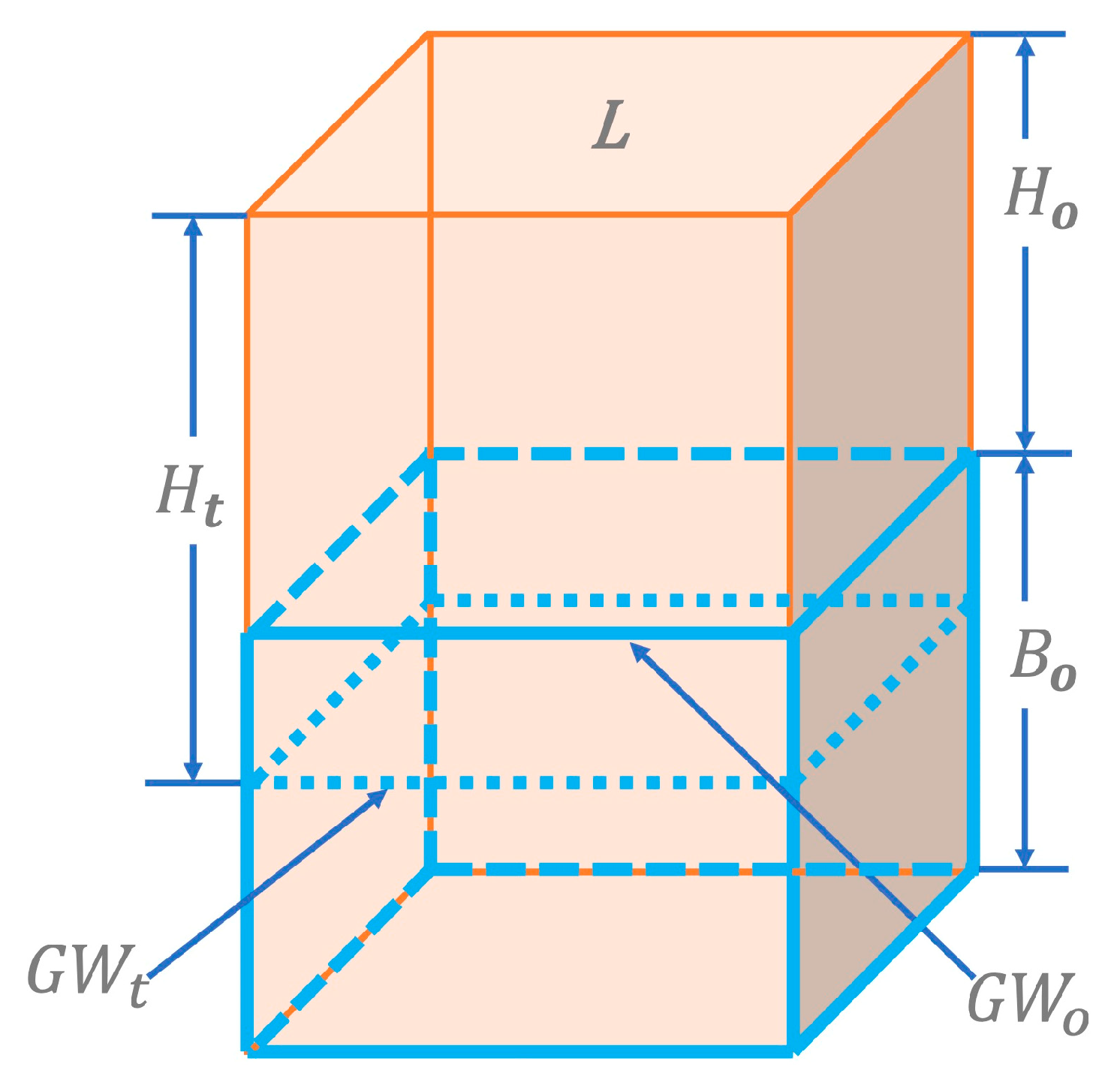
2.1. Inner Model Formulation
2.2. Outer Model Formulation
2.3. Model Assumptions and Limitations
2.4. Case Example
3. Results
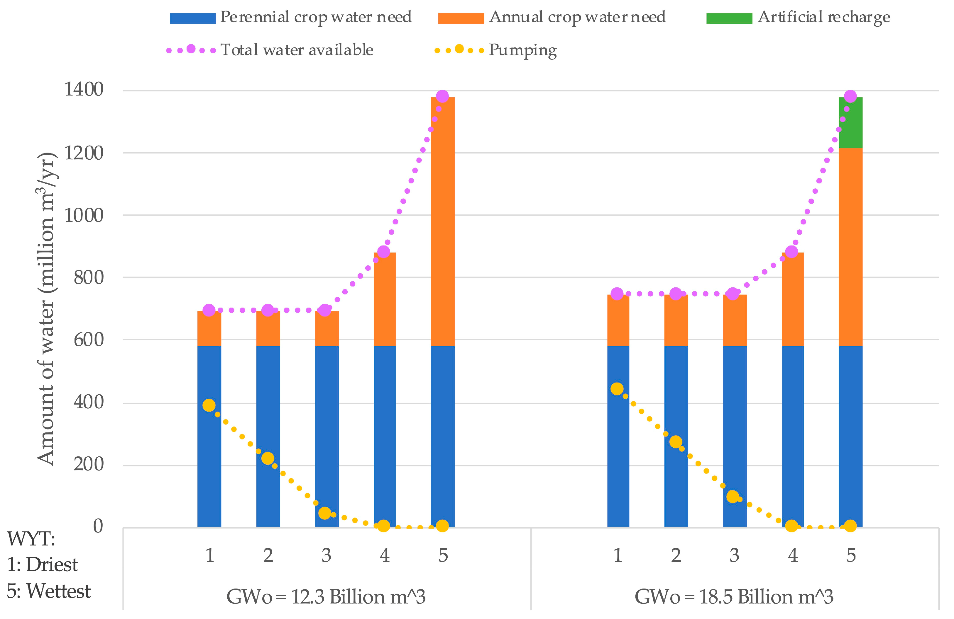
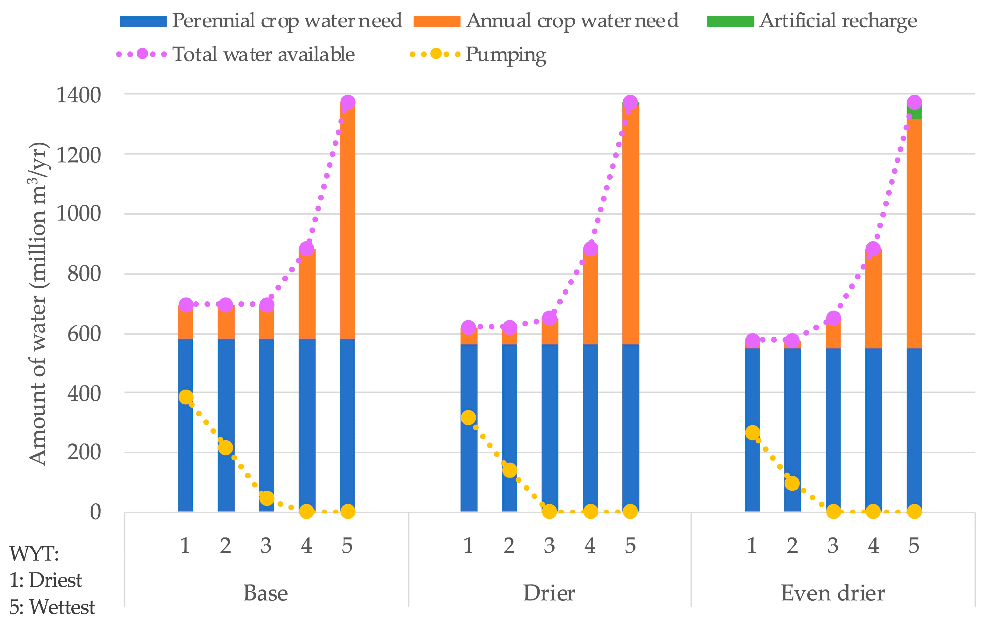
3.1. Conjunctive Use and Cropping for Within-decade Timescales
3.2. Groundwater Management and Cropping for Long-Term Timescales
3.3. Sensitivity Analyses
3.3.1. Different Discount Rates
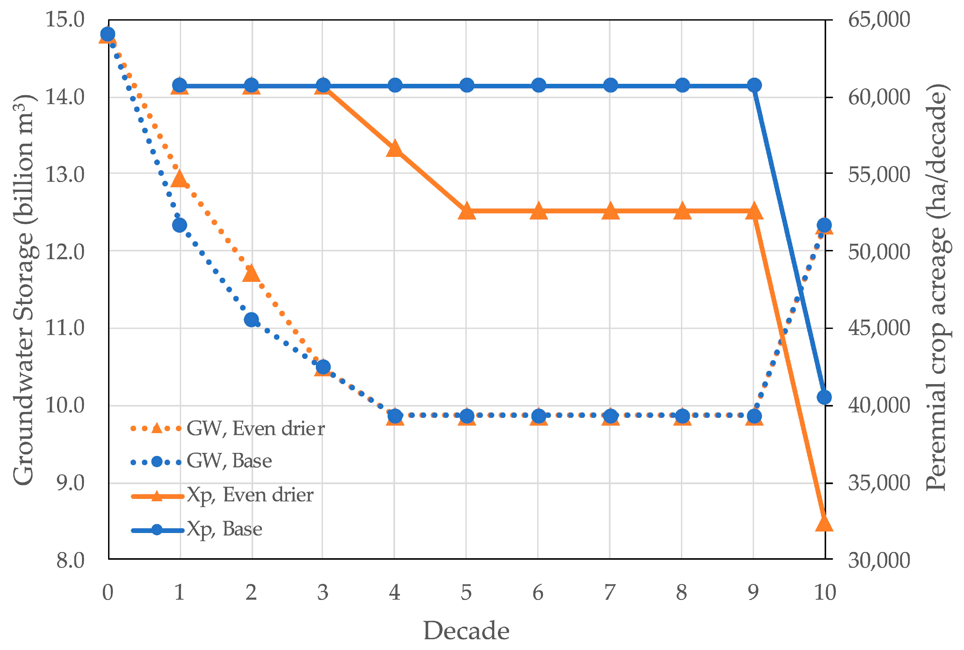
3.3.2. Climate Effects
4. Conclusions
Author Contributions
Funding
Data Availability Statement
Acknowledgments
Conflicts of Interest
Appendix A

| Parameter (Unit) | Perennial Crop (Similar to Almonds) | Annual Crop (Similar to Alfalfa) | |
|---|---|---|---|
| Base year observations | (ha) | 132,874 | 67,724 |
| (kg/ha) | 2242 | 17,934 | |
| ($/kg) | 4.66 | 0.173 | |
| (m/ha) | 3.07 | 3.65 | |
| Land cost ($/ha) | 2006 | 783 | |
| Other supply cost ($/ha) | 4146 | 1344 | |
| Labor cost ($/ha) | 786 | 52 | |
| Total cost ($/ha) | 6939 | 2179 | |
| PMP cost function | ($/ha) | 3713.62 | 1571.37 |
| ($/ha2) | 0.0485 | 0.0180 |
References
- Reilly, T.E.; Dennehy, K.F.; Alley, W.M.; Cunningham, W.L. Ground-Water Availability in the United States; Geological Survey (US): Reston, VA, USA, 2008; ISBN 1-4113-2183-9.
- Faunt, C. Groundwater Availability of the Central Valley Aquifer. U.S. Geol. Surv. Prof. Pap. 2009, 1766, 225. [Google Scholar]
- Lund, J.; Medellin-Azuara, J.; Durand, J.; Stone, K. Lessons from California’s 2012–2016 Drought. J. Water Resour. Plann. Manag. 2018, 144, 04018067. [Google Scholar] [CrossRef]
- Escriva-Bou, A.; Hui, R.; Maples, S.; Medellín-Azuara, J.; Harter, T.; Lund, J.R. Planning for Groundwater Sustainability Accounting for Uncertainty and Costs: An Application to California’s Central Valley. J. Environ. Manag. 2020, 264, 110426. [Google Scholar] [CrossRef] [PubMed]
- Chen, X.; Hu, Q. Groundwater Influences on Soil Moisture and Surface Evaporation. J. Hydrol. 2004, 297, 285–300. [Google Scholar] [CrossRef]
- Pauloo, R.A.; Fogg, G.E.; Guo, Z.; Harter, T. Anthropogenic Basin Closure and Groundwater Salinization (ABCSAL). J. Hydrol. 2021, 593, 125787. [Google Scholar] [CrossRef]
- Yao, Y.; Lund, J.R.; Harter, T. Conjunctive Water Management for Agriculture with Groundwater Salinity. Water Resour. Res. 2022, 58, e2021WR031058. [Google Scholar] [CrossRef]
- Romero, E. Friant-Kern Canal Slows By 60 Percent, Subsidence To Blame. Available online: https://www.kvpr.org/environment/2017-08-03/friant-kern-canal-slows-by-60-percent-subsidence-to-blame (accessed on 22 April 2024).
- California Department of Water Resources California Aqueduct Subsidence Study. Available online: https://cawaterlibrary.net/wp-content/uploads/2017/11/Aqueduct_Subsidence_Study-FINAL-2017.pdf (accessed on 22 April 2024).
- Harou, J.J.; Lund, J.R. Ending Groundwater Overdraft in Hydrologic-Economic Systems. Hydrogeol. J. 2008, 16, 1039. [Google Scholar] [CrossRef]
- Dogan, M.S.; Buck, I.; Medellin-Azuara, J.; Lund, J.R. Statewide Effects of Ending Long-Term Groundwater Overdraft in California. J. Water Resour. Plan. Manag. 2019, 145, 04019035. [Google Scholar] [CrossRef]
- Alam, S.; Gebremichael, M.; Li, R.; Dozier, J.; Lettenmaier, D.P. Can Managed Aquifer Recharge Mitigate the Groundwater Overdraft in California’s Central Valley? Water Resour. Res. 2020, 56, e2020WR027244. [Google Scholar] [CrossRef]
- Buras, N. Conjunctive Operation of Dams and Aquifers. J. Hydraul. Div. 1963, 89, 111–131. [Google Scholar] [CrossRef]
- Burt, O.R. The Economics of Conjunctive Use of Ground and Surface Water. Hilg 1964, 36, 31–111. [Google Scholar] [CrossRef]
- Burt, O.R. Economic Control of Groundwater Reserves. Am. J. Agric. Econ. 1966, 48, 632–647. [Google Scholar] [CrossRef]
- Bredehoeft, J.D.; Young, R.A. Conjunctive Use of Groundwater and Surface Water for Irrigated Agriculture: Risk Aversion. Water Resour. Res. 1983, 19, 1111–1121. [Google Scholar] [CrossRef]
- Fredericks, J.W.; Labadie, J.W.; Altenhofen, J.M. Decision Support System for Conjunctive Stream-Aquifer Management. J. Water Resour. Plan. Manag. 1998, 124, 69–78. [Google Scholar] [CrossRef]
- Pulido-Velázquez, M.; Andreu, J.; Sahuquillo, A. Economic Optimization of Conjunctive Use of Surface Water and Groundwater at the Basin Scale. J. Water Resour. Plan. Manag. 2006, 132, 454–467. [Google Scholar] [CrossRef]
- Gorelick, S.M. A Review of Distributed Parameter Groundwater Management Modeling Methods. Water Resour. Res. 1983, 19, 305–319. [Google Scholar] [CrossRef]
- Bazargan-Lari, M.R.; Kerachian, R.; Mansoori, A. A Conflict-Resolution Model for the Conjunctive Use of Surface and Groundwater Resources That Considers Water-Quality Issues: A Case Study. Environ. Manag. 2009, 43, 470–482. [Google Scholar] [CrossRef]
- Tabari, M.M.R.; Soltani, J. Multi-Objective Optimal Model for Conjunctive Use Management Using SGAs and NSGA-II Models. Water Resour. Manag. 2013, 27, 37–53. [Google Scholar] [CrossRef]
- Naghdi, S.; Bozorg-Haddad, O.; Khorsandi, M.; Chu, X. Multi-Objective Optimization for Allocation of Surface Water and Groundwater Resources. Sci. Total Environ. 2021, 776, 146026. [Google Scholar] [CrossRef]
- Varela-Ortega, C.; Blanco-Gutiérrez, I.; Swartz, C.H.; Downing, T.E. Balancing Groundwater Conservation and Rural Livelihoods under Water and Climate Uncertainties: An Integrated Hydro-Economic Modeling Framework. Glob. Environ. Change 2011, 21, 604–619. [Google Scholar] [CrossRef]
- Rouhi Rad, M.; Haacker, E.M.K.; Sharda, V.; Nozari, S.; Xiang, Z.; Araya, A.; Uddameri, V.; Suter, J.F.; Gowda, P. MOD$$AT: A Hydro-Economic Modeling Framework for Aquifer Management in Irrigated Agricultural Regions. Agric. Water Manag. 2020, 238, 106194. [Google Scholar] [CrossRef]
- Ali, A.A.; Tran, D.Q.; Kovacs, K.F.; Dahlke, H.E. Hydro-economic Modeling of Managed Aquifer Recharge in the Lower Mississippi. J. Am. Water Resour. Assoc. 2023, 59, 1413–1434. [Google Scholar] [CrossRef]
- Marques, G.F.; Lund, J.R.; Howitt, R.E. Modeling Conjunctive Use Operations and Farm Decisions with Two-Stage Stochastic Quadratic Programming. J. Water Resour. Plan. Manag. 2010, 136, 386–394. [Google Scholar] [CrossRef]
- Gorelick, S.M.; Voss, C.I.; Gill, P.E.; Murray, W.; Saunders, M.A.; Wright, M.H. Aquifer Reclamation Design: The Use of Contaminant Transport Simulation Combined With Nonlinear Programing. Water Resour. Res. 1984, 20, 415–427. [Google Scholar] [CrossRef]
- Sedki, A.; Ouazar, D. Simulation-Optimization Modeling for Sustainable Groundwater Development: A Moroccan Coastal Aquifer Case Study. Water Resour. Manag. 2011, 25, 2855–2875. [Google Scholar] [CrossRef]
- Singh, A. Conjunctive Use of Water Resources for Sustainable Irrigated Agriculture. J. Hydrol. 2014, 519, 1688–1697. [Google Scholar] [CrossRef]
- Hazell, P.; Norton, R. Mathematical Programming for Economic Analysis in Agriculture; Macmillan Publishing Company: New York, NY, USA, 1986; ISBN 978-0-02-947930-8. [Google Scholar]
- Howitt, R.E. Positive Mathematical Programming. Am. J. Agric. Econ. 1995, 77, 329–342. [Google Scholar] [CrossRef]
- Yeh, W.W.-G. Reservoir Management and Operations Models: A State-of-the-Art Review. Water Resour. Res. 1985, 21, 1797–1818. [Google Scholar] [CrossRef]
- Shang, S.; Mao, X. Application of a Simulation Based Optimization Model for Winter Wheat Irrigation Scheduling in North China. Agric. Water Manag. 2006, 85, 314–322. [Google Scholar] [CrossRef]
- Kuwayama, Y.; Brozović, N. The Regulation of a Spatially Heterogeneous Externality: Tradable Groundwater Permits to Protect Streams. J. Environ. Econ. Manag. 2013, 66, 364–382. [Google Scholar] [CrossRef]
- Yakowitz, S. Dynamic Programming Applications in Water Resources. Water Resour. Res. 1982, 18, 673–696. [Google Scholar] [CrossRef]
- Philbrick, C.R.; Kitanidis, P.K. Optimal Conjunctive-Use Operations and Plans. Water Resour. Res. 1998, 34, 1307–1316. [Google Scholar] [CrossRef]
- Karamouz, M.; Kerachian, R.; Zahraie, B. Monthly Water Resources and Irrigation Planning: Case Study of Conjunctive Use of Surface and Groundwater Resources. J. Irrig. Drain. Eng. 2004, 130, 391–402. [Google Scholar] [CrossRef]
- Azaiez, M.N.; Hariga, M.; Al-Harkan, I. A Chance-Constrained Multi-Period Model for a Special Multi-Reservoir System. Comput. Oper. Res. 2005, 32, 1337–1351. [Google Scholar] [CrossRef]
- Yaron, D.; Dinar, A. Optimal Allocation of Farm Irrigation Water during Peak Seasons. Am. J. Agric. Econ. 1982, 64, 681–689. [Google Scholar] [CrossRef]
- Dudley, N.J.; Howell, D.T.; Musgrave, W.F. Optimal Intraseasonal Irrigation Water Allocation. Water Resour. Res. 1971, 7, 770–788. [Google Scholar] [CrossRef]
- Dudley, N.J.; Burt, O.R. Stochastic Reservoir Management and System Design for Irrigation. Water Resour. Res. 1973, 9, 507–522. [Google Scholar] [CrossRef]
- Gupta, R.K.; Chauhan, H.S. Stochastic Modeling of Irrigation Requirements. J. Irrig. Drain. Eng. 1986, 112, 65–76. [Google Scholar] [CrossRef]
- Davidsen, C.; Pereira-Cardenal, S.J.; Liu, S.; Mo, X.; Rosbjerg, D.; Bauer-Gottwein, P. Using Stochastic Dynamic Programming to Support Water Resources Management in the Ziya River Basin, China. J. Water Resour. Plan. Manag. 2015, 141, 04014086. [Google Scholar] [CrossRef]
- Soleimani, S.; Bozorg-Haddad, O.; Loáiciga, H.A. Reservoir Operation Rules with Uncertainties in Reservoir Inflow and Agricultural Demand Derived with Stochastic Dynamic Programming. J. Irrig. Drain. Eng. 2016, 142, 04016046. [Google Scholar] [CrossRef]
- Anvari, S.; Mousavi, S.J.; Morid, S. Stochastic Dynamic Programming-Based Approach for Optimal Irrigation Scheduling under Restricted Water Availability Conditions. Irrig. Drain. 2017, 66, 492–500. [Google Scholar] [CrossRef]
- Safavi, H.R.; Alijanian, M.A. Optimal Crop Planning and Conjunctive Use of Surface Water and Groundwater Resources Using Fuzzy Dynamic Programming. J. Irrig. Drain. Eng. 2011, 137, 383–397. [Google Scholar] [CrossRef]
- Franklin, B.; Schwabe, K.; Levers, L. Perennial Crop Dynamics May Affect Long-Run Groundwater Levels. Land 2021, 10, 971. [Google Scholar] [CrossRef]
- Zhu, T.; Marques, G.F.; Lund, J.R. Hydroeconomic Optimization of Integrated Water Management and Transfers under Stochastic Surface Water Supply. Water Resour. Res. 2015, 51, 3568–3587. [Google Scholar] [CrossRef]
- Yao, Y. Managing Groundwater for Agriculture, with Hydrologic Uncertainty and Salinity; University of California: Davis, CA, USA, 2021. [Google Scholar]
- Rao, N.H.; Sarma, P.B.S.; Chander, S. Optimal Multicrop Allocation of Seasonal and Intraseasonal Irrigation Water. Water Resour. Res. 1990, 26, 551–559. [Google Scholar] [CrossRef]
- Paul, S.; Panda, S.N.; Kumar, D.N. Optimal Irrigation Allocation: A Multilevel Approach. J. Irrig. Drain. Eng. 2000, 126, 149–156. [Google Scholar] [CrossRef]
- Ghahraman, B.; Sepaskhah, A.-R. Optimal Allocation of Water from a Single Purpose Reservoir to an Irrigation Project with Pre-Determined Multiple Cropping Patterns. Irrig. Sci. 2002, 21, 127–137. [Google Scholar] [CrossRef]
- CH2MHILL DRAFT Agricultural Economics Technical Appendix. Available online: https://web.archive.org/web/20170711215918/http://water.ca.gov/economics/downloads/Models/SWAP_TechAppendix_080612_Draft.pdf (accessed on 22 April 2024).


| Symbol | Parameter | Value (Unit) |
|---|---|---|
| T | Length of planning horizon | 10 (yr) |
| L | Total available area | 202,343 ha (500,000 acre) |
| Ho | Initial pump head | 60.96 m (200 ft) |
| Bo | Initial thickness of the aquifer | 60.96 m (200 ft) |
| sy | Aquifer specific yield | 0.1 |
| r | Constant discount rate for inner model | 3.5% |
| inip | Perennial crop initial establishment cost | $29,653/ha ($12,000/acre) |
| cland | Unit price of land for recharging | $741/ha ($300/acre) |
| cclass1 | Unit price of class 1 (firm contract) water | $0.034/m3 ($42/AF) |
| cclass2 | Unit price of class 2 (surplus) water | $0.024/m3 ($30/AF) |
| class1 | Amount of firm contract water | 617 million m3/yr (500 TAF/yr) |
| ce | Unit price of energy | $0.189/kWh |
| ηp | Pumping efficiency | 0.7 |
| cap | Capacity of land for recharging | 4.572 m/yr (15 ft/yr) |
| 1 − φ | Irrigation efficiency | 0.85 |
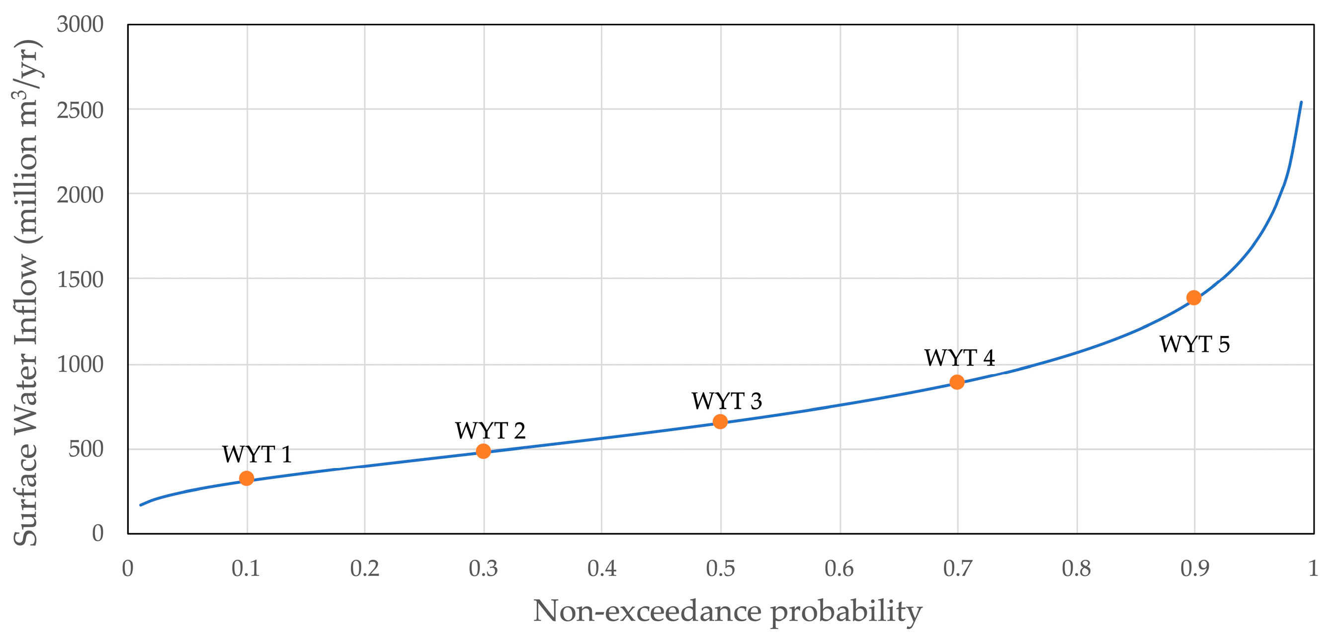
| WYT j | Percentile | swj (Million m3/yr) | pj |
|---|---|---|---|
| 1 (Dry) | 10th | 306 | 0.2 |
| 2 | 30th | 478 | 0.2 |
| 3 | Median | 649 | 0.2 |
| 4 | 70th | 883 | 0.2 |
| 5 (Wet) | 90th | 1376 | 0.2 |
| ∆GW (Billion m3) | Economic Values of Water ($/m3) | |||||
|---|---|---|---|---|---|---|
| Dry | Surface Water | Wet | Groundwater | |||
| WYT 1 | WYT 2 | WYT 3 | WYT 4 | WYT 5 | ||
| −1.23 | 0.14 | 0.14 | 0.14 | 0.14 | 0.078 | 0.031 |
| 0 | 0.17 | 0.17 | 0.17 | 0.15 | 0.079 | 0.049 |
| 1.23 | 0.23 | 0.23 | 0.18 | 0.15 | 0.13 | 0.079 |
| 2.47 | 0.28 | 0.28 | 0.182 | 0.182 | 0.182 | 0.105 |
| Xa (ha/yr) | Xr (ha/yr) | Wp (Million m3/yr) | |||||
|---|---|---|---|---|---|---|---|
| GWt − 1 (Billion m3) | 12.3 | 18.5 | 12.3 | 18.5 | 12.3 | 18.5 | |
| WYT j | 1 (Dry) | 7537 | 11,140 | 0 | 0 | 389 | 442 |
| 2 | 7537 | 11,140 | 0 | 0 | 217 | 271 | |
| 3 | 7537 | 11,140 | 0 | 0 | 46 | 99 | |
| 4 | 20,276 | 20,276 | 0 | 0 | 0 | 0 | |
| 5 (Wet) | 53,692 | 42,883 | 0 | 3488 | 0 | 0 | |
| WYT j | Climates | ||
|---|---|---|---|
| Even Drier | Drier | Base | |
| 1 (Dry) | 0.3 | 0.25 | 0.2 |
| 2 | 0.3 | 0.25 | 0.2 |
| 3 | 0.2 | 0.2 | 0.2 |
| 4 | 0.1 | 0.2 | 0.2 |
| 5 (Wet) | 0.1 | 0.1 | 0.2 |
| Expected incoming surface water (million m3/yr) | 591 (−20%) | 640 (−13%) | 739 |
| Climates | Even Drier | Drier | Base | ||||||
|---|---|---|---|---|---|---|---|---|---|
| Xp (ha/Decade) | 44,158 | 45,123 | 47,058 | ||||||
| Second Stage Decisions | Xa | Xr | Wp | Xa | Xr | Wp | Xa | Wp | |
| (ha/yr) | (ha/yr) | (m3/yr) | (ha/yr) | (ha/yr) | (m3/yr) | (ha/yr) | (m3/yr) | ||
| WYT j | 1 (Dry) | 1899 | 0 | 269 × 106 | 4142 | 0 | 314 × 106 | 7537 | 389 × 106 |
| 2 | 1899 | 0 | 98 × 106 | 4142 | 0 | 143 × 106 | 7537 | 217 × 106 | |
| 3 | 6882 | 0 | 0 | 6071 | 0 | 0 | 7537 | 46 × 106 | |
| 4 | 22,715 | 0 | 0 | 21,903 | 0 | 0 | 20,276 | 0 | |
| 5 (Wet) | 52,064 | 1312 | 0 | 54,307 | 327 | 0 | 53,692 | 0 | |
| Climates | Economic Values of Water ($/m3) | |||||
|---|---|---|---|---|---|---|
| Dry | Surface Water | Wet | Groundwater | |||
| WYT 1 | WYT 2 | WYT 3 | WYT 4 | WYT 5 | ||
| Base | 0.17 | 0.17 | 0.17 | 0.147 | 0.079 | 0.049 |
| Drier | 0.23 | 0.23 | 0.177 | 0.145 | 0.040 | 0.053 |
| Even drier | 0.28 | 0.28 | 0.184 | 0.072 | 0.042 | 0.056 |
| Initial Groundwater Storage GWo (Billion m3) | Climate Change | |
|---|---|---|
| Even Drier to Drier | Drier to Base | |
| 9.87 | 0.36 | 0.28 |
| 11.1 | 0.34 | 0.24 |
| 12.3 | 0.30 | 0.22 |
| 13.6 | 0.28 | 0.21 |
| 14.8 | 0.27 | 0.20 |
| Groundwater Storage Change (Billion m3) | Climates | ||
|---|---|---|---|
| Even Drier | Drier | Base | |
| 9.87 to 11.1 | 0.095 | 0.087 | 0.057 |
| 11.1 to 12.3 | 0.075 | 0.060 | 0.046 |
| 12.3 to 13.6 | 0.062 | 0.051 | 0.044 |
| 13.6 to 14.8 | 0.057 | 0.051 | 0.043 |
Disclaimer/Publisher’s Note: The statements, opinions and data contained in all publications are solely those of the individual author(s) and contributor(s) and not of MDPI and/or the editor(s). MDPI and/or the editor(s) disclaim responsibility for any injury to people or property resulting from any ideas, methods, instructions or products referred to in the content. |
© 2024 by the authors. Licensee MDPI, Basel, Switzerland. This article is an open access article distributed under the terms and conditions of the Creative Commons Attribution (CC BY) license (https://creativecommons.org/licenses/by/4.0/).
Share and Cite
Yao, Y.; Lund, J.R.; Medellín-Azuara, J. Combining Crop and Water Decisions to Manage Groundwater Overdraft over Decadal and Longer Timescales. Water 2024, 16, 1223. https://doi.org/10.3390/w16091223
Yao Y, Lund JR, Medellín-Azuara J. Combining Crop and Water Decisions to Manage Groundwater Overdraft over Decadal and Longer Timescales. Water. 2024; 16(9):1223. https://doi.org/10.3390/w16091223
Chicago/Turabian StyleYao, Yiqing, Jay R. Lund, and Josué Medellín-Azuara. 2024. "Combining Crop and Water Decisions to Manage Groundwater Overdraft over Decadal and Longer Timescales" Water 16, no. 9: 1223. https://doi.org/10.3390/w16091223
APA StyleYao, Y., Lund, J. R., & Medellín-Azuara, J. (2024). Combining Crop and Water Decisions to Manage Groundwater Overdraft over Decadal and Longer Timescales. Water, 16(9), 1223. https://doi.org/10.3390/w16091223