Abstract
Climate change causes the river basin water cycle disorders, and rainfall characteristics frequently result in flood disasters. This study aims to simulate and assess the response behavior of basin floods under the influence of rainfall characteristics and land use changes in the Hulu River basin using a 2D hydrological and hydraulic GAST (GPU Accelerated Surface Water Flow and Transport Model). The peak flow rate and water depth during floods were examined by simulating the evolution process of basin floods and related hydraulic elements under the independent effects of various rainfall characteristics or land use and further simulating the response results of basin floods under the combined effects of rainfall characteristics and land use. The seven scenarios were set to quantify the degree of influence that land use and rainfall characteristics have on the basin flood process based on examining changes in land use and rainfall characteristics in the research area. The results from different rainfall characteristics scenarios depicted that as the rainfall return period is shorter, the peak flow rate is higher, and the peak flow rate is lower as the return period is prolonged. Under different rainfall characteristics, the peak flow rate in scenario R8 is 41.30%, 40.00%, and 34.51% higher than the uniform distribution of rainfall, while water depth is decreased by 0.55%, increased by 4.96% and 2.92% as compared to the uniform distribution of rainfall. While under different land use scenarios, it is observed that the change in land use has increased 2.7% in cultivated land and 1.1% in woodland. In addition, the interactive effect of different rainfall characteristics and land use it can be seen that the scenario with the greatest reduction in flood risk due to rainfall characteristics and land use is RL2-4, representing a 12.55% decrease in peak flow and a 37.69% decrease in peak water depth. In this scenario, the rainfall is heavier in the southeast and northwest regions and lighter in the northeast and southwest regions. The land use type is characterized by reforestation and the return of cultivated land to forests. The changes in rainfall distribution and the increase in grassland contribute to the decrease in flood threat. Future research in the erodible parts of the Hulu River basin, planning for water resources, and soil and water conservation can all benefit from the study’s conclusions.
1. Introduction
Life requires access to water resources and has enormous socioeconomic significance in various industries, including agriculture, manufacturing, trade, food production, and hydropower generation [1,2]. It is well acknowledged that human activity and climate change significantly impact the hydrological cycle and the spatiotemporal patterns of rainfall [3]. According to [4], streamflow in most rivers has been steadily declining over the past few decades, leading to serious water shortages and ecological and environmental instability. Climate change and human activity typically work together to impact river streamflow changes [5]. One of the most dependable ways to assess changes in water resources is to combine climate prediction data from general circulation models (GCMs) with hydrological models [6]. Many hydrological modeling studies have been conducted since the end of the 1950s to assess the effects of changes in land use on the rainfall–runoff regime and the magnitude and frequency of floods [7]. Study [8] examines how changes in upstream land use affect downstream flood patterns using the HEC-1 model. Study [9] indicates that changes in land use significantly impact the magnitude of flood peaks and runoff volume. The authors of [10] use the hydrological SWAT model to evaluate how changes in land use affect a mesoscale catchment’s annual water balance and temporal runoff dynamics. The authors of [11] analyzed the Impact of Land-Use Changes on Flood Exposure. The impact of urban sprawl on eco-environmental quality in China, using the Spatial Durbin model and panel data from 2003 to 2018, highlighting significant regional variations and the predominant influence of land use sprawl [12]. Various scholars have used multiple GCMs to evaluate how climate change affects streamflow, thus confirming its role. For example, in the Kashafrud River Basin (KRB) in Iran [13], streamflow has shown increasing trends under various scenarios. In the Kelantan River Basin, precipitation, temperature and streamflow have been predicted to increase from 2015 to 2044 and from 2045 to 2074 [14]. Currently, the Coupled Model Inter-Comparison Project, which is conducting global climate research, has reached its sixth phase, providing more comprehensive evaluations of future global climate [15]. A combined weighting approach and the super-efficiency Slack-Based Measure (SBM) model to assess urban–rural integration and land-use efficiency in China, revealing a low overall level and a trend towards improved coordination over the decade from 2010 to 2019 [16].
In China, including in the Yellow River Basin [17], Biliu River Basin [18], and Luan River Basin [19], future streamflow is expected to show downward trends at varying degrees. The two main elements influencing flood formation are the climate and the state of the underlying surface. The impact of precipitation and intensity on the production of runoff is a major factor in how climate change will affect the runoff process. Numerous studies have shown that precipitation impacts how runoff changes in a watershed. A rise in the amount of rainfall causes an increase in runoff if the underlying surface remains the same [20,21]. However, the alteration of confluence and runoff generation circumstances brought on by variations within the subsurface conditions are the primary variables influencing the environmental changes that lead to flood formation. Human activity impacts these changes, including clearing forest vegetation, building hydraulic infrastructure on rivers, extensive irrigation and drainage, water and soil conservation measures, modifications to land-use patterns, and urbanization and industrialization [22,23]. The critical issue of optimal city size to enhance Resource and Environment Intensity (REI) in China, analyzing the spatial–temporal impact of city size on REI within the Yangtze River Economic Belt through spatial models and panel data from 2004 to 2019. The literature review likely examines previous findings on urban expansion, resource efficiency, and spatial governance, setting the stage for this study’s unique contribution to understanding the nuanced relationship between city size and REI [24].
As a result of agricultural practices, humans have gradually altered the earth’s surface in important ways. More than 50% of the earth’s surface has recently changed, with estimates placing agriculture on nearly one-third of the planet’s surface [25]. The conversion of the naturally occurring agricultural land ratio to other land is still in progress [26]. Land use managers and decision-makers can better understand the connections between human and natural activity by looking at the patterns in change detection, which has drawn the attention of researchers and administrators of land use due to these significant changes [27]. The government competition and behavior within the open economic context of China’s Huaihe River ecological economic belt, utilizing data from 2004 to 2016 to explore the determinants of land prices across various uses, revealing population density as a pivotal factor and the differentiated impact of policies due to price distortions in industrial land [28].
The upper Wei River, the main tributary of the Yellow River in China’s Loess Plateau, has a significant offshoot known as the Hulu River. SWC measurements are a significant human endeavor that impacts the hydrology of the Yellow River Basin in China. From 1950 to 2009, streamflow change in the watershed decreased [29]. After the 1970s, extensive SWC methods were implemented to minimize runoff and manage soil erosion. Similarly, Wei River Catchment SWC techniques can effectively limit soil and water losses [30,31]. The frequency and destructiveness of floods make them a common occurrence in nature [32], affecting various places differently [33]. Following the 1980s, Yellow River water yield was a discernible decline [34]. The reason for this sudden fall has been a major topic of discussion in academics. According to [35], changes in land use may have a significant impact on how runoff is generated and how much water is stored. The authors of [36] pointed out that the Yellow River basin’s extensive vegetation restoration was the primary cause of the decrease in water yield. However, [37] discovered that climate change was responsible for more than 50% of the decline in runoff in the Yellow River’s middle reaches. It is still unclear how the significant increase in vegetation coverage brought on by land use changes and different rainfall characteristics will impact the runoff process, even though numerous studies have examined the causes of the water and sediment changes in the middle reaches of the Yellow River from the perspectives of climate and land use. More investigation is required, particularly to ascertain whether it influences both catastrophic rainfall floods and common water floods. Climate and land use can both affect water output in the basin, but in areas where land use has significantly improved, the impact of land use change on water yield is more significant [38]. Studies on surface runoff have been conducted by numerous academics. These studies have examined how variations in surface runoff affect soil erosion and how surface runoff [39,40] soil nutrients, rainfall, land use, and land cover distribution are affected [41,42]. The SCS-CN runoff model is somewhat influenced by rainfall intensity and spatial scale [43], and this model has also been studied for the urban and watershed levels. For example, [44] discovered that in a study of impermeable surfaces and surface runoff in Xuzhou City, the reaction of urban surface runoff is more evident when the intensity of rainfall is low. The authors of [45] assessed the simulation’s accuracy using waterlogging locations and discovered that a rainfall intensity of 200 mm/d produced the most accurate surface runoff simulation. The landscape pattern evolution’s impact on runoff can be examined by examining the association between landscape index and runoff change. Processing is commonly carried out using ArcGIS, ENVI, and Fragstats software. Alterations in land use and rainfall have been found to have an impact on surface runoff fluctuations in other research [46]. Furthermore, related research has demonstrated that runoff is more impacted by the evolution of landscape patterns than by rainfall [47]. The primary focus of relevant domestic and international research on surface runoff and land use and landscape pattern is on the watershed and urban scale [48]. Surface runoff response becomes increasingly evident when urban impermeable surface grows, and precipitation decreases [44].
Since mid-June 1998, the Yangtze River Basin has been experiencing continuous heavy rains and torrential rains, leading to widespread flooding throughout the basin. The peak flow at the Datong hydrological station reached 82,300 m3/s, inflicting direct economic losses of CNY 166 billion and affecting 223 million people. In the same year, the Songhua River Basin was also affected by climate change, with increased rainfall leading to an unprecedented flood event in the basin. In 2010, Gansu Province experienced a major flood disaster, resulting in 1434 fatalities; 14.76 million people were affected by the Yangtze River Basin floods in 2016, which also resulted in losses to the economy of CNY 31.14 billion. In 2020, multiple strong rainfall events occurred in southern China, with 198 rivers experiencing floods exceeding warning levels and direct economic losses reaching CNY 86.16 billion. Therefore, the Hulu River Basin is used for this study. Observed rainfall data from 13 September 2019, 0:00 to 14 September 2019, 16:00 is used and the total rainfall duration is 40 h. Land use data with a resolution of 30 m for the years between 1985 and 2020 is being used. This study analyzes change patterns in rainfall characteristics and land use of the Hulu River catchment, China, based on the GAST model (GPU Accelerated Surface Water Flow and Transport Model).
2. Materials and Methods
2.1. Study Area
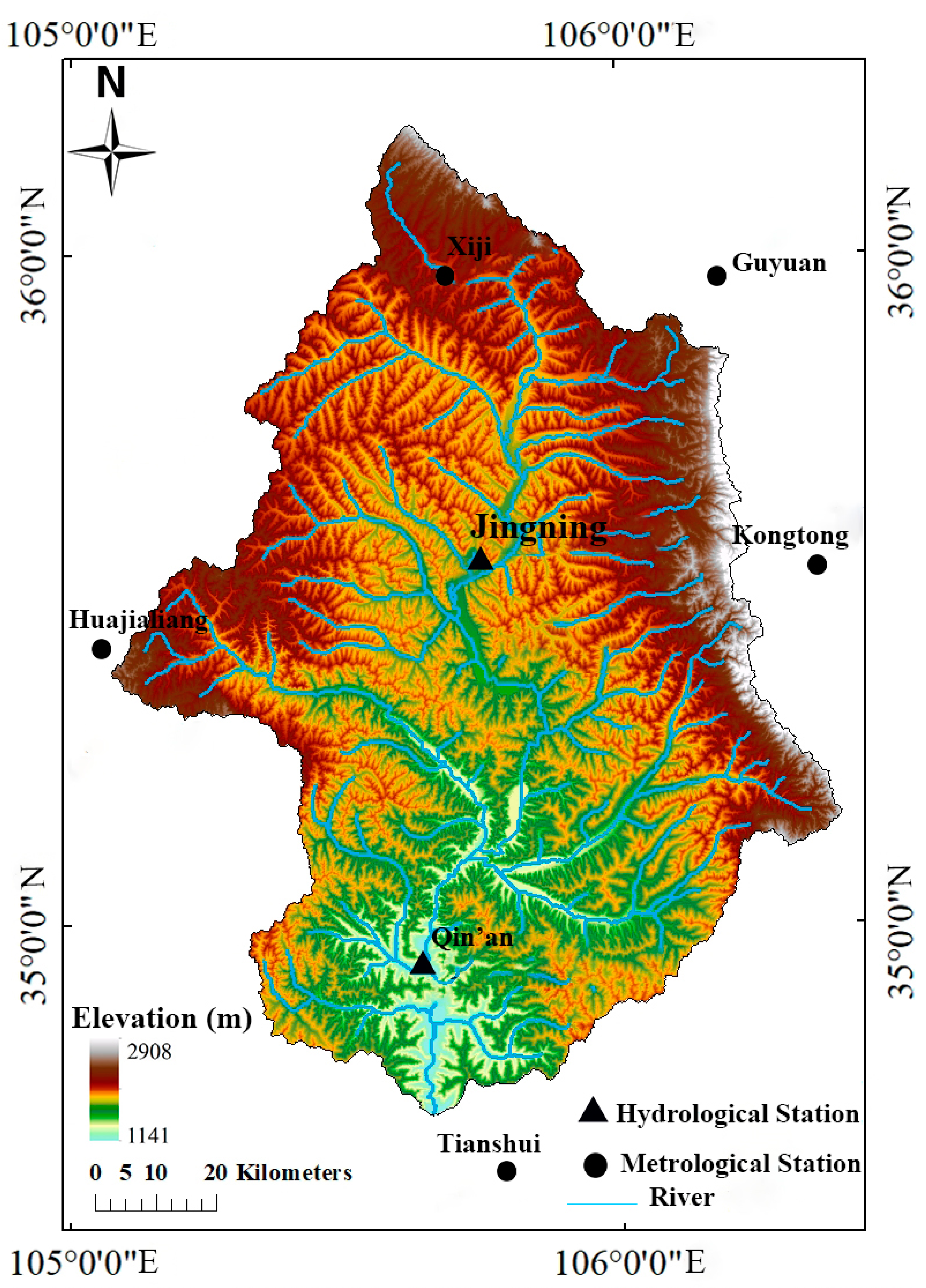
One of the major tributaries of the Wei River and the Hulu River rises on the southern slopes of Moon Mountain near the boundary between Xiji County and Haiyuan County in the Ningxia Hui Autonomous Region (Figure 1). The watershed is situated between 34°30′ and 36°30′ N and 105°05′ to 106°30′ E, and its height ranges from 1141 to 1908 m. According to [49], it crosses both the Ningxia Hui Autonomous Region and Gansu Province before emptying into the Wei River close to Tianshui City in Gansu Province. The research region has an east-west gradient with a higher north elevation and a lower south elevation. The riverbed resembles a gourd because it is meandering and has a wide range of widths [15]. The Hulu River’s main channel is 301 km long, and its entire basin is around 10,700 km2. With an annual sediment transfer as high as 7270 × 104 tons, the basin is characterized by significant vegetation destruction, loose soil, frequent heavy rainfall, and severe soil erosion. The Hulu River Basin’s water resources are dispersed unevenly and show noticeable inter-annual changes. A total of 265.4 million m3 of runoff are produced annually on average [49].
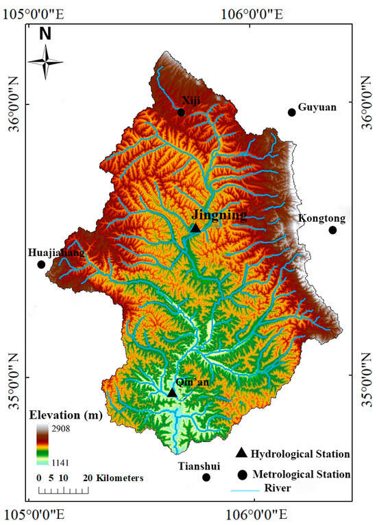
Figure 1.
DEM of the study area.
2.2. GAST Model
The GPU Accelerated Surface Water Flow and Transport Model (GAST) simulates basin flood response under various rainfall and land use scenarios using a numerical model that integrates hydrological and hydrodynamic processes. Its great accuracy, quick efficiency, and strong stability make it a good model for complicated networks. Urban waterlogging, sediment transport, and basin flood dynamics are among the processes it can accurately replicate. It can simulate these processes at a fine scale and use GPU-accelerated parallel computing technology, which greatly increases the model’s computational performance and offers several benefits [50].
2.2.1. Model Governing Equations
The GAST model utilizes the two-dimensional shallow water equations (SWEs) as the governing equations for surface runoff calculations. The conservation form of the vector equation (neglecting viscous terms of motion, turbulent viscous terms, wind stress, and Coriolis force) is shown in Equations (1)–(3) [51].
where t is the time, x and y are the Cartesian coordinates, and q is the flow variable vector made up of h, qx, and qy, which indicate water depth and unit-width discharges in the x and y directions, respectively; u and v are defined as depth-averaged velocities in the x and y directions, and it is evident that qx = uh and qy = vh; f and g are the flux vectors in the x and y directions; S is the source vector that only takes into account the slope source Sb and the friction source Sf; in this case, zb is the bed elevation and Cf is the bed roughness coefficient that is derived from the Manning coefficient n and h in the form of gn2/h1/3.
2.2.2. Numerical Methods of the Model
The two-dimensional hydrodynamic model GAST employs the Godunov finite volume method to solve the two-dimensional shallow water equations. Riemann’s approximate HLLC solver is used to calculate the mass flux and momentum flux at the cell interfaces [52]. The static water reconstruction method is used to handle negative water depths at dry–wet boundaries [53]. The bottom slope flux method is utilized to solve the variation in water depth [54]. An improved splitting-point implicit method is used for the frictional resistance source term to enhance computational stability [55]. A second-order explicit Runge–Kutta method is employed for time integration to ensure second-order accuracy [56]. The MUSCL scheme effectively addresses computational instabilities and non-conservation of mass and momentum caused by non-physical phenomena. Due to the large-scale study area and complex watershed in this study, GPU acceleration and parallel computing techniques are introduced, significantly enhancing the model’s computational efficiency to improve its computational speed further.
2.3. Model Setup and Validation
2.3.1. Input Data
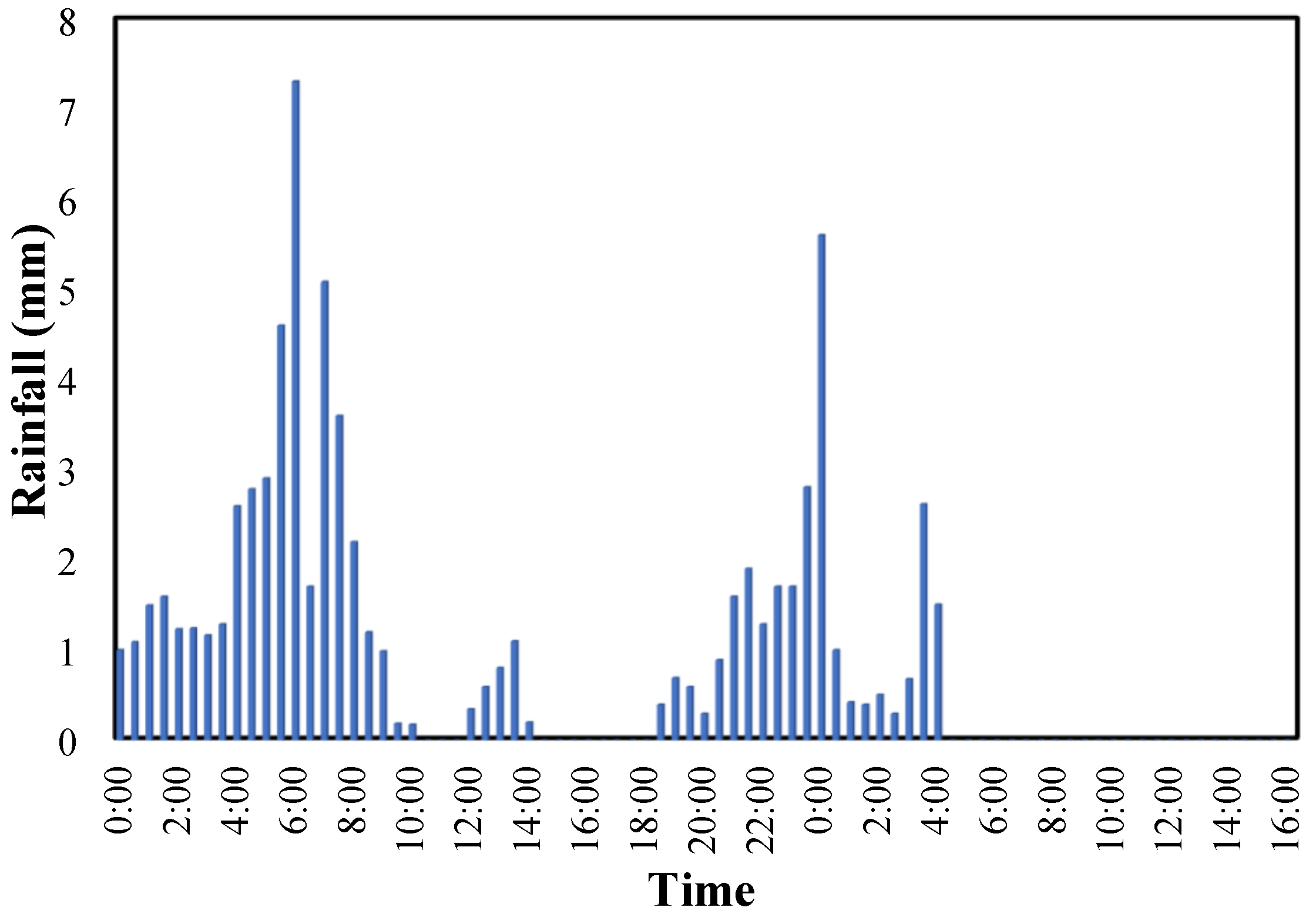
The primary input data for the GAST model are the digital elevation model (DEM), land use, soil, and meteorological data. River network features, topographic slope length, and other basin parameters are obtained using a digital elevation model (DEM). In this study, the China Meteorological Data Centre was used to compile rainfall data from the Hulu River Basin’s five meteorological stations, Huajialing, Tianshui, Kongtong, Guyuan, and Xiji. Observed rainfall data from 13 September 2019, 0:00 to 14 September 2019, 16:00 are used for model calibration and validation. The rainfall duration is 40 h, as shown in Figure 2. The time interval between data points is 30 min, and the simulation time is set to 40 h. Land use information from various historical eras was acquired from the Resource and Environmental Science and Data Centre of the Chinese Academy of Sciences. Data were collected with a resolution of 30 m for the years 1985–2020. Digital elevation model (DEM), land use information from various time periods, soil information, and precipitation information are among the fundamental data used in this study. The Geospatial Data Cloud (http://www.gscloud.cn/, accessed on 22 June 2023) provided the DEM data with a grid resolution of 30 m for download.
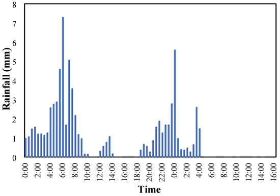
Figure 2.
Measured rainfall from 13 September 2019 at 0:00 to 14 September 2019 at 16:00.
The soil information was taken from the global Harmonized World Soil Database (HWSD), which was created by the Food and Agriculture Organization (FAO) and the International Institute for Applied Systems Analysis (IIASA). With a crop to the research area, the soil data are presented at a resolution of 1000 m. An analysis of the Hulu River Basin soil map was performed using the Harmonized World Soil Database (HWSD). The main soil types in the Hulu River Basin are saturated immature soil, unsaturated immature soil, calcareous accumulative black soil, moderately developed highly active leached soil, moderately developed black soil, moderately developed grey soil, moderately developed immature soil, calcareous impacted soil, calcareous immature soil, and sticky chestnut calcareous soil. In the basin, the predominant types of vegetation are cultivated land and grassland, with some woodland, bushes, unused land, water bodies, and impermeable regions also present [57]. The Horton infiltration model is used for the infiltration component of the model. In addition, the infiltration and Manning values for each land use type in the watershed are determined based on various references [58,59,60,61].
The commonly used infiltration equation, proposed by Horton in 1939, is as follows:
In this equation, the infiltration capacity at time t (h) is denoted by f, the starting value of infiltration capacity is represented by f0, the final or equilibrium infiltration capacity is represented by fc, and the rate of decline of infiltration capacity (1/h) is determined by an exponent k.
Horton used empirical methods to construct his equation, but it could also be theoretically determined if it were assumed that the decrease in infiltration capacity resulted from an exhaustion process [62].
2.3.2. Model Validation
This study utilizes measured rainfall and streamflow data from the Hulu River Basin to validate the accuracy and reasonability of the constructed GPU-accelerated Surface Water Flow and Associated Transport (GAST) model. The reliability of the model is assessed based on Nash–Sutcliffe Efficiency (NSE) and coefficient of determination (R2) for the flow at the watershed outlet cross-section. The downstream outlet of the Hulu River Basin in the GAST model is set as an open boundary, while the rest are set as closed boundaries. The model is validated using rainfall measured data from the Qin’an hydrological station from 13 September 2019 at 0:00 to 14 September 2019 at 16:00, spanning 40 h. The accuracy of the model is evaluated based on the root-mean-square error (RMSE) (Table 1) and relative error between the simulated values and measured values of the flow process at the Qin’an hydrological station.

Table 1.
Comparison between measured and simulated values.
2.3.3. Root Mean Square Error (RMSE)
In this equation: Qsim,i—simulated value, Qobs,i—observed value, and n—number of measurements. When the root-mean-square error (RMSE) is closer to 0, it indicates that the simulated values are in complete agreement with the observed values.
2.3.4. Relative Error
In the equations: δ—relative error, usually expressed as a percentage, △—difference between simulated and measured values, and L—measured value.
According to the calculations based on the simulation results, the root-mean-square error (RMSE) between the simulated and observed values is 3.98. The relative errors are 0.64%, 7.68%, 8.64%, 3.57%, 0.75%, and 3.33%, respectively. The RMSE is close to 0, and the relative errors are all less than 10%, indicating that the model has a small error between the simulated and observed values and exhibits high accuracy. Therefore, the model can be used to simulate and analyze the impact of rainfall characteristics and land use changes on flood events in the Hulu River Basin. Additionally, the average absolute value of the relative error is 0.0410, and the average absolute error is 3.1911.
2.4. Simulation of River Flooding under Different Rainfall Characteristics Scenarios
Different rainfall return periods have different impacts on basin floods, and the spatial distribution of rainfall, whether uniform or uneven, also significantly influences basin floods. Therefore, studying the impact of different rainfall spatial distributions on basin floods under different return periods can provide a theoretical basis for disaster prevention, mitigation, and relief work.
Scenario Setup
During the simulation period, the land use data in the Hulu River Basin are assumed to be the current land use while keeping the infiltration and other parameters constant to exclude the influence of other factors on the flood evolution process in the basin. The rainfall is designed using the Chicago rainfall type and the Gansu Tianshui rainfall formula. Short-duration intense rainfall with a rainfall duration of 120 min and return periods of 5 years, 10 years, and 50 years, respectively, is generated with a rain peak coefficient of 0.5. The rainfall formula is as follows:
In equations: i = rainfall intensity (mm/h), P = rainfall return period (years), and t—rainfall duration (minutes).
Two different scenarios are set for the spatial distribution of rainfall under different return periods. Based on the analysis of rainfall distribution and storm intensity distribution, it is known that the rainfall in the Hulu River Basin gradually decreases from southeast to northwest, with higher storm intensity in the southeast and northwest regions and lower intensity in the northeast and southwest regions. Therefore, two different rainfall spatial distribution scenarios are constructed. Additionally, three scenarios are created with the storm center located in the upstream, middle reaches and downstream regions. The specific settings for the rainfall characteristics scenarios are shown in Table 2.
Table 2.
Scenario setting of different rainfall characteristics.
2.5. Simulation of River Floods Occurance under Different Land Use Scenarios
Different land use types significantly impact the flood evolution process by altering the underlying surface hydrological characteristics, leading to a series of water resource issues such as increased flood disasters, severe soil erosion, and declining groundwater levels. In addition, changes in land use also have certain impacts on the ecological environment and economic conditions, such as implementing policies such as converting cultivated land to forests and grasslands in areas prone to soil erosion. Therefore, studying the impact of land use changes on watershed floods is important for disaster prevention and mitigation and provides technical support for watershed water resource planning. This section uses a two-dimensional hydrodynamic model to simulate and analyze the impact of land use changes in the Hulu River basin on the flood evolution process, peak flow, and peak water depths.
Scenario Setup
Since 1999, multiple water conservation measures have been implemented in the Hulu River basin. Therefore, a scenario of generalized water conservation measures (such as constructing sediment detention dams and terracing projects) is constructed. Seven land use scenarios are established, including the current land use scenario, three historical land use scenarios, two integrated land use scenarios, and the generalized water conservation measures scenario. The response of watershed floods under different land use scenarios is simulated and analyzed. The data for the four integrated land use scenarios are shown in Figure 3, and the specific scenario settings are shown in Table 3. To exclude the influence of rainfall on watershed floods, it is assumed that the rainfall conditions remain unchanged. The rainfall design adopts the Chicago rainfall pattern, and the Gansu Tianshui heavy rain formula (Equation (7)) is used to generate rainfall with a duration of 120 min and a rainfall coefficient of 0.5. The return periods are 5, 10, and 50 years, and the rainfall is assumed to be spatially uniformly distributed.
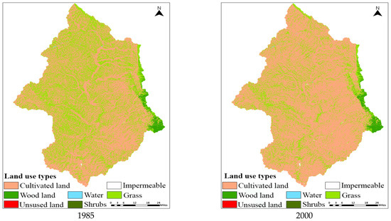

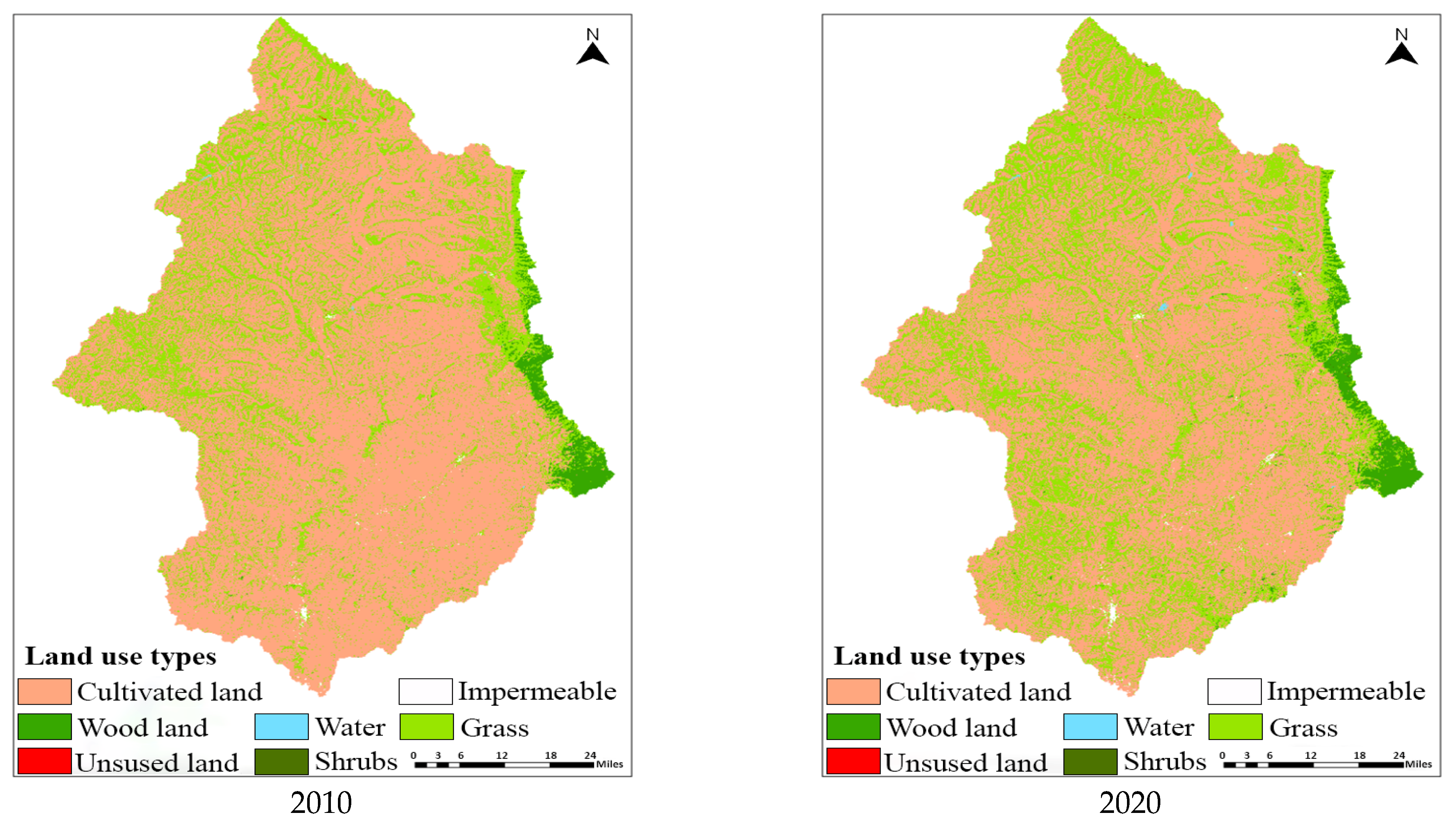
Figure 3.
The variation in land use pattern of the study area over time (1985–2020).
Table 3.
Set up different land use scenarios.
2.6. Simulation of River Floods under the Combined Influence of Rainfall Characteristics and Land Use
We integrate two influencing factors to simulate the impact of the combined changes in rainfall characteristics and land use on watershed floods. We explore the patterns and characteristics of changes in peak flow and peak water depth.
Scenario Setup
Based on the analysis in the previous section, it was found that the impact of the rainfall center on watershed floods is similar in the upstream and middle reaches of the watershed. Therefore, in this section, besides other scenarios of rainfall characteristics, only the scenario with the rainfall center upstream of the watershed was selected for simulation. The specific scenario settings are shown in Table 4.
Table 4.
Scenario setting under the combined action of rainfall characteristics and land use.
3. Results
Rainfall and land use are intricately interconnected, influencing each other in several significant ways. The changes that occur in land use, such as urbanization or deforestation, can alter the natural water cycle, impacting both the intensity and rainfall distribution. Conversely, rainfall patterns influence land use decisions, especially in agriculture, where the amount and timing of precipitation often dictate the choice of crops and farming practices. This dynamic relationship highlights the importance of considering both environmental planning and resource management factors.
3.1. Simulation of River Flooding under Different Rainfall Characteristics Scenarios
Rainfall return periods of 5, 10, and 50 years with uniform spatial distribution of rainfall. The flood evolution process under different return periods with a uniform spatial rainfall distribution was simulated. The hydrograph, peak flow, and peak water depth at the outlet section of the basin under different return periods with a uniform spatial distribution of rainfall are shown in Figure 4 and Table 5.

Figure 4.
Different rainfall return periods under uniform rainfall distribution. (a) Scenario R1; (b) Scenario R2; and (c) Scenario R3.
Table 5.
Peak discharge and peak water depth under different spatial distributions of rainfall.
Figure 4 shows that the flow at the outlet section of the basin rapidly increases with time, reaching its peak between 5400 s and 7200 s, and then slowly decreases to a stable level. Both scenario R1 and scenario R2 exhibit a flow value close to the peak flow, which can occur either before or after the peak flow. Scenario R3, on the other hand, does not show a flow value close to the peak flow. Instead, it experiences a sudden drop after the peak flow, followed by a subsequent rise and a slow decline to stability. The peak flow in scenario R1 is 1332.90 m3/s, occurring at 7200 s, with a peak water depth of 5.42 m at 9000 s. In scenario R2, the peak flow is 1445.33 m3/s, occurring at 5400 s, with a peak water depth of 5.44 m at 9000 s. Scenario R3 has a peak flow of 2003.04 m3/s, occurring at 5400 s, with a peak water depth of 8.57 m at 9000 s. It can be observed that both the peak flow and peak water depth increase with the increase in the return period. However, when the return periods are relatively close, such as 5 years and 10 years, the increase in peak flow and peak water depth is not significant. Furthermore, as the return period increases, the timing of the peak flow advances. There will be changes in future precipitation due to global warming and the intensification of the water cycle process [63,64].
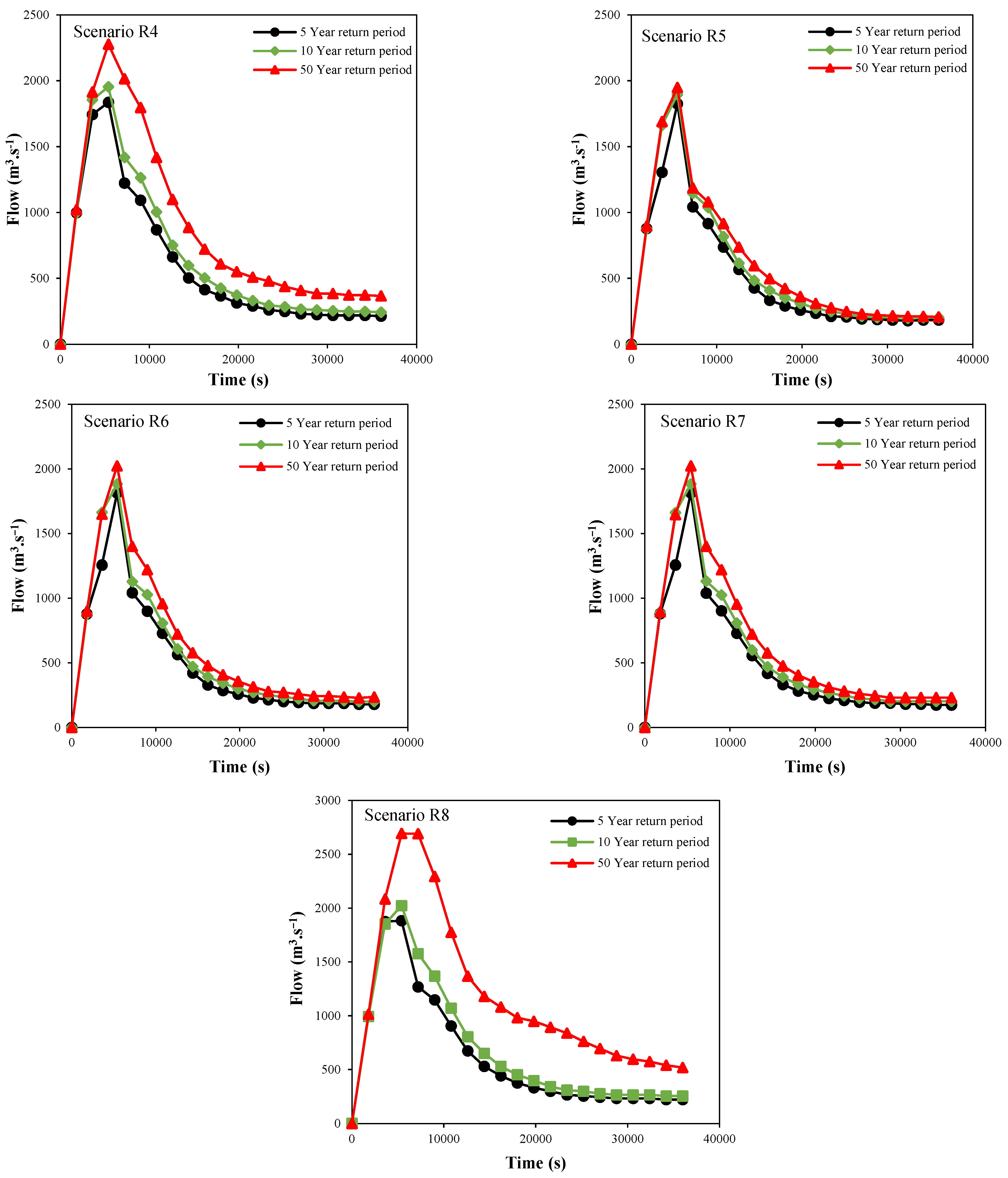
The spatial distribution of rainfall is uneven, with a return period of 5, 10, and 50 years. Simulate the flood evolution process under different return periods of uneven rainfall. The flow hydrograph, peak flow, and peak water depth of the watershed outlet section under different return periods of uneven rainfall are shown in Figure 5 and Table 6. Scenario R4 and Scenario R8 have significant differences in the discharge hydrograph of the watershed outlet section at different return periods, while Scenario R5, Scenario R6, and Scenario R7 have little difference in the discharge hydrograph of the outlet section at different return periods. The peak flow rates of scenarios R4, R5, R6, and R7 with different return periods all appeared at 5400 s and then gradually decreased with time. The peak flow of scenario R8 with different return periods occurs between 5400 s and 7200 s and then slowly decreases to a stable state. The outlet section discharge hydrograph of scenario R6 and scenario R7 is not very different; that is, when the rainfall center is in the upstream and midstream, the impact on the basin flood is relatively close. Scenario R8 is quite different from scenarios R6 and R7, which indicates that when the rainfall center is downstream, the impact on the basin flood is different from that in the middle and upstream.

Figure 5.
The flow process line of the basin outlet section is under different uneven rainfall distributions.
Table 6.
Peak flow and peak water depth under different rainfall scenarios.
Scenario R4 has a peak flow rate of 1836.19 m3/s, 1954.21 m3/s, and 2277.76 m3/s during the 5, 10, and 50-year return periods, respectively, which is 37.76%, 35.21%, and 13.72% higher than the uniform distribution of rainfall during the same return period. The peak water depths are 5.38 m, 5.41 m, and 7.39 m, respectively, 0.74%, 0.55%, and 13.77% less than the uniform rainfall distribution. Scenario R5 has a peak flow rate of 1825.59 m3/s, 1894.72 m3/s, and 1949.12 m3/s under three different return periods, respectively. Compared with the same return period, the rainfall distribution uniformly increased by 36.96%, 31.09%, and decreased by 2.69%. The peak water depths were 5.61 m, 5.39 m, and 5.40 m, respectively, which increased by 3.51%, decreased by 0.92%, and 36.99% compared to the uniform distribution of rainfall. Scenario R6 has a peak flow rate of 1813.82 m3/s, 1883.36 m3/s, and 2023.07 m3/s during the 5, 10, and 50-year return periods, respectively, which is 36.08%, 30.31%, and 1.00% higher than the uniform distribution of rainfall during the same return period; The peak water depths were 5.60 m, 5.39 m, and 5.86 m, respectively, which increased by 3.32%, decreased by 0.92%, and 31.62% compared to the uniform distribution of rainfall.
Scenario R7 has a peak flow rate of 1813.73 m3/s, 1883.31 m3/s, and 2023.22 m3/s during the 5, 10, and 50-year return periods, respectively, which is 36.07%, 30.30%, and 1.01% higher than the uniform distribution of rainfall during the same return period. The peak water depths were 5.60 m, 5.39 m, and 5.86 m, respectively, which increased by 3.32%, decreased by 0.92%, and 31.62% compared to the uniform distribution of rainfall. Scenario R8 has a peak flow rate of 1883.34 m3/s, 2023.48 m3/s, and 2694.34 m3/s during the 5, 10, and 50-year return periods, respectively, which is 41.30%, 40.00%, and 34.51% higher than the uniform distribution of rainfall during the same return period. The peak water depths were 5.39 m, 5.71 m, and 8.82 m, respectively, which decreased by 0.55%, increased by 4.96%, and 2.92% compared to the uniform distribution of rainfall.
Figure 5 shows that the peak flow values and peak water depths for the 5-year and 10-year return periods are relatively close across different scenarios, while there is a significant difference between the 10-year and 50-year return periods. It is quite different from the peak water depth. It is further explained that when the difference between return periods is larger, the difference between peak flow rate and peak water depth is larger. The peak flow and peak water depth under the above four scenarios with uneven rainfall spatial distribution are quite different from those under uniform rainfall spatial distribution. The largest difference is scenario R8, and the one closest to the uniform rainfall scenario is scenario R7. It can be seen that when the return period is small, the change rate of peak flow is larger, and when the return period is larger, the change rate of peak flow is smaller. It can be seen that when the return period reaches a certain level, such as the 100-year return period, the peak discharge at the outlet section of the basin is relatively close under the scenarios of uneven rainfall distribution and uniform rainfall distribution.
The simulated peak flows of Scenario R4, Scenario R5, Scenario R6, and Scenario R7 under the 5-year return period are relatively close, indicating that when the return period is small, the heavy rain center is in the southeast, southeast, and northwest, the upper reaches of the basin and the middle reaches of the basin. The degree of flood impact in the Hulu River Basin is relatively similar. The peak flows simulated by scenario R8 are significantly different from those of other scenarios in all return periods, indicating that when the center of heavy rain is in the lower reaches of the basin, the impact on floods in the basin is stronger. At this time, special attention should be paid to the safety of the rivers downstream of the basin, and disaster prevention and reduction measures should be taken.
3.2. Simulation of River Flooding under Different Land Use Scenarios
The historical inversion method is used to simulate the four historical land use scenarios, and the changes in the simulation results between two adjacent periods are considered as the degree of land use impact on floods. The peak flow and peak water depth for different return periods under each scenario are shown in Table 7 and Table 8, respectively. The flood hydrographs at the watershed outlet for different land use scenarios are shown in Figure 6.
Table 7.
Historical land use scenarios peak discharge and peak water depth.
Table 8.
Peak discharge and peak water depth in comprehensive land use scenarios.
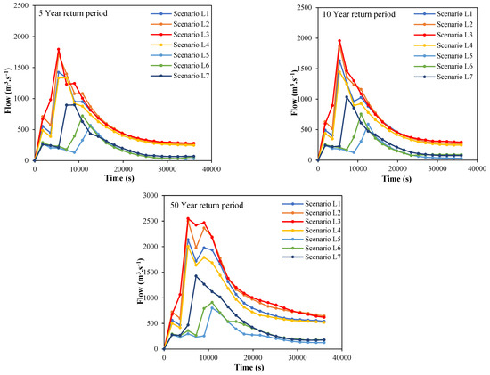
Figure 6.
Flow process line of watershed outlet section under different land use scenarios.
Table 7 shows that compared to Scenario L1, Scenario L2 shows an increase in peak flow of 20.26%, 14.68%, and 17.14% for the 5, 10, and 50-year return periods, respectively. The peak water depth increases by 0.37%, 9.07%, and 3.80%, respectively. Compared to Scenario L2, Scenario L3 shows an increase in peak flow of 4.92%, 4.72%, and 1.86%, and an increase in peak water depth of 1.66%, 6.62%, and 2.63% for the 5, 10, and 50-year return periods, respectively. Compared to Scenario L3, Scenario L4 shows a decrease in peak flow of 25.75%, 26.18%, and 21.39%, and a decrease in peak water depth of 1.45%, 13.38%, and 4.57% for the 5, 10, and 50-year return periods, respectively. It can be observed that there is a significant variation in peak flow between two adjacent land use scenarios, while the variation in peak water depth is less than 15%. This indicates that the changes in land use between two adjacent periods have a greater impact on peak flow and a relatively smaller impact on peak water depth.
In Scenario L1 compared to Scenario L4, the peak flow increased by 6.74%, 12.80%, and 6.62% for different return periods, while the peak water depth decreased by 0.55%, 0.74%, and 1.63% for the 5, 10, and 50-year return periods, respectively. In Scenario L2 compared to Scenario L4, the peak flow increased by 28.37%, 29.36%, and 24.89% for different return periods, and the peak water depth decreased by 0.18% for the 5-year return period but increased by 8.27% and 2.10% for the 10 and 50-year return periods, respectively. In Scenario L3 compared to Scenario L4, the peak flow increased by 34.68%, 35.47%, and 27.22% for the 5, 10, and 50-year return periods, respectively, and the peak water depth increased by 1.48%, 15.44%, and 4.78% for the corresponding return periods. Thus, it can be observed that during the period from 1985 to 2020 [65,66], the changes in land use resulted in an increasing trend followed by a decreasing trend in both peak flow and peak water depth in the watershed.
The flood evolution process was simulated and analyzed for three land use scenarios, including two integrated land use scenarios and one scenario considering generalized water conservation measures, compared to the current land use scenario (Scenario L4). The simulation results and the changes compared to the current land use scenario are shown in Table 8. From the table, it can be seen that the peak flow differs significantly among the two integrated land use scenarios and the scenario with generalized water conservation measures for different return periods, while the variation in peak water depth is relatively small. Compared to Scenario L4, the peak flow decreased by 57.34%, 45.92%, and 32.63% for the 5-year return period in Scenarios L5, L6, and L7, respectively. Similarly, for the 10-year and 50-year return periods, the peak flow decreased by 59.19%, 47.73%, 28.33%, and 59.91%, 54.46%, and 28.79%, respectively. The corresponding reductions in peak water depth were 11.62%, 9.04%, and 2.95% for the 5-year return period, 11.76%, 8.64%, and 2.57% for the 10-year return period, and 41.89%, 40.49%, and 35.47% for the 50-year return period.
Furthermore, according to Figure 6, the peak flow in Scenarios L5, L6, and L7 occurs later than in Scenario L4, approximately between 3600 s and 7200 s. This indicates that not only do the peak flow and peak water depth decrease significantly for different return periods, but they also occur later. It suggests that the measures of returning farmland to forest and grassland have a pronounced inhibitory effect on both peak flow and peak water depth. The water conservation measures also contribute to a delay in peak flow and peak water depth. This is because the implementation of water conservation measures retains most of the runoff locally, leading to a decreasing trend in peak flow and peak water depth at the outlet section of the watershed.
The main land use types in the Hulu River Basin are cultivated land and grassland, supplemented by woodland, shrubs, water bodies, unused land, and impermeable areas. Cultivated land has the highest proportion in all four periods, exceeding 60% and being the largest land use type. Grassland has the second largest proportion, also exceeding 20%. In these four periods, the proportion of arable land shows a trend of first increasing and then decreasing, accounting for 60.09%, 75.62%, 72.94%, and 62.66% of the total area, respectively. The proportion of grassland shows a trend of decreasing first and then increasing, accounting for 38.02%, 22.30%, 24.78%, and 34.10%, respectively. The proportion of woodland gradually increases, accounting for 1.71%, 1.89%, 2.04%, and 2.81%, respectively. The proportion of shrubs shows a slight increase, accounting for 0.009%, 0.006%, 0.005%, and 0.017% of the total area. The proportion of water bodies and unused land initially decreases and then increases, while the proportion of impermeable areas gradually increases. Between 1985 and 2020, except for a 3.92% decrease in grassland area, the area of cultivated land, woodland, shrubs, water bodies, unused land, and impermeable areas all increased. The increase in proportion is 2.57%, 1.10%, 0.01%, 0.05%, 0.01%, and 0.18%, respectively. In short, the Hulu River Basin has been mainly characterized by cultivated land and grassland, with increasing proportions of woodland and shrubs. Water bodies, unused land, and impermeable areas have also shown changes in their proportions (Table 9).
Table 9.
The land use change occurred in the study area during the period 1985–2020.
3.3. Simulating the Interacting Effects of Rainfall and Land Use Characteristics on River Flooding
By taking the peak flow and peak water depth obtained from the simulation of the 50-year return period uniform rainfall and land use scenario as the baseline and comparing and analyzing the simulation results under different comprehensive scenarios, we can determine the degree of impact of the combined changes in rainfall characteristics and land use on floods. The simulation results for scenarios RL1-1 to RL1-6 are shown in Table 10, and the outflow hydrographs are shown in Figure 7a. The peak flow occurs at 5400 s for all scenarios. In scenario RL1-1, the peak flow is 2313.54 m3/s, and the peak water depth is 7.47 m, representing a 15.50% increase in peak flow and a 12.84% decrease in peak water depth compared to the baseline period. In scenario RL1-2, the peak flow is 2377.32 m3/s, representing an 18.69% increase, and the peak water depth is 8.17 m, representing a 4.67% decrease. In scenario RL1-3, the peak flow is 2424.66 m3/s, and the peak water depth is 8.36 m, representing a 21.05% increase in peak flow and a 2.45% decrease in peak water depth compared to the baseline period. In scenario RL1-4, the peak flow is 1902.56 m3/s, and the peak water depth is 5.39 m, representing a 5.02% decrease in peak flow and a 37.11% decrease in peak water depth compared to the baseline period. In scenario RL1-5, the peak flow is 2002.31 m3/s, and the peak water depth is 5.42 m, representing a 0.04% decrease in peak flow and a 36.76% decrease in peak water depth compared to the baseline period. In scenario RL1-6, the peak flow is 2277.76 m3/s, and the peak water depth is 7.39 m, representing a 13.72% increase in peak flow and a 13.77% decrease in peak water depth compared to the baseline period.
Table 10.
Scenarios RL1-1 to RL1-6 peak flow rate and peak water depth.
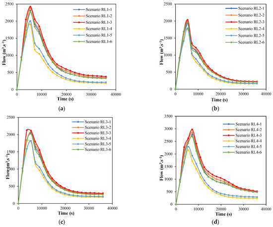
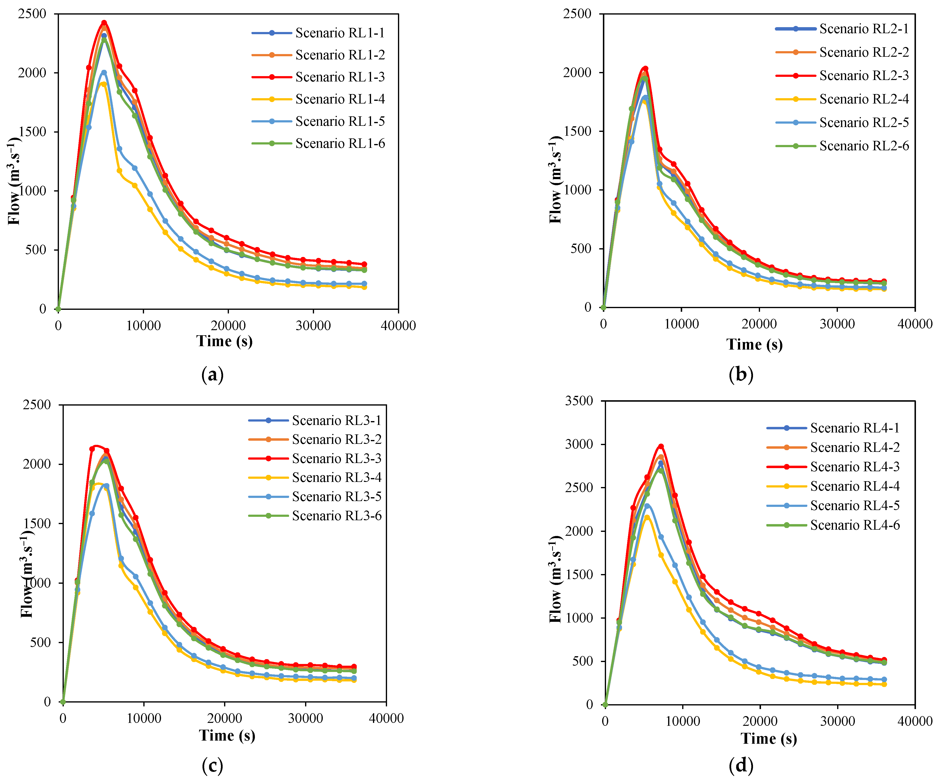
Figure 7.
Flow process line of basin outlet section under different comprehensive scenarios. (a) Scenario RL1; (b) Scenario RL2; (c) Scenario RL3; (d) Scenario RL4 figure.
The simulation results for scenarios RL2-1 to RL2-6 are shown in Table 11, and the outflow hydrographs are shown in Figure 7b. The peak flow occurs at 5400 s for all scenarios. In scenario RL2-1, the peak flow is 1989.97 m3/s, and the peak water depth is 5.42 m, representing a 0.65% decrease in peak flow and a 36.76% decrease in peak water depth compared to the baseline period. In scenario RL2-2, the peak flow is 1990.56 m3/s, representing a 0.62% decrease, and the peak water depth is 5.41 m, representing a 36.87% decrease. In scenario RL2-3, the peak flow is 2033.76 m3/s, and the peak water depth is 5.55 m, representing a 1.53% increase in peak flow and a 35.24% decrease in peak water depth compared to the baseline period. In scenario RL2-4, the peak flow is 1751.75 m3/s, and the peak water depth is 5.34 m, representing a 12.55% decrease in peak flow and a 37.69% decrease in peak water depth compared to the baseline period. In scenario RL2-5, the peak flow is 1786.75 m3/s, and the peak water depth is 5.34 m, representing a 10.80% decrease in peak flow and a 37.69% decrease in peak water depth. In scenario RL2-6, the peak flow is 1947.12 m3/s, and the peak water depth is 5.40 m, representing a 2.79% decrease in peak flow and a 36.99% decrease in peak water depth compared to the baseline period.
Table 11.
Scenarios RL2-1 to RL2-6 peak flow rate and peak water depth.
The simulation results for scenarios RL3-1 to RL3-6 are shown in Table 12, and the outflow hydrographs are shown in Figure 7c. The peak flow occurs between 3600 s and 5400 s for all scenarios. In scenario RL3-1, the peak flow is 2052.46 m3/s, and the peak water depth is 5.90 m, representing a 2.47% increase in peak flow and a 31.16% decrease in peak water depth compared to the baseline period. In scenario RL3-2, the peak flow is 2088.33 m3/s, representing a 4.26% increase, and the peak water depth is 6.21 m, representing a 27.54% decrease. In scenario RL3-3, the peak flow is 2127.37 m3/s, and the peak water depth is 6.49 m, representing a 6.21% increase in peak flow and a 24.27% decrease in peak water depth compared to the baseline period. In scenario RL3-4, the peak flow is 1796.61 m3/s, and the peak water depth is 5.34 m, representing a 10.31% decrease in peak flow and a 37.69% decrease in peak water depth compared to the baseline period. In scenario RL3-5, the peak flow is 1817.12 m3/s, and the peak water depth is 5.36 m, representing a 9.28% decrease in peak flow and a 37.46% decrease in peak water depth. In scenario RL3-6, the peak flow is 2023.07 m3/s, and the peak water depth is 5.71 m, representing a 1.00% increase in peak flow and a 33.37% decrease in peak water depth compared to the baseline period.
Table 12.
Scenarios RL3-1 to RL3-6 peak flow rate and peak water depth.
The simulation results for scenarios RL4-1 to RL4-6 are shown in Table 13, and the discharge hydrograph at the outlet cross-section is shown in Figure 7d. The peak flow occurs between 5400 s and 7200 s. In scenario RL4-1, the peak flow is 2783.00 m3/s, and the peak water depth is 8.81 m. Compared to the baseline period, the peak flow has increased by 38.94%, and the peak water depth has increased by 2.80%. In scenario RL4-2, the peak flow is 2853.87 m3/s, an increase of 42.48% compared to the baseline period, and the peak water depth is 8.82 m, which is an increase of 2.92%. In scenario RL4-3, the peak flow is 2974.82 m3/s, and the peak water depth is 9.0 m. These values represent an increase of 48.52% and 5.02%, respectively, compared to the baseline period. In scenario RL4-4, the peak flow is 2156.24 m3/s, and the peak water depth is 5.91 m. The peak flow has increased by 7.65%, while the peak water depth has decreased by 31.04% compared to the baseline period. In scenario RL4-5, the peak flow is 2289.18 m3/s, and the peak water depth is 6.87 m. The peak flow has increased by 14.29%, while the peak water depth has decreased by 19.84% compared to the baseline period. In scenario RL4-6, the peak flow is 2694.34 m3/s, and the peak water depth is 8.82 m. The peak flow has increased by 34.51%, and the peak water depth has increased by 2.92% compared to the baseline period.
Table 13.
Scenarios RL4-1 to RL4-6 peak traffic and peak water depth.
The variations between scenarios RL1-1 to RL1-6, RL2-1 to RL2-6, RL3-1 to RL3-6, and RL4-1 to RL4-6 represent the influence of land use changes on watershed flooding. The range of variation in peak flow is 1.55% to 21.53%, 0.03% to 13.87%, 1.14% to 15.55%, and 2.55% to 27.52%, respectively. The range of variation in peak water depth is 0.56% to 37.11%, 0.00% to 3.78%, 0.37% to 17.72%, and 0.00% to 49.24%, respectively. When the rainfall gradually decreases from southeast to northwest, and the rainfall center is located downstream, the impact of land use changes on watershed flooding is significant, while in the other two land use scenarios, the impact is relatively small.
The variations between scenarios RL1-1, RL2-1, RL3-1, and RL4-1, RL1-2, RL2-2, RL3-2, and RL4-2, RL1-3, RL2-3, RL3-3, and RL4-3, RL1-4, RL2-4, RL3-4, and RL4-4, RL1-5, RL2-5, RL3-5, and RL4-5, RL1-6, RL2-6, RL3-6, and RL4-6 represent the influence of changes in rainfall characteristics on peak flow and peak water depth. The range of variation in peak flow is 3.14% to 39.85%, 4.91% to 43.37%, 4.60% to 46.27%, 2.56% to 23.09%, 1.70% to 28.12%, and 3.90% to 38.38%, respectively. The range of variation in peak water depth is 8.86% to 62.55%, 7.96% to 63.03%, 7.66% to 62.16%, 0.00% to 10.67%, 0.37% to 28.65%, and 5.74% to 63.33%, respectively. When the land use scenario is afforestation and grassland restoration, the impact of changes in rainfall characteristics on watershed flooding is relatively small, while in the other land use scenarios, the impact is more significant. Therefore, except for the land use scenario of afforestation and grassland restoration in the entire region, rainfall characteristics have a greater impact on watershed flooding than land use changes.
In short, it is stated that the most unfavorable scenario for the Hulu River Basin in terms of rainfall characteristics and land use is scenario RL4-3, with a peak flow rate of 2974.82 m3/s and a peak water depth of 9.00 m. In this scenario, the rainfall distribution is concentrated in the downstream area, and the land use corresponds to the land use in 2010. The basin is threatened by severe floods not only due to changes in rainfall distribution but also because of the reduction in grassland and forest land and the increase in cultivated land.
On the other hand, the scenario with the greatest reduction in flood risk due to rainfall characteristics and land use is RL2-4, with a peak flow rate of 1751.75 m3/s and a peak water depth of 5.34 m. In this scenario, the rainfall is heavier in the southeast and northwest regions and lighter in the northeast and southwest regions. The land use type is characterized by reforestation and the return of cultivated land to forests. The changes in rainfall distribution and the increase in grassland contribute to the decrease in flood threat.
4. Discussion
The GAST model was found to be suitable for investigating the Impacts Assessment of Rainfall Characteristics and Land use Patterns on Runoff accumulation in the Hulu River Basin, China. Overall, the GAST model performance classification for the watershed was very good [67]. The GAST model results revealed that rainfall and land use had an effect on the hydrologic process of the Hulu River basin. The observed changes in hydrological processes were attributed to rainfall and land use changes for this study.
4.1. Flood Evolution under Different Rainfall Characteristics Scenarios
With uniform rainfall distribution, an increase in the return period leads to higher peak flow rates and peak water depths, and the occurrence time of peak flow advances. When the difference in return periods is small, such as 5 and 10-year return periods, the increase in peak flow rates and peak water depths is not significant. However, when the rainfall distribution is non-uniform, there is a considerable difference in peak flow rates and peak water depths compared to the scenario with uniform rainfall distribution. As the return period increases, the impact of non-uniform rainfall distribution on peak flow rates decreases. Among the scenarios, scenario R8 has the greatest impact on basin floods. Under a 5-year return period, the peak flow rate increases by 41.30%, and the peak water depth decreases by 0.55%. Under a 10-year return period, the peak flow rate increases by 40.00%, and the peak water depth increases by 4.96%. Under a 50-year return period, the peak flow rate increases by 34.51%, and the peak water depth increases by 2.92%. The scenario that is closest to the uniform rainfall scenario is R7, with a 36.07% increase in peak flow rate and a 3.22% increase in peak water depth under a 5-year return period, a 30.30% increase in peak flow rate and a 0.92% decrease in peak water depth under a10-year return period, and a 1.01% increase in peak flow rate and a 33.37% decrease in peak water depth under 50-year return period.
4.2. Flood Evolution Process under Different Land Use Scenarios
Different land use scenarios result in varying responses in peak flow rates and peak water depths. From 1985 to 2020, the changes in land use led to an initial increase and subsequent decrease in peak flow rates and peak water depths in the Hulu River Basin. Compared to the current land use in 2020, all three historical land use scenarios resulted in increased peak flow rates, while the peak water depths showed variations. Scenario L1 leads to a decrease in peak water depth compared to the current land use scenario. In scenario L2, the peak water depth is smaller under a 5-year return period, while it increases under 10-year and 50-year return periods compared to the current scenario. Scenario L3 results in increased peak water depths compared to the current land use scenario. The integrated land use scenarios and generalized water conservation measures lead to significant differences in peak flow rates compared to the current land use scenario. Across different return periods, there is a significant decrease in peak flow rates, and the occurrence time is delayed. The magnitude of the impacts on peak flow rates and peak water depths is as follows: L5 > L6 > L7.
4.3. Flood Evolution under the Combined Influence of Different Rainfall Characteristics and Land Use
The combined effect of rainfall characteristics and land use has the greatest impact on basin floods in scenario RL4-3, where the rainfall center is located downstream, and the land use corresponds to the 2010 land use type. The resulting peak flow rate and peak water depth are 2974.82 m3/s and 9.00 m, respectively. The range of the impacts of land use changes on basin floods is between 0.04% and 48.52%, while the range of changes in peak flow rates and peak water depths due to rainfall characteristics is between 0.00% and 63.33%. Under the combined effect of rainfall characteristics and land use changes, the range of changes in peak flow rates and peak water depths is between 0.04% and 48.52%. In general, except for the scenarios with region-wide reforestation and grassland restoration land use, the impact of rainfall characteristic changes on basin floods is greater than the impact of land use changes.
5. Conclusions
In this study, a two-dimensional hydrodynamic GAST model (GPU Accelerated Surface Water Flow and Transport Model) is set up to simulate the flood processes in the Hulu River Basin under different rainfall characteristics and land use scenarios. The impacts of various rainfall and land use scenarios on peak flow rates, peak water depths, and flood propagation processes were analyzed and quantified. In the Hulu River Basin, rainfall distribution and land use significantly affect peak flow and water depth. Uniform rainfall increases peak flow and depth, especially during longer return periods, while uneven rainfall lessens this impact. Concentrated rainfall poses the greatest flood risk in downstream areas, necessitating early emergency response and disaster plans. Land use changes from 1985 to 2020 influenced these patterns, with peak flow initially increasing and then decreasing. Shifting land use towards forestry and grassland and implementing soil and water conservation measures showed a notable decrease in runoff. Future efforts should focus on rainfall prediction and land use policy implementation to mitigate flood risks effectively.
The GAST model developed can predict the river basin’s future streamflow conditions. It can guarantee the sustainable use of water resources and provide a theoretical foundation for the planning and management of the total amount of simulated streamflow of water resources in large river basins and regions.
6. Policy Implications
Based on the context provided by the hydrodynamic model GAST and its accuracy assessment through RMSE. It can be used for flood forecasting and management. The model’s outputs could inform infrastructure development policies, such as where to build flood defenses or how to design them to withstand predicted flow rates. Policies related to environmental protection might be impacted if the flow simulations suggest changes in water patterns that could affect ecosystems. The research may have implications for urban planning policies. Flood prediction could affect agricultural areas and may lead to changes in agricultural policies, such as crop insurance schemes or water management practices. In summary, the policy implications of a hydrodynamic model simulation study are vast and can influence a wide range of policy areas, from local urban planning to broader environmental and risk management strategies.
Author Contributions
M.I. conceived the conceptualization of the research study, design and development of the experiment, data collection, formal analysis, investigation, methodology, visualization, writing an original draft, reviewed, supervised, and write-up editing. T.W., D.L., X.G., R.S.N., J.J. and M.A. contributed to the review and editing of the draft. J.H. supervised the entire research study and contributed as an internal reviewer for the manuscript. All authors have read and agreed to the published version of the manuscript.
Funding
This research was supported by National Natural Science Foundation of China (52079106, 52009104). Science and Technology Projects of Northwest Engineering Corporation Limited, Power China (XBY-ZDKJ-2022-9).
Data Availability Statement
Data is contained within the article.
Acknowledgments
The authors are thankful and acknowledge the State Key Laboratory of Eco-hydraulics in the Northwest Arid Region of China, Xi’an University of Technology, Xi’an 710048, Shaanxi, China.
Conflicts of Interest
Author Xujun Gao was employed by the company Power China Northwest Engineering Corporation Limited. The remaining authors declare that the research was conducted in the absence of any commercial or financial relationships that could be construed as a potential conflict of interest.
References
- Wang, X.; Zhang, P.; Liu, L.; Li, D.; Wang, Y. Effects of human activities on hydrological components in the Yiluo River basin in middle Yellow River. Water 2019, 11, 689. [Google Scholar] [CrossRef]
- Zhan, C.; Jiang, S.; Sun, F.; Jia, Y.; Niu, C.; Yue, W. Quantitative contribution of climate change and human activities to runoff changes in the Wei River basin, China. Hydrol. Earth Syst. Sci. 2014, 18, 3069–3077. [Google Scholar] [CrossRef]
- Allen, M.R.; Ingram, W.J. Constraints on future changes in climate and the hydrologic cycle. Nature 2002, 419, 224–232. [Google Scholar] [CrossRef] [PubMed]
- Wang, G.; Xia, J.; Chen, J. Quantification of effects of climate variations and human activities on runoff by a monthly water balance model: A case study of the Chaobai River basin in northern China. Water Resour. Res. 2009, 45, W00A11. [Google Scholar] [CrossRef]
- Wang, S.; Yan, M.; Yan, Y.; Shi, C.; He, L. Contributions of climate change and human activities to the changes in runoff increment in different sections of the Yellow River. Quat. Int. 2012, 282, 66–77. [Google Scholar] [CrossRef]
- Xu, C.-Y. Climate change and hydrologic models: A review of existing gaps and recent research developments. Water Resour. Manag. 1999, 13, 369–382. [Google Scholar] [CrossRef]
- Sharma, C.S.; Behera, M.D.; Mishra, A.; Panda, S.N. Assessing flood induced land-cover changes using remote sensing and fuzzy approach in Eastern Gujarat (India). Water Resour. Manag. 2011, 25, 3219–3246. [Google Scholar] [CrossRef]
- Suwanwerakamtorn, R. Register | Login. ITC J. 1994, 4, 343–348. [Google Scholar]
- Brooks, K.N.; Ffolliott, P.F.; Gregersen, H.M.; Thames, J. Hydrology and the Management of Watersheds; Iowa State University Press: Ames, IA, USA, 1991. [Google Scholar]
- Fohrer, N.; Haverkamp, S.; Eckhardt, K.; Frede, H.-G. Hydrologic response to land use changes on the catchment scale. Phys. Chem. Earth Part B Hydrol. Ocean. Atmos. 2001, 26, 577–582. [Google Scholar] [CrossRef]
- Liu, J.; Wang, S.-Y.; Li, D.-M. The analysis of the impact of land-use changes on flood exposure of Wuhan in Yangtze River Basin, China. Water Resour. Manag. 2014, 28, 2507–2522. [Google Scholar] [CrossRef]
- Chen, D.; Lu, X.; Hu, W.; Zhang, C.; Lin, Y. How urban sprawl influences eco-environmental quality: Empirical research in China by using the Spatial Durbin model. Ecol. Indic. 2021, 131, 108113. [Google Scholar] [CrossRef]
- Ahmadi, A.; Aghakhani Afshar, A.; Nourani, V.; Pourreza-Bilondi, M.; Besalatpour, A. Assessment of MC&MCMC uncertainty analysis frameworks on SWAT model by focusing on future runoff prediction in a mountainous watershed via CMIP5 models. J. Water Clim. Chang. 2020, 11, 1811–1828. [Google Scholar]
- Tan, M.L.; Yusop, Z.; Chua, V.P.; Chan, N.W. Climate change impacts under CMIP5 RCP scenarios on water resources of the Kelantan River Basin, Malaysia. Atmos. Res. 2017, 189, 1–10. [Google Scholar] [CrossRef]
- O’Neill, B.C.; Tebaldi, C.; Van Vuuren, D.P.; Eyring, V.; Friedlingstein, P.; Hurtt, G.; Knutti, R.; Kriegler, E.; Lamarque, J.-F.; Lowe, J. The scenario model intercomparison project (ScenarioMIP) for CMIP6. Geosci. Model Dev. 2016, 9, 3461–3482. [Google Scholar] [CrossRef]
- Song, M.; Tao, W. Coupling and coordination analysis of China’s regional urban-rural integration and land-use efficiency. Growth Chang. 2022, 53, 1384–1413. [Google Scholar] [CrossRef]
- Li, C.; Li, Y.; Wang, P.; Shen, J. Natural runoff prediction of the Yellow River in the future under climate change. In Proceedings of the International Conference on Advanced Education and Management Engineering, Bangkok, Thailand, 29–30 October 2016. [Google Scholar]
- Zhu, X.; Zhang, C.; Qi, W.; Cai, W.; Zhao, X.; Wang, X. Multiple climate change scenarios and runoff response in Biliu River. Water 2018, 10, 126. [Google Scholar] [CrossRef]
- Yang, W.; Long, D.; Bai, P. Impacts of future land cover and climate changes on runoff in the mostly afforested river basin in North China. J. Hydrol. 2019, 570, 201–219. [Google Scholar] [CrossRef]
- Asselman, N.E.; Middelkoop, H.; Van Dijk, P.M. The impact of changes in climate and land use on soil erosion, transport and deposition of suspended sediment in the River Rhine. Hydrol. Process. 2003, 17, 3225–3244. [Google Scholar] [CrossRef]
- Ouyang, L.; Liu, S.; Ye, J.; Liu, Z.; Sheng, F.; Wang, R.; Lu, Z. Quantitative assessment of surface runoff and base flow response to multiple factors in Pengchongjian small watershed. Forests 2018, 9, 553. [Google Scholar] [CrossRef]
- Liu, J.; Luo, M.; Liu, T.; Bao, A.; De Maeyer, P.; Feng, X.; Chen, X. Local climate change and the impacts on hydrological processes in an arid alpine catchment in Karakoram. Water 2017, 9, 344. [Google Scholar] [CrossRef]
- Zuo, D.; Xu, Z.; Yao, W.; Jin, S.; Xiao, P.; Ran, D. Assessing the effects of changes in land use and climate on runoff and sediment yields from a watershed in the Loess Plateau of China. Sci. Total Environ. 2016, 544, 238–250. [Google Scholar] [CrossRef] [PubMed]
- Chen, D.; Hu, W.; Li, Y.; Zhang, C.; Lu, X.; Cheng, H. Exploring the temporal and spatial effects of city size on regional economic integration: Evidence from the Yangtze River Economic Belt in China. Land Use Policy 2023, 132, 106770. [Google Scholar] [CrossRef]
- Houghton, R.A. The worldwide extent of land-use change. BioScience 1994, 44, 305–313. [Google Scholar] [CrossRef]
- Hathout, S. The use of GIS for monitoring and predicting urban growth in East and West St Paul, Winnipeg, Manitoba, Canada. J. Environ. Manag. 2002, 66, 229–238. [Google Scholar] [CrossRef]
- Li, F.; Zhang, S.; Yang, J.; Chang, L.; Yang, H.; Bu, K. Effects of land use change on ecosystem services value in West Jilin since the reform and opening of China. Ecosyst. Serv. 2018, 31, 12–20. [Google Scholar]
- Song, M.; Xie, Q.; Chen, J. Effects of government competition on land prices under opening up conditions: A case study of the Huaihe River ecological economic belt. Land Use Policy 2022, 113, 105875. [Google Scholar] [CrossRef]
- Shi, C.; Zhou, Y.; Fan, X.; Shao, W. A study on the annual runoff change and its relationship with water and soil conservation practices and climate change in the middle Yellow River basin. Catena 2013, 100, 31–41. [Google Scholar] [CrossRef]
- Wang, Y.; Yao, S. Effects of restoration practices on controlling soil and water losses in the Wei River Catchment, China: An estimation based on longitudinal field observations. For. Policy Econ. 2019, 100, 120–128. [Google Scholar] [CrossRef]
- Wang, T.; Li, P.; Li, Z.; Hou, J.; Xiao, L.; Ren, Z.; Xu, G.; Yu, K.; Su, Y. The effects of freeze–thaw process on soil water migration in dam and slope farmland on the Loess Plateau, China. Sci. Total Environ. 2019, 666, 721–730. [Google Scholar] [CrossRef]
- Chen, J.; Li, Q.; Wang, H.; Deng, M. A machine learning ensemble approach based on random forest and radial basis function neural network for risk evaluation of regional flood disaster: A case study of the Yangtze River Delta, China. Int. J. Environ. Res. Public Health 2020, 17, 49. [Google Scholar] [CrossRef]
- Dewan, T.H. Societal impacts and vulnerability to floods in Bangladesh and Nepal. Weather Clim. Extrem. 2015, 7, 36–42. [Google Scholar] [CrossRef]
- Wang, S.; Fu, B.; Piao, S.; Lü, Y.; Ciais, P.; Feng, X.; Wang, Y. Reduced sediment transport in the Yellow River due to anthropogenic changes. Nat. Geosci. 2016, 9, 38–41. [Google Scholar] [CrossRef]
- Yin, J.; He, F.; Xiong, Y.J.; Qiu, G.Y. Effects of land use/land cover and climate changes on surface runoff in a semi-humid and semi-arid transition zone in northwest China. Hydrol. Earth Syst. Sci. 2017, 21, 183–196. [Google Scholar] [CrossRef]
- Feng, X.; Sun, G.; Fu, B.; Su, C.; Liu, Y.; Lamparski, H. Regional effects of vegetation restoration on water yield across the Loess Plateau, China. Hydrol. Earth Syst. Sci. 2012, 16, 2617–2628. [Google Scholar] [CrossRef]
- Zhao, G.; Mu, X.; Tian, P.; Wang, F.; Gao, P. Climate changes and their impacts on water resources in semiarid regions: A case study of the Wei River basin, China. Hydrol. Process. 2013, 27, 3852–3863. [Google Scholar] [CrossRef]
- Hu, C.; Ran, G.; Li, G.; Yu, Y.; Wu, Q.; Yan, D.; Jian, S. The effects of rainfall characteristics and land use and cover change on runoff in the Yellow River basin, China. J. Hydrol. Hydromech. 2021, 69, 29–40. [Google Scholar] [CrossRef]
- Wang, J.; Zhang, R.; Yao, W.; Li, Z. Relationship Between Watershed Landscape Pattern Change and Runoff-Sediment in Wind-Water Erosion Crisscross Region. J. Landsc. Res. 2017, 9, 53–58. [Google Scholar]
- Zhan, F.; Zeng, W.; Li, B.; Li, Z.; Chen, J.; He, Y.; Li, Y. Inhibition of native arbuscular mycorrhizal fungi induced increases in cadmium loss via surface runoff and interflow from farmland. Int. Soil Water Conserv. Res. 2023, 11, 213–223. [Google Scholar] [CrossRef]
- Delgado, M.I.; Carol, E.; Casco, M.A. Land-use changes in the periurban interface: Hydrologic consequences on a flatland-watershed scale. Sci. Total Environ. 2020, 722, 137836. [Google Scholar] [CrossRef]
- Lin, B.; Chen, X.; Yao, H.; Chen, Y.; Liu, M.; Gao, L.; James, A. Analyses of landuse change impacts on catchment runoff using different time indicators based on SWAT model. Ecol. Indic. 2015, 58, 55–63. [Google Scholar] [CrossRef]
- Hernández-Bedolla, J.; García-Romero, L.; Franco-Navarro, C.D.; Sánchez-Quispe, S.T.; Domínguez-Sánchez, C. Extreme Runoff Estimation for Ungauged Watersheds Using a New Multisite Multivariate Stochastic Model MASVC. Water 2023, 15, 2994. [Google Scholar] [CrossRef]
- Liu, R. Remote Sensing Estimation and Spatiotemporal Evolution Analysis of Urban Surface Runoff in Xuzhou Based on Impervious Surface; China University of Mining and Technology: Beijing, China, 2022. [Google Scholar]
- Fang, G.; Li, H.; Dong, J.; Teng, H.; Pablo, R.D.A.; Zhu, Y. Extraction and Spatiotemporal Evolution Analysis of Impervious Surface and Surface Runoff in Main Urban Region of Hefei City, China. Sustainability 2023, 15, 10537. [Google Scholar] [CrossRef]
- Yonaba, R.; Biaou, A.C.; Koïta, M.; Tazen, F.; Mounirou, L.A.; Zouré, C.O.; Queloz, P.; Karambiri, H.; Yacouba, H. A dynamic land use/land cover input helps in picturing the Sahelian paradox: Assessing variability and attribution of changes in surface runoff in a Sahelian watershed. Sci. Total Environ. 2021, 757, 143792. [Google Scholar] [CrossRef] [PubMed]
- Sheng, F.; Liu, S.-Y.; Zhang, T.; Yu, M.-Q. Runoff effect of precipitation variation and landscape pattern evolution in Lianshui watershed, Jiangxi, China. Ying Yong Sheng Tai Xue Bao J. Appl. Ecol. 2023, 34, 196–202. [Google Scholar]
- Prokešová, R.; Horáčková, Š.; Snopková, Z. Surface runoff response to long-term land use changes: Spatial rearrangement of runoff-generating areas reveals a shift in flash flood drivers. Sci. Total Environ. 2022, 815, 151591. [Google Scholar] [CrossRef] [PubMed]
- Han, H.; Hou, J.; Huang, M.; Li, Z.; Xu, K.; Zhang, D.; Bai, G.; Wang, C. Impact of soil and water conservation measures and precipitation on streamflow in the middle and lower reaches of the Hulu River Basin, China. Catena 2020, 195, 104792. [Google Scholar] [CrossRef]
- Hou, J.; Li, G.; Li, G.; Liang, Q.; Zhi, Z. Research on the application of efficient and high-precision hydrodynamic model in flood evolution. J. Hydropower 2018, 37, 96–107. [Google Scholar]
- Hou, J.; Liang, Q.; Simons, F.; Hinkelmann, R. A stable 2D unstructured shallow flow model for simulations of wetting and drying over rough terrains. Comput. Fluids 2013, 82, 132–147. [Google Scholar] [CrossRef]
- Liu, F.; Hou, J.; Guo, K.; Li, D.; Xu, S.; Zhang, X. Numerical simulation of rainwater and flood processes in watersheds based on full hydrodynamic model. Hydrodyn. Res. Prog. 2018, 33, 778–785. [Google Scholar]
- Sivakumar, P.; Hyams, D.; Taylor, L.K.; Briley, W.R. A primitive-variable Riemann method for solution of the shallow water equations with wetting and drying. J. Comput. Phys. 2009, 228, 7452–7472. [Google Scholar] [CrossRef]
- Hou, J.; Liang, Q.; Simons, F.; Hinkelmann, R. A 2D well-balanced shallow flow model for unstructured grids with novel slope source term treatment. Adv. Water Resour. 2013, 52, 107–131. [Google Scholar] [CrossRef]
- Simons, F.; Busse, T.; Hou, J.; Özgen, I.; Hinkelmann, R. A model for overland flow and associated processes within the Hydroinformatics Modelling System. J. Hydroinform. 2014, 16, 375–391. [Google Scholar] [CrossRef]
- Hubbard, M. Multidimensional slope limiters for MUSCL-type finite volume schemes on unstructured grids. J. Comput. Phys. 1999, 155, 54–74. [Google Scholar] [CrossRef]
- Bai, G.; Hou, J.; Han, H.; Shi, Y.; Guo, K.; Li, B.; Fu, D. Analysis of the Contribution Rates of Factors to Runoff in Hulu River Based on Support vector Machine Regression. Res. Soil Water Conserv. 2020, 27, 112–117. [Google Scholar] [CrossRef]
- Yang, P.; Li, R.; Pan, E.; Wang, Y.; Huang, M.; Zhang, L. Effects of surface roughness and vegetation coverage on the Manning resistance coefficient of slope flow. Trans. Chin. Soc. Agric. Eng. 2020, 36, 106–114. [Google Scholar]
- Wang, J.; Zhang, K.; Gong, J.; Yang, F.; Dong, X. Laws of water flow resistance on slopes under different coverage conditions. J. Soil Water Conserv. 2015, 29, 1–6. [Google Scholar] [CrossRef]
- Wang, J.; Wu, F.; Meng, Q.; Zhang, Q. Experimental study on soil water infiltration characteristics under different utilization types. Agric. Res. Arid Areas 2006, 24, 159–162. [Google Scholar]
- Gao, P.; Mu, X. Comparative experiment on soil moisture infiltration under different land use patterns in loess hilly areas. China Soil Water Conserv. Sci. 2005, 3, 27–31. [Google Scholar]
- Horton, R.E. An approach toward a physical interpretation of infiltration capacity. Soil Sci. Soc. Am. Proc. 1940, 5, 24. [Google Scholar] [CrossRef]
- Qin, J.; Su, B.; Tao, H.; Wang, Y.; Huang, J.; Jiang, T. Projection of temperature and precipitation under SSPs-RCPs Scenarios over northwest China. Front. Earth Sci. 2021, 15, 23–37. [Google Scholar] [CrossRef]
- Tian, J.; Zhang, Z.; Ahmed, Z.; Zhang, L.; Su, B.; Tao, H.; Jiang, T. Projections of precipitation over China based on CMIP6 models. Stoch. Environ. Res. Risk Assess. 2021, 35, 831–848. [Google Scholar] [CrossRef]
- Li, E.; Mu, X.; Zhao, G.; Gao, P.; Shao, H. Variation of runoff and precipitation in the hekou-longmen region of the yellow river based on elasticity analysis. Sci. World J. 2014, 2014, 929858. [Google Scholar] [CrossRef] [PubMed]
- Ran, D.; Zuo, Z.; Wu, Y.; Li, X.; Li, Z. Variation of Streamflow and Sediment in Response to Human Activities in the Middle Reaches of the Yellow River; Science Press: Beijing, China, 2012. [Google Scholar]
- Hou, J.; Li, X.; Pan, Z.; Wang, J.; Wang, R. Effect of digital elevation model spatial resolution on depression storage. Hydrol. Process. 2021, 35, e14381. [Google Scholar] [CrossRef]


Disclaimer/Publisher’s Note: The statements, opinions and data contained in all publications are solely those of the individual author(s) and contributor(s) and not of MDPI and/or the editor(s). MDPI and/or the editor(s) disclaim responsibility for any injury to people or property resulting from any ideas, methods, instructions or products referred to in the content. |
© 2024 by the authors. Licensee MDPI, Basel, Switzerland. This article is an open access article distributed under the terms and conditions of the Creative Commons Attribution (CC BY) license (https://creativecommons.org/licenses/by/4.0/).