Article

River Ice Regime Recognition Based on Deep Learning: Ice Concentration, Area, and Velocity

1
College of Computer and Information, Hohai University, Nanjing 211100, China
2
Nanjing Research Institute of Hydrology and Water Conservation Automation, Ministry of Water Resources, Nanjing 210012, China
*
Author to whom correspondence should be addressed.
Water 2024, 16(1), 58; https://doi.org/10.3390/w16010058
Submission received: 3 November 2023 / Revised: 8 December 2023 / Accepted: 9 December 2023 / Published: 22 December 2023
(This article belongs to the Special Issue Cold Regions Ice/Snow Actions in Hydrology, Ecology and Engineering)

Abstract

:
The real-time derivation of the concentration, area, and velocity of river surface ice based on camera imagery is essential for predicting the potential risks related to ice blockages in water routes. The key lies in the continuous tracking and velocity measuring of river ice, and reliable ice motion detection is a prerequisite for the dynamic perception of tracking targets. Previous studies did not utilize motion tracking for measuring ice velocity, and particle image velocimetry and feature point matching were used. This study aimed to use deep learning methods to address the challenging problems of deriving the ice concentration, area, and velocity based on camera imagery, and the focus was on measuring the ice velocity and drawing trajectories using the particle video tracking algorithm. We built a dataset named IPC_RI_IDS and collected information during the ice cover break-up process in the Nenjiang River (China). Our suggested approach was divided into four steps: (1) image preprocessing, where the camera image was calibrated to real-world coordinates; (2) determining the ice and water pixels in the camera image using the lightweight semantic segmentation network and then calculating the ice concentration and area; (3) enhancing and optimizing motion detection using the semantic segmentation results; and (4) adapting the particle video tracking algorithm to measure ice velocity using the proposed tracking points generation strategy. Finally, we analyzed the surface ice data in the study area and attempted to predict the stage of the ice break-up process to provide support for the real-time short-term forecasts of ice floods.

1. Introduction

Large-scale floating ice collisions cause significant damage to hydraulic structures and inland transportation along rivers, and the accumulation of floating ice can quickly raise water levels, leading to ice-jam floods [1]. River ice hazards cause substantial economic losses. In 2017, during the spring melt, ice-jam floods cost approximately USD 300 million in North America alone [2]. In 2021, a large floating ice mass hit and destroyed the Xinxing Bridge in the Ant River, Fangzheng County, Harbin, China [3]. Real-time river ice regime recognition can provide practical information and support for the early warning of ice floods to reduce disaster losses. Based on computer vision technology with deep learning techniques, the pixel distributions of ice and water in a camera image were identified to extract additional high semantic information, such as ice concentration, area, velocity, distribution, and change process, which provided essential data support for the analysis and prediction of ice floods. This paper studies river ice regime recognition based on camera images, as shown in Figure 1.
River ice break-up forming an ice run is a river’s short-term natural behavior, and it often occurs in one day or over several days. It is necessary to study this change process by recognizing river ice regimes through real-time monitoring. Researchers mainly use three types of river ice images. The first is a high-spatial-resolution remote sensing image (satellite imagery) [4,5,6]. The advantage is that it can observe and calculate the overall river ice regime over an extensive range. However, only coarse-grained river ice changes can be captured due to the long image-shooting interval. The second is unmanned aerial vehicle imaging (UAV imagery) [7,8,9], which has the advantage of its relatively low cost and ability to capture hourly data for river ice changes occurring anywhere. However, it is challenging to capture the long-term data for river ice changes. The third is a fixed-position camera image with an oblique perspective (camera imagery) [10,11,12], which has the advantage of monitoring the long-term continuous changes in a river ice regime from a fixed perspective, and it more accurately captures the details of river ice in a river section and is convenient for locking the measurement condition variables to analyze the changes in a river ice regime. Aiming to address the suddenness of river ice hazards, a real-time monitoring camera presents more advantages for short-term forecasting.
Previous studies have provided some methods for river ice regime recognition. Related to this paper, Daigle et al. (2013) [13] used an artificial neural network and a particle image velocimetry method to measure the concentration and velocity of river ice on a camera, and this was a relatively early and comprehensive study on river ice recognition. The shortcoming was that it could not continuously track ice and measure ice velocity. Wang et al. (2022) [7] took UAV images from a high-altitude, overlooking a river, during ice flood periods in the Heilongjiang Basin in China, and they selected two images with an interval of one second, extracted and matched similar feature points of the river ice using the scale-invariant feature transform (SIFT) algorithm and the brute force (BF) algorithm, and then measured the river ice velocity according to the displacement difference. A shortcoming was the inability to monitor the river ice for a long time by UAV. Zhang et al. (2020–2023) [8,14,15] conducted a series of studies on the semantic segmentation of river ice on oblique UAV images. Finally, they achieved real-time semantic segmentation while ensuring high accuracy, and they further calculated and analyzed the concentration of the river ice. This method required a lot of image calibration work to recognize the river ice parameters. Xin et al. (2023) [10] used the boundary rectangle method and Harris corner detection method to measure a river’s ice surface area and velocity on camera images from the Huma River Basin in the Daxing’an Mountains. The author mentioned that ice velocity measurements required manual operation. Li et al. (2023) [11] collected river ice images based on a fixed camera at the Yellow River. Their main work was to estimate the Gaussian distribution of the sizes and shapes of the river ice and establish the relationship function between the river ice concentration and the ice drift velocity, which helped to understand and analyze the freezing and thawing mode of the river ice. The semantic segmentation of the river ice was manually completed, and their work was not automated.
In summary, camera imagery is of more practical significance for the real-time monitoring of and risk early warnings for river ice. Research on multi-target continuous tracking and velocity measurements of river ice is still lacking. Under these motivations, this paper studies river ice regime recognition using camera imagery, including the ice concentration, area, and velocity. The difficulties were as follows: (1) there was a need for a river ice dataset of camera imagery; (2) in practice, we found that ice motion detection results could be more precise; (3) the continuous and accurate river ice tracking and velocimetry; and (4) forecasting the possibility of ice hazards through ice concentrations and velocity was not enough, and it also required the parameter of ice motion intensity (i.e., a visual scale of the surface ice motion, similar to the volume of ice flow in three-dimensional space). This work began with building the dataset, enhancing motion detection, and improving the ice velocimetry to solve the above problems.
The main contributions of this study are as follows:
  • It addressed the motion detection problem caused by the color similarity of river ice to river water. Compared with traditional methods, motion detection using the results of the semantic segmentation of river ice can extract a more significant and precise binary map of river ice motion, and then it can use the river ice mask to further modify the binary map of motion, which can be used to obtain a reliable binary map of the motion of the river ice.
  • We proposed a novel continuous ice velocity measurement method based on particle video tracking. The difference between the velocity measurement method and previous works (e.g., the PIV-based method from 2013 [13] and the SIFT-based matching method from 2023 [7]) is the continuous tracking, and the features of the regions adjacent to the points were extracted using the feature method and the optical flow method without global image matching.
  • The relationship between river ice concentration, area, velocity, and motion intensity in the ice cover break-up process was analyzed. We proposed the calculation of the motion intensity of the ice run and designed a feed-forward neural network to predict the stage of the ice cover break-up process using the above ice parameters.
  • We built a dataset named IPC_RI_IDS of river ice regime recognition that contained the complete ice cover break-up process. We annotated 113 dataset images with semantic segmentation and provided preliminary numerical information, such as ice concentration, area, velocity, and motion intensity, for each image. Subsequent research on river ice regime recognition will be supported by this research.

2. Study Area and Materials

2.1. Study Area

The Nenjiang River, located in Northeast China, is a tributary of the Songhua River. The river is 1370 km long, with an average flow of 823.4 m3/s. At medium and high water levels, the maximum water surface width is 450–8000 m, and the maximum water depth is 6–13 m. At low water levels, the maximum water surface width is 170–180 m, the maximum water depth is 1.6–7.2 m, and 300–500 ton ships can navigate the middle and lower reaches. The freezing period is from mid-November to mid-April of the following year.
The observation location in this study was located in Baishatan Village, Dandai Township, Zhenlai County, Jilin Province, at the entrance of the Nenjiang River in Jilin Province (as shown in Figure 2). The river’s surface was 150 m in width. Monitoring and early warning points were set here to ensure the safety of the downstream river. We set up a nine-meter-high network camera on the right bank facing the opposite river to monitor the ice cover break-up in real time, and it captured the complete ice cover break-up process on 31 March 2023. The ice cover break-up started at 10 a.m. Beijing time. The ice run began at 2 p.m. and ended at 5 p.m. The ice cover, frozen for several months, broke up in one day and flowed downstream. The data collection of the ice cover break-up process is significant for the real-time short-term forecasting of ice floods.

2.2. Materials

A dataset of the ice cover break-up process of the Nenjiang River or other similar rivers was needed. Therefore, we collected a monitoring video of the ice cover break-up process of the Nenjiang River in the study area on 31 March 2023, and we saved 43 video clips (data size of 43 GB). We divided the ice cover break-up process into five stages according to the morphology and intensity of the ice cover and ice run, namely, (1) the ice frozen stage, (2) the ice break-up beginning stage, (3) the ice drifting stage, (4) the ice break-up ending stage, and (5) the ice-free stage. According to each stage’s characteristics and river ice morphologies, we extracted 26 one-minute short video clips from the five stages (1, 6, 10, 6, and 3), each with a frame rate of 10 fps, and we were able to extract 600 sequence images. Therefore, there were 15,600 sequence images, as shown in Table 1. This dataset was named IPC_RI_IDS, as shown in Figure 3, and we annotated it with refined semantics, as shown in Figure 4.
In the first stage, one video clip was selected where the river ice had no change during the freezing stage, and each video clip was the same. In other stages, only the ice-drifting stage had a significant image change. We extracted 10 video clips, and we also made refined annotations on them in terms of semantic segmentation. A total of 113 images were annotated; on average, each image annotation took 2 h.
By observing the river ice video, it was found that in the ice drifting stage, the shape of the floating ice was complex, and the mixture of fragmented ice residue and water brought difficulties to semantic segmentation and motion detection. The drift velocity of the floating ice was too fast, and the shapes changed too fast, bringing significant challenges to the subsequent ice velocity measurement task.

3. Methods

In this study, the suggested approach was divided into six main steps. The goal was to extract the river ice concentration, area, velocity, and motion intensity to predict the stage of the ice cover break-up process, as shown in Figure 5.
First, the camera image was calibrated to real-world coordinates during the image preprocessing step. Second, the lightweight depth convolution neural network was used to perform semantic segmentation on the river surface ice, extracting the ice pixels from the camera imagery to calculate the ice concentration and area. Third, we innovatively used the semantic segmentation results to improve the motion detection to enhance the significance of the motion binary map and optimize it to calculate the motion intensity. Fourth, the tracking point generation strategy was proposed, in which the tracking points were dynamically controlled by dividing the 16 × 16 grid patches of the motion binary map of the river ice. Fifth, the particle video tracking method was adjusted to adapt to the dynamic tracking of the river ice, and when measuring the ice velocity, the maximum velocity and average velocity were recorded. Finally, the five parameters of concentration, area, maximum velocity, average velocity, and motion intensity were input into the feed-forward neural network to predict the stage of the ice cover break-up process. The processing procedures in each step are introduced individually in subsequent sections.

3.1. Image Preprocessing and Calibration

In the image preprocessing step, the input camera images were resized to 1280 pixels wide × 720 pixels high × 3 RGB channels and then cropped to 960 × 660 × 3 by aligning the bottoms and centers.

Projective Transform

The camera images were calibrated to obtain the vertical-looking non-deformed images to calculate more accurate river ice parameter values. We used the projective transform method [17] to convert the camera images to real-world coordinates and used the actual widths and heights of the pixels to calculate the ice concentration, area, velocity, and motion intensity (see Figure 6).
If we let x and y represent the pixel coordinates of the original images, x’ and y’ represent the pixel coordinates of the converted images, and h represent the transformation coefficient, then the formulas for computing the transformation of x’ and y’ are as follows:
x y 1 = h 11 h 12 h 13 h 21 h 22 h 23 h 31 h 32 1 x y 1   and
x = h 11 x + h 12 y + h 13 h 31 x + h 32 y + 1 ,   y = h 21 x + h 22 y + h 23 h 31 x + h 32 y + 1 .
We selected four point-pairs according to the distance parameters (the blue ‘×’ in Figure 6a) to calculate the transformation coefficient, as set out in Equations (3) and (4) below:
X , Y = 270 130 0 660 685 125 960 660 ,   X , Y = 400 500 400 2000 600 500 600 2000   and
h 11 h 12 h 13 h 21 h 22 h 23 h 31 h 32 1 = 0.7692 1.8690 152.0306 0.1585 11.7309 814.4399 0.00008 0.0038 1 .
We proposed PW (the actual pixel width) and HW (the actual pixel height) to easily calculate the pixel actual area. For the pixel Pxy, the coordinates were x and y in the image. We let PW represent the actual width of the pixel Pxy in the projection coordinates, and PH represented the actual height of the pixel Pxy in the projection coordinates, as set out in Equations (5) and (6) below:
P W = x + 1 x   and
P H = y + 1 y .

3.2. River Ice Semantic Segmentation

Semantic segmentation is a popular and mature image recognition task. The goal is to classify each pixel in an image. As shown in Figure 4b, the green color represents the ice, the yellow color represents the water, and the red color represents the background. Since Long et al. [18] proposed using a full convolutional neural network, the effect of the semantic segmentation task has been qualitatively improved. Excellent examples of this method include DeepLabV3+ [19], K-Net [20], and Mask2Former [21]. In our previous work [22], we conducted a special study on the zero-shot semantic segmentation of river ice in this scene.
This work was more concerned with the processing efficiency of semantic segmentation. We trained several lightweight semantic segmentation methods on IPC_RI_IDS. The selected models were FastScnn [23], MobileSeg [24], PPLiteSeg [25], and PPMobileSeg [26]. The codes were from the open-source project PaddleSeg [27] repository. The model with the best efficiency and precision would be the final semantic segmentation model.
After the semantic segmentation step, the ice concentration and area were calculated as follows:
Ice Concentration. We calculated the ice concentration according to the category of each pixel. We let Pice represent the pixel classified as river ice and Pwater represent the pixel classified as water, as set out in Equation (7) below:
I c e   C o n c e n t r a t i o n = C o u n t ( P i c e ) C o u n t P i c e + C o u n t ( P w a t e r ) .
Ice Area. We calculated the ice area according to the actual area corresponding to each ice pixel Pice, and then we summed them. IS_ICE meant 1 when Pxy was the Pice category; otherwise, it meant 0, as set out in Equation (8) below:
I c e   A r e a = y = 0 I M G _ H x = 0 I M G _ W P W × P H × I S _ I C E .

3.3. Motion Detection

A motion detection algorithm identifies pixels with motion changes in continuous images, and it usually includes background subtraction, temporary differences, optical flows, and so on [28].
This work used the classic and efficient ViBe [29] algorithm to obtain the motion binary map of the surface ice. The traditional strategy of a motion detection algorithm cannot achieve accurate results when directly applied to an original image. Therefore, we proposed a novel strategy for improving motion detection based on the semantic segmentation map, and the obtained motion binary map was more prominent. To distinguish the motion of the ice water, we used the river ice region in the semantic segmentation map to trim the motion binary image, and we modified the river ice motion binary map.
The purpose of obtaining the motion binary maps was to calculate the motion intensity parameters of the surface ice, and the scale of the surface ice movement was crucial for forecasting the possibility of an ice hazard.
Motion Intensity. To express the scale of the surface ice movement, we used the concentration of the motion binary map multiplied by the standard deviation of the motion pixels to obtain the Motion Intensity. Pmotion represents the moving pixel, and std () represents the “numpy·std ()” method in Python to calculate the standard deviation, as set out in Equation (9) below:
M o t i o n   I n t e n s i t y = c o u n t ( P m o t i o n ) I M G _ W × I M G _ H × s t d P m o t i o n m a x ( I M G _ W , I M G _ H ) .

3.4. Tracking Points Generation

To dynamically control and generate new river ice tracking points, we proposed a tracking point generation strategy based on grid patches. The strategy was to divide the image into n × n (n = 16 in this paper) grids, and then the tracking points were taken from the geometric center of the maximum motion contour in each patch. The goal was to generate, at most, one tracking point per grid patch each time the tracking points were generated, as shown in Figure 7. For the steps, see Algorithm 1.
Algorithm 1: Strategy for the tracking point generation
Water 16 00058 i001

3.5. Particle Video Tracking

The standard global image motion estimation method is PIV (particle image velocimetry) [30]. By calculating the velocity field between two images, a velocity field can describe the motion mode of an image’s content. Since Sand and Teller [31] proposed the particle video, the particle tracking effect has been more accurate and smooth. Harley et al. [32] proposed the persistent independent particles (PIPs) method based on deep learning, and this method makes the similarity template more reliable and further improves the point-tracking performance. In this study, the PIPs method was adjusted to adapt the river ice tracking, and the advantage was that it could obtain accurate river ice trajectories and velocities, as shown in Figure 8. For the ice tracking and velocimetry steps, see Algorithm 2.
Algorithm 2: The algorithm steps for the particle video tracking and velocimetry
Water 16 00058 i002
Ice Velocity. If we let Pxy’ represent the current real-world coordinate of the tracking point, Px1y1 represents the real-world coordinate of the next frame of the tracking point, and duration represents the frame time interval (100 ms). Then, in each frame, only the velocity of tracking points tracked for more than five consecutive frames was included in the statistics, where the maximum velocity was recorded as MAX velocity, and the average velocity was recorded as AVG velocity, as set out in Equation (10) below:
I c e   V e l o c i t y = P x P x 1 2 P y P y 1 2 d u r a t i o n × 1000 .

3.6. Prediction of the Ice Cover Break-Up Stages

In this study, the process of ice cover break-up was divided into the following five stages: (1) ice frozen stage, (2) ice break-up beginning stage, (3) ice drifting stage, (4) ice break-up ending stage, and (5) ice-free stage. The real-time short-term warning of ice floods would be realized by predicting the current stage of the ice cover break-up process. A three-layer feed-forward neural network was designed to predict the stage. The first layer was the input layer, which inputs the following five values of river surface ice: concentration, area, MAX velocity, AVG velocity, and motion intensity; so there were five input neurons in total. The second layer was the hidden layer with ten neurons, followed by a Sigmoid activation function. The third layer was the output layer, with five neurons representing the five stages of the ice cover break-up process, as shown in Figure 9. The loss function adopted cross-entropy loss, and the optimizer adopted the Adam (adaptive moment estimation) method.
Data Preprocessing. We analyzed and handled missing or abnormal values in the dataset to ensure that the data could be correctly read by the model. We visualized the data distribution through box plots and observed any abnormal values in the data. Records with missing values were removed, and abnormal values were modified to limit values. Then, data normalization was deemed necessary since neural network models are sensitive to data scales. The ice area and velocity values were normalized to [0, 1] based on min–max normalization. The min–max normalization was calculated using the equation established in reference [33], as follows:
W i = X i m i n ( X ) max X m i n ( X ) ,
where Xi is the number of features required to be normalized, and Wi represents the normalized features [33].

4. Results and Analysis

This experiment used the deep learning frameworks PaddlePaddle 2.5.1, PaddleSeg 2.8, Python 3.8.17, CUDA 11.7, and CUDNN 8.4.1.50. The experimental equipment included an NVIDIA GPU GeForce RTX 3070 laptop (NVIDIA Corporation., Santa Clara, CA, USA) with 8 GB of VRAM, 32 GB of RAM, an AMD Ryzen 7 5800 H CPU (Advanced Micro Devices, Inc., Santa Clara, CA, USA), and the Windows 11 operating system.
Because of the discontinuity of each video clip, it was not easy to obtain data on the river ice motion and velocity in the 20 frames at the beginning of the video clip. Therefore, the data from the first 20 frames were removed during the data extraction of the experimental results, and the total data were reduced from 15,600 (23 × 600) frames to 15,080 (26 × 580) frames.

4.1. Ice Concentration and Area

The ice concentration and area were calculated based on the semantic segmentation results. We tested four lightweight semantic segmentation methods on our IPC_RI_IDS dataset, and PPMobileSeg [26] had the best effect, as shown in Table 2.
Through the pixel area calculation of the semantic segmentation results for each frame, the curves of the ice concentration and area were obtained, as shown in Figure 10 and Figure 11. It can be seen that as the ice breaking progressed, the ice concentration and ice area gradually decreased, and the ice concentration and ice area were linearly correlated.

4.2. Motion Intensity

The motion intensity of the surface ice was calculated based on the results of the motion detection. The experiment demonstrated that the motion detection method directly applied to the original image could not obtain effective results, as shown in Figure 12b. The motion detection on the semantic segmentation maps achieved more prominent outcomes, as shown in Figure 12c. After revision by the semantic segmentation maps, only the motion of the river ice was retained in the motion binary map. The white part represents the moving ice, as shown in Figure 12d.
The motion intensity of the river ice was calculated according to the ice concentration and dispersion of the motion binary map. Because the values were relatively small, they were enlarged 50 times to [0, 1]. As shown in Figure 13, the ice drifting stage had the highest motion intensity, and there was also a short section with high motion intensity at the ice break-up ending stage. The zigzag curve was because each video clip was not continuous, resulting in constant changes in motion intensity from low to high.

4.3. Ice Velocity

The ice velocity was calculated using particle video velocimetry, and the maximum velocity (MAX velocity) and average velocity (AVG velocity) were counted for each frame. As shown in Figure 14 and Figure 15, the maximum velocity was approximately 3 m/s, and the average velocity was approximately 0.5 m/s. The ice velocity in the ice break-up ending stage was higher than it was in other stages, which was related to the absence of ice jams after river dredging.

4.4. Prediction of the Ice Cover Break-Up Stages

4.4.1. Data Preprocessing

A total of 15,080 frames in the dataset were preprocessed using the following steps: (1) missing values processing, (2) abnormal values processing, and (3) data normalization. The data before preprocessing are shown in Table 3. All data were correctly read, and the Python interface’s ‘pandas.isna ()’ method was used to check for missing values. The box plot was used to analyze the abnormal values, as shown in Figure 16. It was found that there were abnormal values greater than 10 m/s and 5 m/s in the maximum velocity and average velocity, respectively, of the ice. In this work, the abnormal values were processed by modifying them to the nearest normal value, and then we normalized the ice area and velocity to [0, 1], as shown in Figure 17.

4.4.2. Training Network

To balance the data distribution on the 15,080 frames dataset, the training set, verification set, and test set were extracted from each video clip in the ratio of 6:2:2. A total of 9047 frames were divided into the training set, 2985 into the verification set, and 3048 into the test set. The Adam optimizer was adopted, the learning rate was set to 0.01, cross-entropy was adopted as the loss function, and the iterations were set to 2000 times. The curves of the training accuracy and loss are shown in Figure 18.
The optimization of hyperparameters in neural networks has a significant impact on the performance of a model. We conducted experiments on the network at three learning rates, with learning rates of 0.1, 0.01, and 0.001, respectively. It was found that a larger learning rate converged faster but was unstable on the curve, while a smaller one converged slower but was stable. Both the 0.01 and 0.1 learning rates ultimately achieved the highest accuracy of 0.9990 on the validation set, as shown in Figure 19. We saved the optimal model parameters with the highest accuracy of 0.9990 on the 1871st iteration of the validation set. The accuracy of the optimal model was 0.9984 on the test set.

4.4.3. Experimentation Comparison

The softmax regression [34] and support vector machine (SVM) [35] methods were used for the comparison. Logistic regression is a commonly used linear model for handling binary classification problems, and softmax regression is an extension of logistic regression in multi-classification problems. SVM handles binary classification problems through hyperplanes, and combining multiple SVM classifiers can be extended to multi-classification problems.
The softmax regression method used five-dimensional feature inputs and five-dimensional category outputs in this experiment. The Gradient Descent method was used as the optimizer. Cross entropy was the loss function, and the iterations were set to 2000 times. It was found that setting the learning rate to five would achieve faster convergence. The best model was saved at the 1720th iteration, with the highest accuracy (0.9005) of the validation set. The SVM method used the implementation from the sklearn model of the Python package, set the hyperparameter C to 1.0, and tested four kernel functions on the dataset.
The comparison results of the three methods on the test set are shown in Table 4. The feed-forward neural network outperformed the other methods in terms of overall performance. The future prediction of the ice break-up process would introduce more hydrological features such as water level, water flow velocity, discharge, temperature, wind speed, etc., and the feed-forward neural network would be more suitable for this task.

4.5. Real-Time Monitoring of the River Ice Regime

Combining all the above steps as a single pipeline achieved the real-time monitoring of the river ice regime, and then the short-term early warning of ice floods was realized through the prediction of the stage of the ice cover break-up process. An early warning prompt could be issued when the ice cover break-up process entered the ice break-up beginning stage. As shown in Figure 20 and Video S1, our method accurately predicted different ice cover breaking stages and real-time displays of river ice regime information. The significance of the stage prediction was the short-term risk early warning prompts. In this work, the river ice-related risk warning level of the five stages is shown in Table 5.

5. Discussion

This work addressed the ice tracking and velocimetry problem on camera imagery and used the derivation of the concentration, area, and motion intensity to realize river ice regime monitoring and short-term ice flood warnings. There are still many shortcomings.

5.1. Uncertainty Quantification

Uncertainty quantification has been proven to effectively assist decision-makers in understanding the uncertainty associated with the prediction results of neural networks and taking appropriate action [36]. This study was no exception; the neural network mechanically predicted any input image into five stages without creating uncertainty. Sometimes, highly uncertain prediction results can mislead decision-makers into making incorrect decisions.
In future work, we will estimate the uncertainty of neural networks from two aspects. Meanwhile, uncertainty quantification can help us improve the network.
Aleatoric uncertainty is the uncertainty caused by noisy data. Therefore, the network must estimate the error of the samples during inference to obtain uncertainty. We can modify a neural network’s estimation of probability distribution instead of using a simple prediction.
Epistemic uncertainty is the uncertainty caused by a noisy model. Uncertainty can be estimated through multiple model results. In this work, we needed to estimate the uncertainty for the classification using the probability distribution of the softmax regression to estimate the uncertainty.

5.2. Capability Expansion

The task of river ice regime recognition involves not only the monitoring of surface ice but also the monitoring of underwater ice. It is significant to realize the three-dimensional monitoring of river ice. Xin et al. [10] proposed the estimation of river ice thickness. River ice regime identification is still facing many challenges that need to be further addressed, as listed below:
  • The estimation of river ice thickness;
  • The integration of hydrological monitoring elements such as temperature, water level, water flow velocity, discharge, wind speed, and evaporation;
  • Joint monitoring and predictions using multiple cameras;
  • Joint monitoring by fusing satellite remote sensing and ground camera images.
By solving the above four problems, systematic river ice regime recognition can be realized, and then comprehensive river ice flood warning and prediction can be realized.

6. Conclusions

The success of the river ice recognition method based on camera imagery in this paper lies in the following: first, it addressed the motion detection problem caused by the color similarity of the river ice to the water to extract a more accurate and precise motion binary map of the river ice. Second, a novel ice velocity measurement method was proposed. By dividing the 16 × 16 grid patches of the river ice motion binary map into dynamic control points, the particle video tracking method could be based on deep learning to adapt the continuous tracking scene of the river ice, which made the river ice velocity measurement more accurate. Finally, the ice concentration, area, motion intensity, and velocity were extracted to predict the stage of the ice cover break-up process to realize the short-term early warning of ice floods.

Supplementary Materials

The following supporting information can be downloaded at: https://www.mdpi.com/article/10.3390/w16010058/s1, Video S1: River ice monitoring based on web cameras.

Author Contributions

Conceptualization, Z.Y., J.Z. and Y.Y.; data curation, R.T.; formal analysis, J.Z.; funding acquisition, J.Z.; investigation, R.T.; methodology, Z.Y., Y.Z. and Y.Y.; project administration, Y.Y.; resources, J.Z. and R.T.; software, Z.Y. and X.L.; supervision, Y.Z.; validation, Z.Y. and X.L.; visualization, Z.Y.; writing—original draft, Z.Y.; writing—review and editing, J.Z. and Y.Y. All authors have read and agreed to the published version of the manuscript.

Funding

This research was funded by the National Key R&D Program of China (no. 2022YFC3204500) and the Central Public-interest Scientific Institution Basal Research Fund (no. Y522011).

Data Availability Statement

The data used in this study are available upon request to the corresponding author. The code is available at https://github.com/PL23K/RiverIceRegime, accessed on 15 October 2023.

Acknowledgments

Thanks to the PaddlePaddle team for providing the code base.

Conflicts of Interest

The authors declare no potential conflicts of interest with respect to the research, authorship, and/or publication of this article.

References

  1. Lindenschmidt, K.-E. River Ice Processes and Ice Flood Forecasting: A Guide for Practitioners and Students; Springer International Publishing: Cham, Switzerland, 2020; ISBN 978-3-030-28678-1. [Google Scholar]
  2. Yang, X.; Pavelsky, T.M.; Allen, G.H. The Past and Future of Global River Ice. Nature 2020, 577, 69–73. [Google Scholar] [CrossRef] [PubMed]
  3. Baidu Encyclopedia. Fangzheng County Bridge Collapse Accident on 29 March 2021. Available online: https://baike.baidu.com/item/3%C2%B729%E6%96%B9%E6%AD%A3%E5%8E%BF%E5%A4%A7%E6%A1%A5%E5%9D%8D%E5%A1%8C%E4%BA%8B%E6%95%85 (accessed on 6 November 2023).
  4. Priya, M.G.; Krishnaveni, D.; Bahuguna, I.M. Glacier Ice Surface Velocity Using Interferometry. In Futuristic Communication and Network Technologies; Subhashini, N., Ezra, M.A.G., Liaw, S.-K., Eds.; Lecture Notes in Electrical Engineering; Springer Nature: Singapore, 2023; Volume 966, pp. 67–75. ISBN 978-981-19833-7-5. [Google Scholar]
  5. Li, G.; Mao, Y.; Feng, X.; Chen, Z.; Yang, Z.; Cheng, X. Monitoring Ice Flow Velocity of Petermann Glacier Combined with Sentinel-1 and −2 Imagery. Int. J. Appl. Earth Obs. Geoinf. 2023, 121, 103374. [Google Scholar] [CrossRef]
  6. Lee, S.; Kim, S.; An, H.; Han, H. Ice Velocity Variations of the Cook Ice Shelf, East Antarctica, from 2017 to 2022 from Sentinel-1 SAR Time-Series Offset Tracking. Remote Sens. 2023, 15, 3079. [Google Scholar] [CrossRef]
  7. Wang, E.; Hu, S.; Han, H.; Li, Y.; Ren, Z.; Du, S. Ice Velocity in Upstream of Heilongjiang Based on UAV Low-Altitude Remote Sensing and the SIFT Algorithm. Water 2022, 14, 1957. [Google Scholar] [CrossRef]
  8. Zhang, X.; Zhao, Z.; Ran, L.; Xing, Y.; Wang, W.; Lan, Z.; Yin, H.; He, H.; Liu, Q.; Zhang, B. FastICENet: A Real-Time and Accurate Semantic Segmentation Model for Aerial Remote Sensing River Ice Image. Signal Process. 2023, 212, 109150. [Google Scholar] [CrossRef]
  9. Iqbal, U.; Riaz, M.Z.B.; Zhao, J.; Barthelemy, J.; Perez, P. Drones for Flood Monitoring, Mapping and Detection: A Bibliometric Review. Drones 2023, 7, 32. [Google Scholar] [CrossRef]
  10. Xin, D.; Tian, F.; Zhao, Y. Parameter Identification of Ice Drift toward Cross-River Bridges in Cold Regions. J. Cold Reg. Eng. 2023, 37, 04023008. [Google Scholar] [CrossRef]
  11. Li, C.; Li, Z.; Zhang, B.; Deng, Y.; Zhang, H.; Wu, S. A Survey Method for Drift Ice Characteristics of the Yellow River Based on Shore-Based Oblique Images. Water 2023, 15, 2923. [Google Scholar] [CrossRef]
  12. Pei, C.; She, Y.; Loewen, M. Deep Learning Based River Surface Ice Quantification Using a Distant and Oblique-Viewed Public Camera. Cold Regions Sci. Technol. 2023, 206, 103736. [Google Scholar] [CrossRef]
  13. Daigle, A.; Bérubé, F.; Bergeron, N.; Matte, P. A Methodology Based on Particle Image Velocimetry for River Ice Velocity Measurement. Cold Reg. Sci. Technol. 2013, 89, 36–47. [Google Scholar] [CrossRef]
  14. Zhang, X.; Jin, J.; Lan, Z.; Li, C.; Fan, M.; Wang, Y.; Yu, X.; Zhang, Y. ICENET: A Semantic Segmentation Deep Network for River Ice by Fusing Positional and Channel-Wise Attentive Features. Remote Sens. 2020, 12, 221. [Google Scholar] [CrossRef]
  15. Zhang, X.; Zhou, Y.; Jin, J.; Wang, Y.; Fan, M.; Wang, N.; Zhang, Y. ICENETv2: A Fine-Grained River Ice Semantic Segmentation Network Based on UAV Images. Remote Sens. 2021, 13, 633. [Google Scholar] [CrossRef]
  16. Ministry of Natural Resources, People’s Republic of China Tianditu Online Map. Available online: https://map.tianditu.gov.cn/ (accessed on 28 October 2023).
  17. Zhang, Z. A Flexible New Technique for Camera Calibration. IEEE Trans. Pattern Anal. Mach. Intell. 2000, 22, 1330–1334. [Google Scholar] [CrossRef]
  18. Long, J.; Shelhamer, E.; Darrell, T. Fully Convolutional Networks for Semantic Segmentation. IEEE Trans. Pattern Anal. Mach. Intell. 2017, 39, 640–651. [Google Scholar]
  19. Chen, L.-C.; Zhu, Y.; Papandreou, G.; Schroff, F.; Adam, H. Encoder-Decoder with Atrous Separable Convolution for Semantic Image Segmentation. In Computer Vision–ECCV 2018; Ferrari, V., Hebert, M., Sminchisescu, C., Weiss, Y., Eds.; Lecture Notes in Computer Science; Springer International Publishing: Cham, Switzerland, 2018; Volume 11211, pp. 833–851. ISBN 978-3-030-01233-5. [Google Scholar]
  20. Zhang, W.; Pang, J.; Chen, K.; Loy, C.C. K-Net: Towards Unified Image Segmentation. Adv. Neural Inf. Process. Syst. 2021, 34, 10326–10338. [Google Scholar]
  21. Cheng, B.; Misra, I.; Schwing, A.G.; Kirillov, A.; Girdhar, R. Masked-Attention Mask Transformer for Universal Image Segmentation. In Proceedings of the 2022 IEEE/CVF Conference on Computer Vision and Pattern Recognition, New Orleans, LA, USA, 18–24 June 2022; pp. 1290–1299. [Google Scholar]
  22. Yang, Z.; Zhu, Y.; Zeng, X.; Zong, J.; Liu, X.; Tao, R.; Cong, X.; Yu, Y. An Easy Zero-Shot Learning Combination: Texture Sensitive Semantic Segmentation IceHrNet and Advanced Style Transfer Learning Strategy. arXiv 2023, arXiv:2310.00310. [Google Scholar]
  23. Poudel, R.P.K.; Liwicki, S.; Cipolla, R. Fast-SCNN: Fast Semantic Segmentation Network. arXiv 2019, arXiv:1902.04502. [Google Scholar]
  24. Sandler, M.; Howard, A.; Zhu, M.; Zhmoginov, A.; Chen, L.-C. MobileNetV2: Inverted Residuals and Linear Bottlenecks. In Proceedings of the 2018 IEEE Conference on Computer Vision and Pattern Recognition, Salt Lake City, UT, USA, 18–23 June 2018; pp. 4510–4520. [Google Scholar]
  25. Peng, J.; Liu, Y.; Tang, S.; Hao, Y.; Chu, L.; Chen, G.; Wu, Z.; Chen, Z.; Yu, Z.; Du, Y.; et al. PP-LiteSeg: A Superior Real-Time Semantic Segmentation Model. arXiv 2022, arXiv:2204.02681. [Google Scholar]
  26. Tang, S.; Sun, T.; Peng, J.; Chen, G.; Hao, Y.; Lin, M.; Xiao, Z.; You, J.; Liu, Y. PP-MobileSeg: Explore the Fast and Accurate Semantic Segmentation Model on Mobile Devices. arXiv 2023, arXiv:2304.05152. [Google Scholar]
  27. PaddlePaddle Authors PaddleSeg, End-to-End Image Segmentation Kit Based on PaddlePaddle. Available online: https://github.com/PaddlePaddle/PaddleSeg (accessed on 31 October 2023).
  28. Singh, S.; Prasad, A.; Srivastava, K.; Bhattacharya, S. Object Motion Detection Methods for Real-Time Video Surveillance: A Survey with Empirical Evaluation. In Smart Systems and IoT: Innovations in Computing; Somani, A.K., Shekhawat, R.S., Mundra, A., Srivastava, S., Verma, V.K., Eds.; Smart Innovation, Systems and Technologies; Springer: Singapore, 2020; Volume 141, pp. 663–679. ISBN 9789811384059. [Google Scholar]
  29. Barnich, O.; Van Droogenbroeck, M. ViBe: A Universal Background Subtraction Algorithm for Video Sequences. IEEE Trans. Image Process. 2011, 20, 1709–1724. [Google Scholar] [CrossRef]
  30. Adrian, R.J. Twenty Years of Particle Image Velocimetry. Exp. Fluids 2005, 39, 159–169. [Google Scholar] [CrossRef]
  31. Sand, P.; Teller, S. Particle Video: Long-Range Motion Estimation Using Point Trajectories. Int. J. Comput. Vis. 2008, 80, 72–91. [Google Scholar] [CrossRef]
  32. Harley, A.W.; Fang, Z.; Fragkiadaki, K. Particle Video Revisited: Tracking Through Occlusions Using Point Trajectories. In Computer Vision–ECCV 2022; Avidan, S., Brostow, G., Cissé, M., Farinella, G.M., Hassner, T., Eds.; Lecture Notes in Computer Science; Springer Nature Switzerland: Cham, Switzerland, 2022; Volume 13682, pp. 59–75. ISBN 978-3-031-20046-5. [Google Scholar]
  33. Phan, D.T.; Tran, V.N.; Tran, L.H.; Park, S.; Choi, J.; Kang, H.W.; Oh, J. Enhanced Precision of Real-Time Control Photothermal Therapy Using Cost-Effective Infrared Sensor Array and Artificial Neural Network. Comput. Biol. Med. 2022, 141, 104960. [Google Scholar] [CrossRef]
  34. Bisong, E.; Bisong, E. Logistic Regression. In Building Machine Learning and Deep Learning Models on Google Cloud Platform: A Comprehensive Guide for Beginners; Apress: Berkeley, CA, USA, 2019; pp. 243–250. [Google Scholar]
  35. Cortes, C.; Vapnik, V. Support-Vector Networks. Mach. Learn. 1995, 20, 273–297. [Google Scholar] [CrossRef]
  36. Begoli, E.; Bhattacharya, T.; Kusnezov, D. The Need for Uncertainty Quantification in Machine-Assisted Medical Decision Making. Nat. Mach. Intell. 2019, 1, 20–23. [Google Scholar] [CrossRef]
Figure 1. Process overview of river ice regime recognition, including ice concentration, area, and velocity.
Water 16 00058 g001
Figure 2. Schematic diagram of the observation geographical location. The base map is from Tianditu.com [16] accessed on 1 November 2023.
Water 16 00058 g002
Figure 3. The five stages of our river ice dataset: (a) ice frozen stage; (b) ice break-up beginning stage; (c) ice drifting stage; (d) ice break-up ending stage; and (e) ice-free stage.
Water 16 00058 g003
Figure 4. Partial samples from our dataset: (a) the original images and (b) the labels for the original image. The green color represents the ice, the yellow color represents the water, and the red color represents the background.
Water 16 00058 g004
Figure 5. Process overview of the proposed approach. The contents in the green boxes are the main contributions of this study.
Water 16 00058 g005
Figure 6. Distance parameters of the camera images. (a) Distance parameters. The bottom bank width was 20.0 m, the top bank width was 45.5 m, and the river width was 150.0 m. (b) After the image coordinate system conversion.
Water 16 00058 g006
Figure 7. Strategy of the tracking point generation. (a) Binary motion detection map. The white color represents the moving ice. (b) Tracking point generation extracted the geometric center point of the motion contour from each grid patch. The green color represents the grid patch; the red color represents the maximum motion contour; the yellow color represents the geometric center.
Water 16 00058 g007
Figure 8. Example of the persistent independent particle method’s global particle video tracking. The gradient red line represents the tracking trajectory.
Water 16 00058 g008
Figure 9. The architecture of the feed-forward neural network.
Water 16 00058 g009
Figure 10. Ice concentration curve. The different colors represent the different stages. The ice concentration decreased continuously over time, and the floating ice from upstream increased the concentration.
Water 16 00058 g010
Figure 11. Ice area curve. The different colors represent the different stages. Similar to the ice concentration, the ice area decreased continuously over time, and the floating ice from upstream increased the area.
Water 16 00058 g011
Figure 12. The motion detection based on the semantic segmentation map was more prominent than the original image motion detection. (a) Original image. (b) Motion detection on the original image. (c) Motion detection on the segmentation map. (d) Motion detection revision by the segmentation map.
Water 16 00058 g012
Figure 13. Ice motion intensity curve. The different colors represent the different stages. The motion intensity in the ice drifting stage was significantly higher than it was in other stages.
Water 16 00058 g013
Figure 14. River ice max velocity curve. The x-axis is the image sequence number. The y-axis is the max velocity. The different colors represent the different stages.
Water 16 00058 g014
Figure 15. River ice average velocity curve. The x-axis is the image sequence number. The y-axis is the average velocity. The different colors represent the different stages.
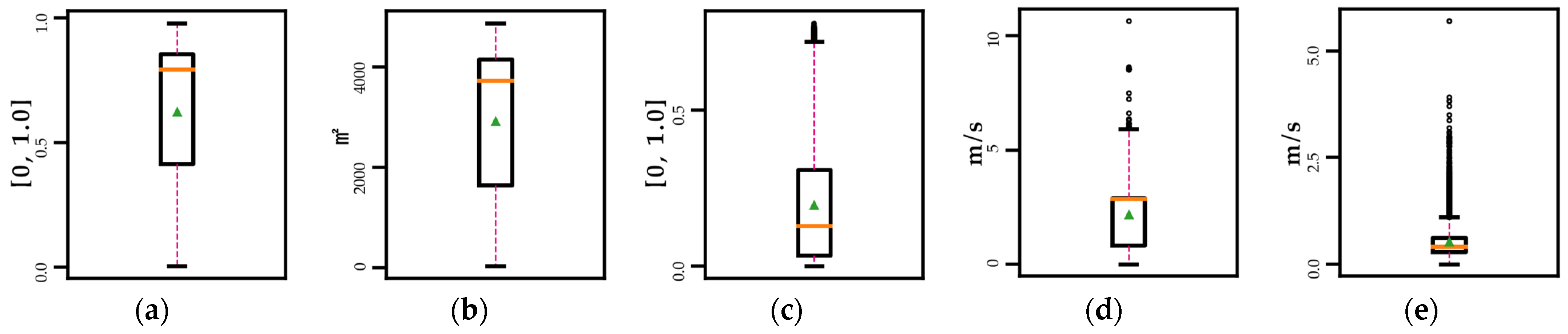
Water 16 00058 g015
Figure 16. Box plot of the dataset before data preprocessing. (a) Ice concentration. (b) Ice area. (c) Ice motion intensity. (d) Ice maximum velocity. We found abnormal values greater than 10 m/s. (e) The ice average velocity. We found abnormal values greater than 5 m/s.
Water 16 00058 g016
Figure 17. Box plot of the dataset after data preprocessing, with the modified abnormal values and the ice area and velocity normalized to [0, 1]. (a) Ice concentration. (b) Ice area. (c) Ice motion intensity. (d) Ice maximum velocity. (e) Ice average velocity.
Water 16 00058 g017
Figure 18. Training log curve. Accuracy and loss on the training set and validation set, respectively.
Water 16 00058 g018
Figure 19. Loss curve on the validation set with the different learning rates. A larger learning rate converged faster but was unstable, while a smaller one converged slower but was stable. Both the 0.01 and 0.1 learning rates ultimately achieved the highest accuracy of 0.9990 on the validation set.
Water 16 00058 g019
Figure 20. Real-time monitoring of the river ice regime in each break-up stage. The images were captured from the tenth-second frame of the corresponding video clip. The blue color represents the medium warning level; the red color represents the high warning level; the green color represents the low warning level; the grey color represents the none warning level.
Water 16 00058 g020
Table 1. The number of images in each stage.
No.The Stage of Ice Break-UpThe Number of VideosThe Number of IMAGES
1ice frozen1600
2ice break-up beginning63600
3ice drifting1060,000
4ice break-up ending63600
5ice-free31800
Total2615,600
Table 2. Comparison of the different methods on the IPC_RI_IDS dataset.
MethodsmIoUAccTime
FastScnn [23]0.96870.9821112 ms
MobileSeg [24]0.96660.9810115 ms
PPLiteSeg [25]0.96720.9813121 ms
PPMobileSeg [26]0.97620.9865121 ms
Table 3. Partial data for the ice regime parameters in the IPC_RI_IDS dataset.
No.StageIce ConcentrationIce AreaMotion IntensityMaximum VelocityAverage Velocity
210.97614857.95700.01000.00.0
410.97604857.31600.00500.00.0
510.97754865.07300.02000.00.0
610.97644860.01200.00500.00.0
1
303720.87054264.36500.04000.39040.1946
304020.86984259.46200.03500.38840.0971
304120.87074263.42600.04000.41360.2005
304220.87074264.11700.03500.41360.2010
612130.81713857.97600.48002.84090.4689
612230.81653854.65800.47503.32660.5130
612430.81593850.74200.48002.98830.2939
612530.81653854.58100.48002.86760.4193
10,53140.41621655.64500.05501.27550.4717
10,53340.41501652.17800.04501.20760.3242
10,53640.41361638.56000.04002.86781.1598
10,53740.41401645.85300.04002.95360.5697
14,54750.007451.81800.01000.45640.4551
14,54850.006243.31050.00500.45640.2282
14,54950.007149.85680.01500.90770.6820
14,55050.008559.50840.03000.00.0
Note: 1 Omit data.
Table 4. Comparison results of the three methods.
MethodsKernelAccuracyLoss
Softmax regression-0.90080.2782
SVMLinear0.8967-
Poly (degree = 5)0.9646-
RBF0.9190-
Sigmoid0.2684-
Ours-0.98130.0173
Table 5. River ice-related risk warning level of the five stages.
No.The Stage of Ice Break-UpWarning LevelNote
1Ice frozenMediumObserve if there is an ice jam
2Ice break-up beginningHighIce run is about to occur
3Ice driftingHighPay attention to blockage and collisions
4Ice break-up endingLowThe risk is minimal
5Ice-freeNoneThe river has been opened
Disclaimer/Publisher’s Note: The statements, opinions and data contained in all publications are solely those of the individual author(s) and contributor(s) and not of MDPI and/or the editor(s). MDPI and/or the editor(s) disclaim responsibility for any injury to people or property resulting from any ideas, methods, instructions or products referred to in the content.

