
A Hybrid Model for Water Quality Prediction Based on an Artificial Neural Network, Wavelet Transform, and Long Short-Term Memory


Abstract
:1. Introduction
2. Materials and Methods
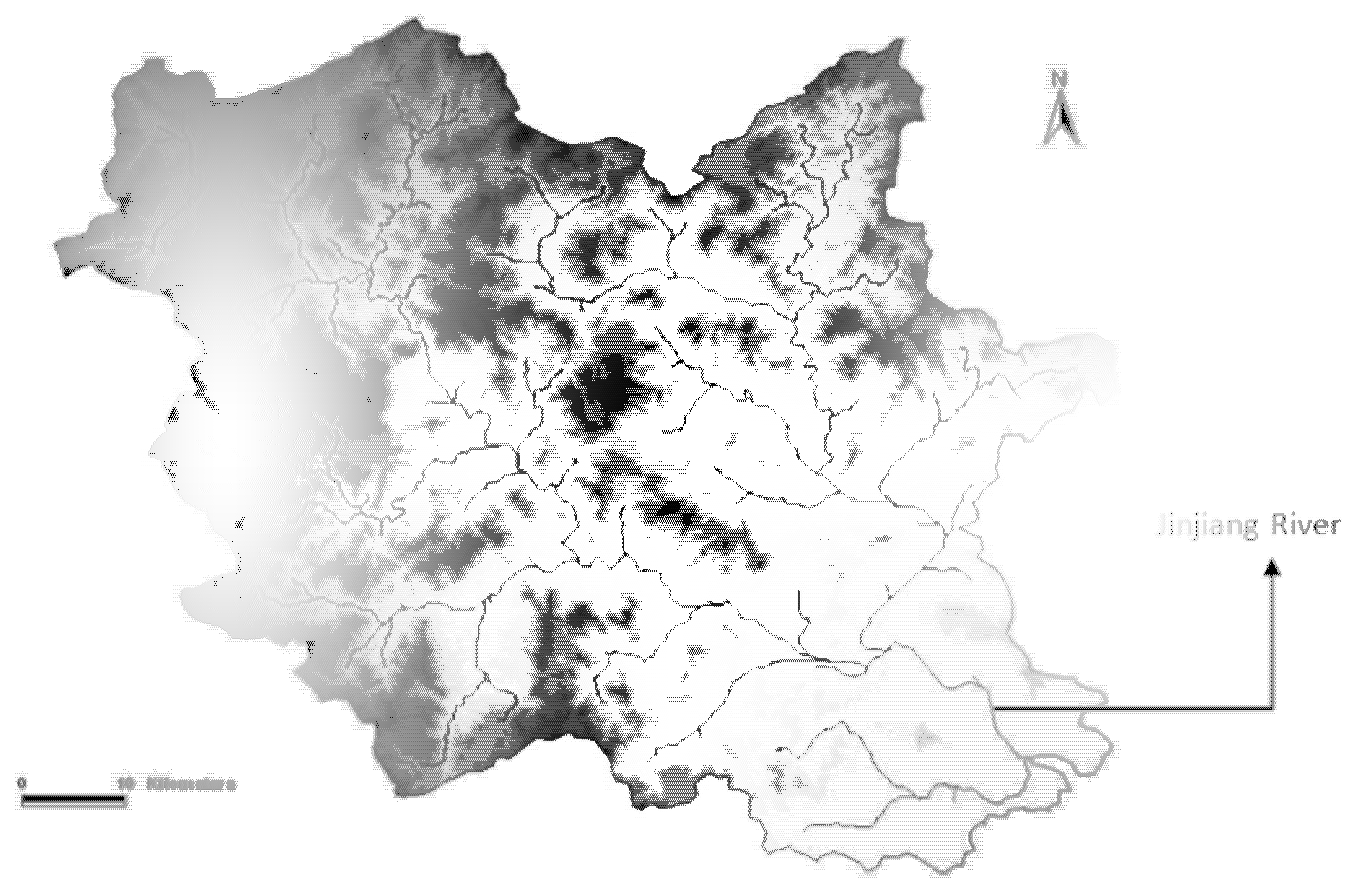
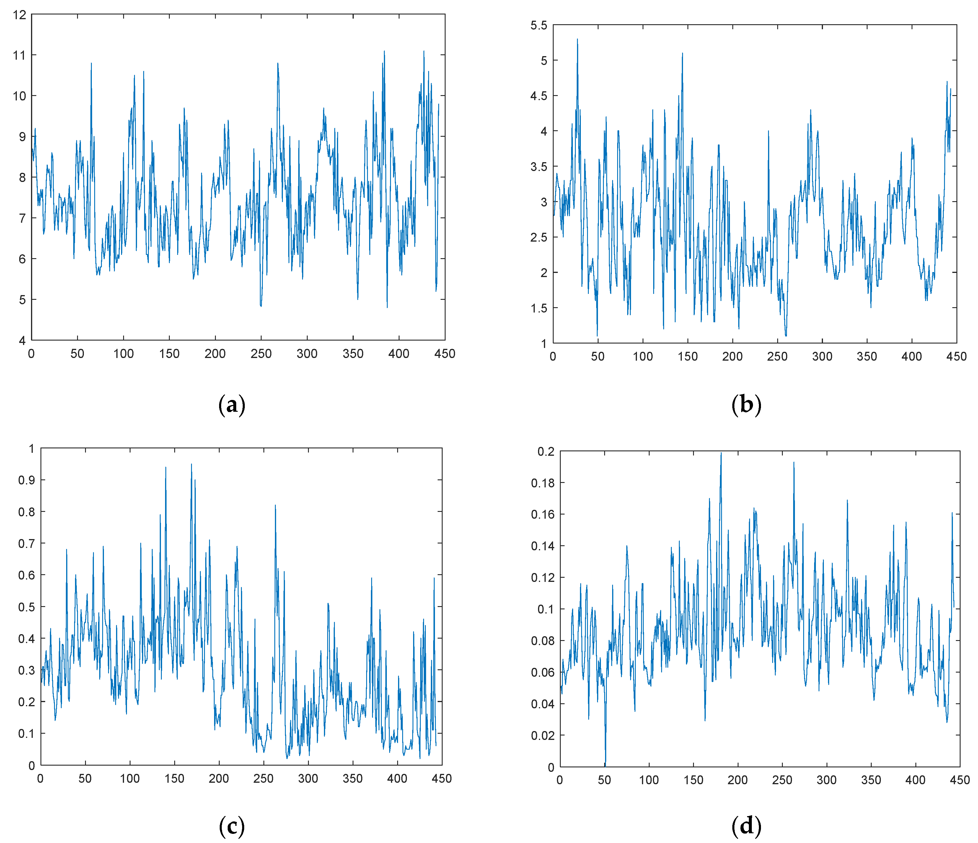
2.1. Study Area Description and Dataset Analysis
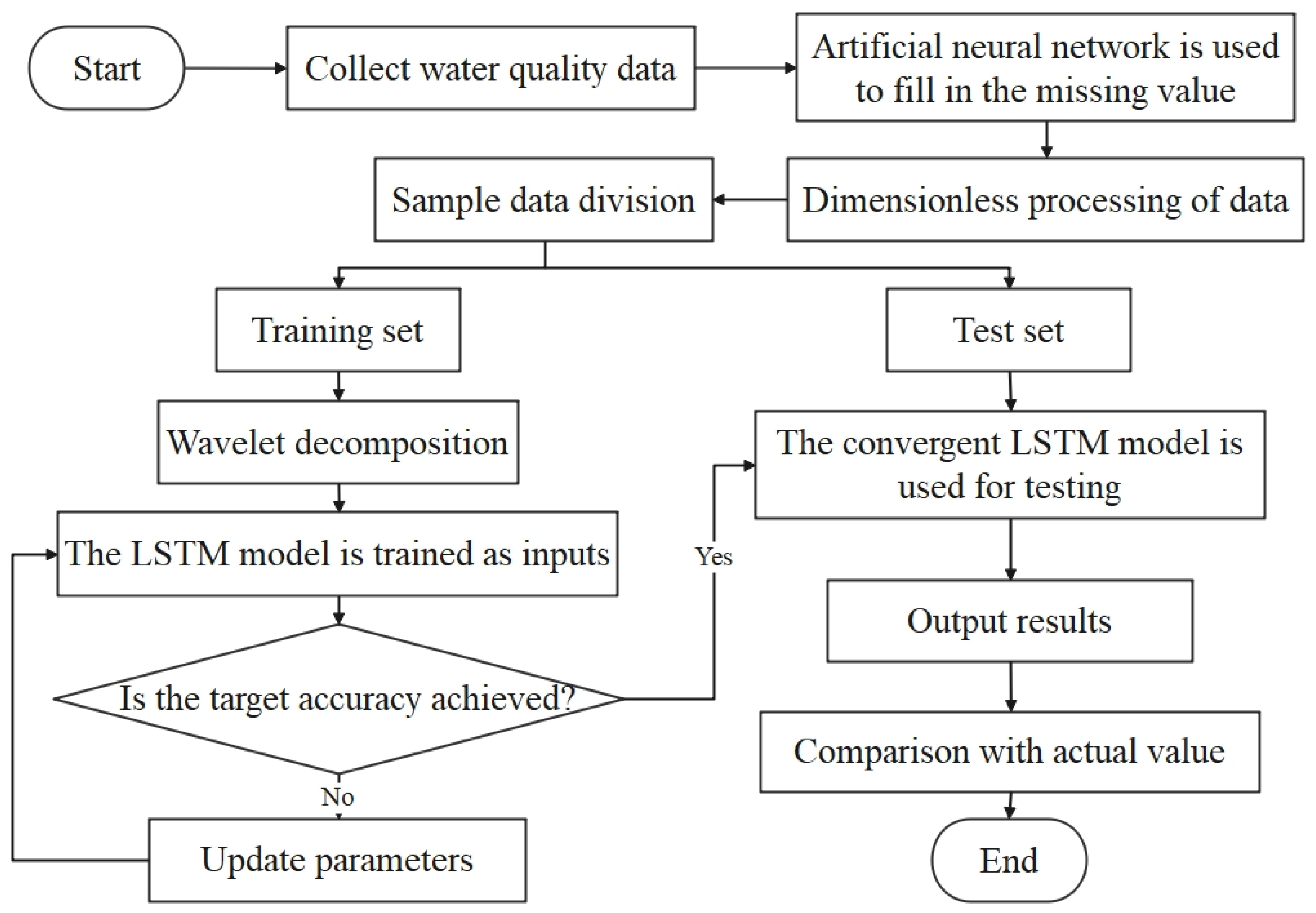
2.2. The Framework of the Proposed Model
- Data preprocessing: firstly make a descriptive analysis of the collected water quality data, find the missing value, estimate the missing value by artificial neural network, and then normalize it to eliminate the influence of dimension.
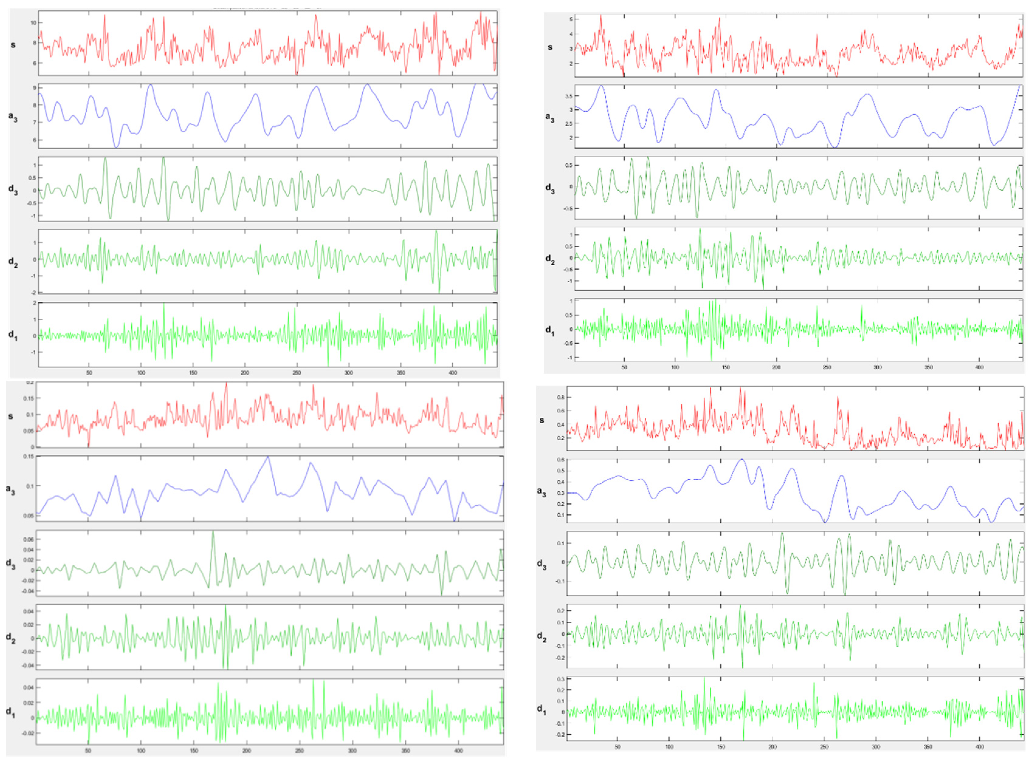
- Discrete wavelet transform: The db5 wavelet technique is used to decompose the water quality time series datasets.
- Model training, detection: Split the high-frequency and low-frequency signals of each dataset obtained from the db5 wavelet decomposition into a training set and a test set according to a fixed ratio. In this study, we set the first 421 sets of each dataset as the training set and the last 22 sets as the test set. Subsequently, we used LSTM to train each training set and adjust the relevant parameters of LSTM, such as learning rate and the maximum number of iterations.
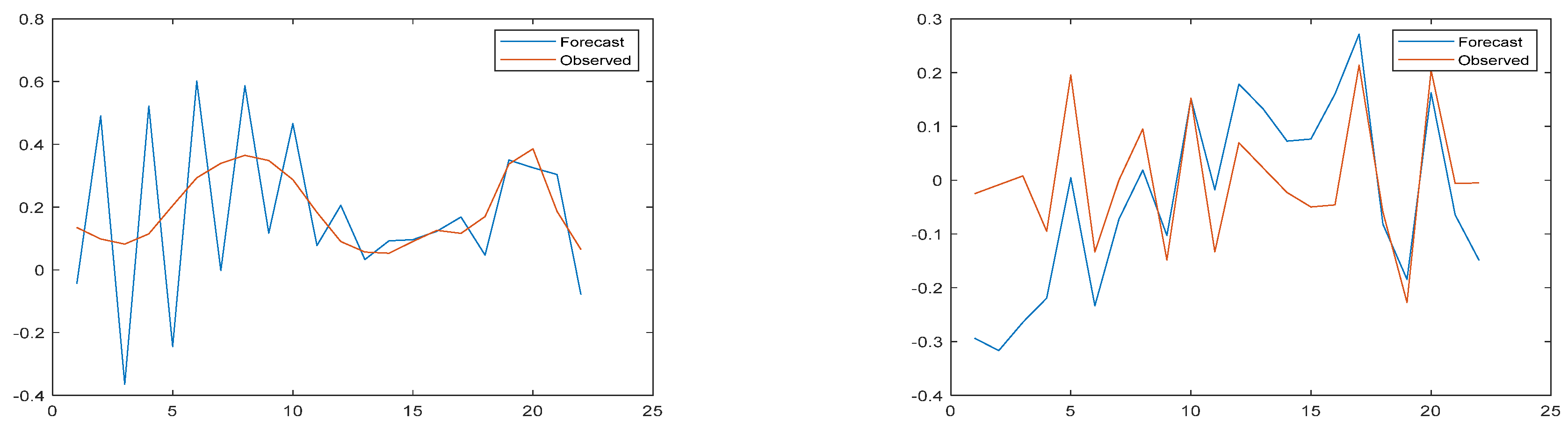
- The predictions obtained from the decomposed test set of each sub-series are superimposed to obtain the final prediction results.
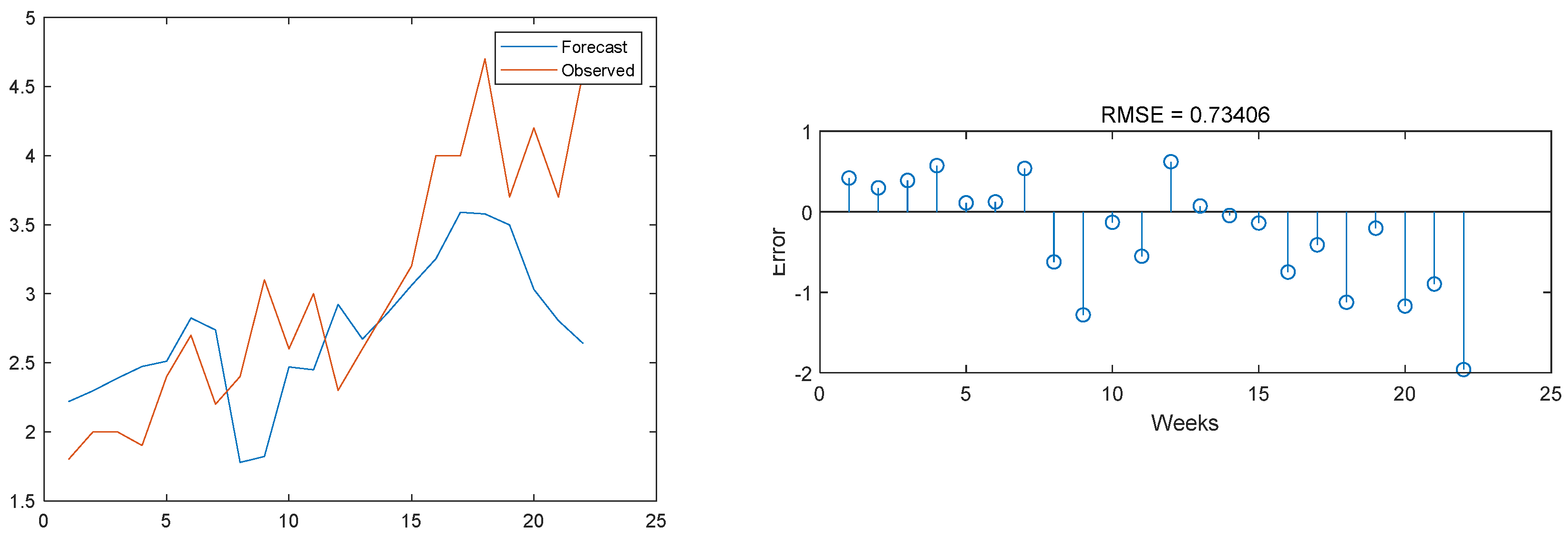
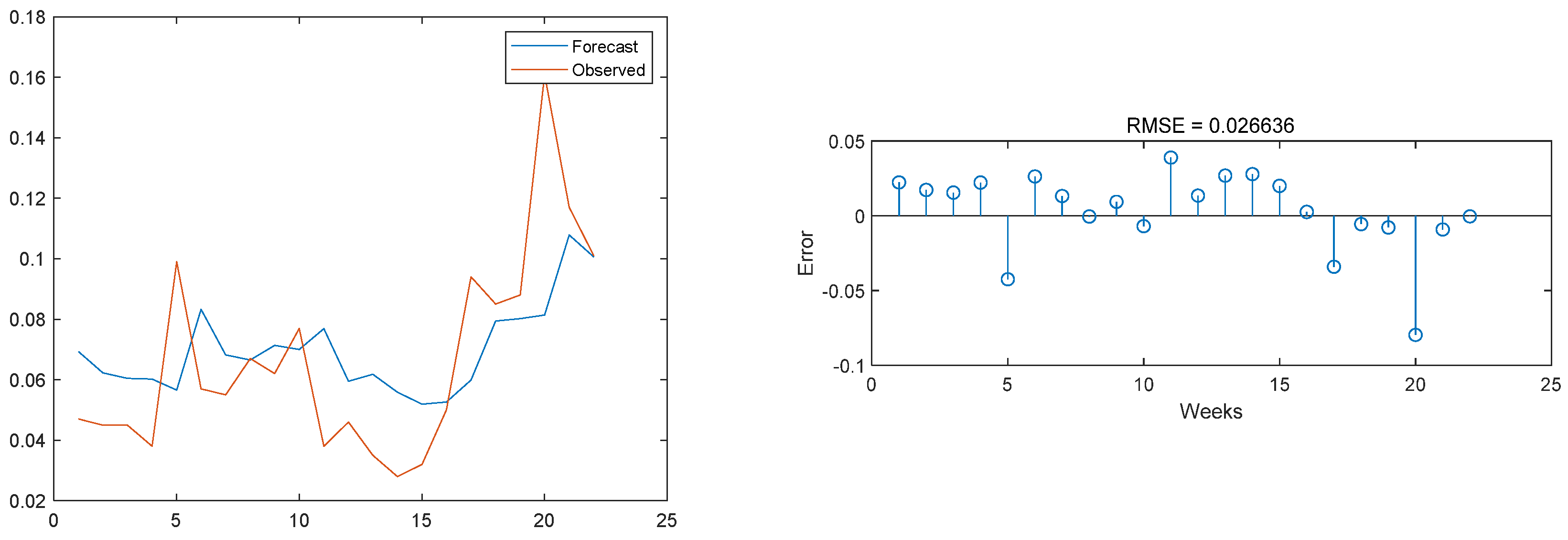
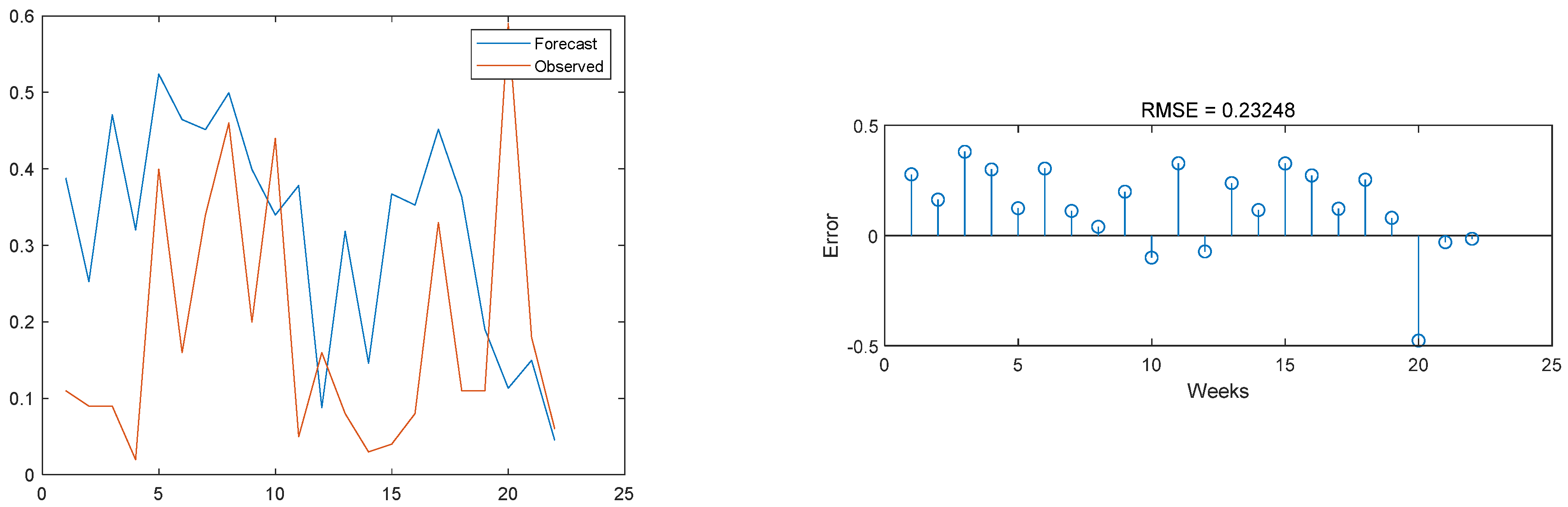
- Model evaluation: This study used four indicators—MSE, RMSE, MAE and MAPE—to evaluate the model’s performance.
2.3. Data Normalization
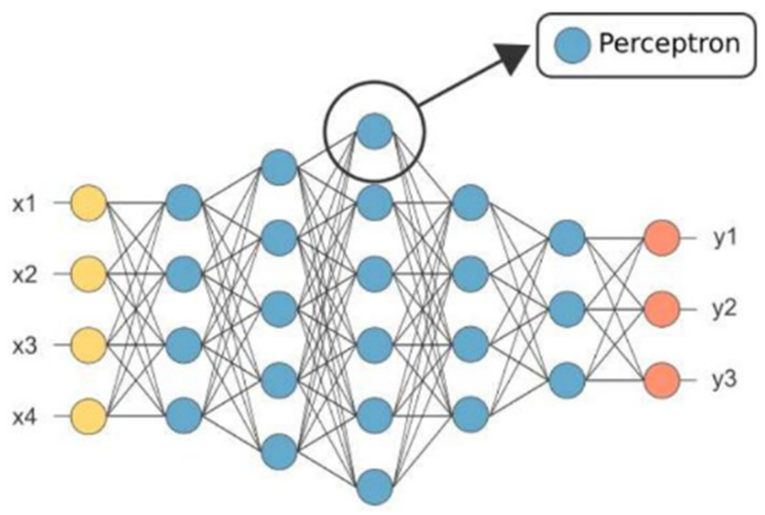
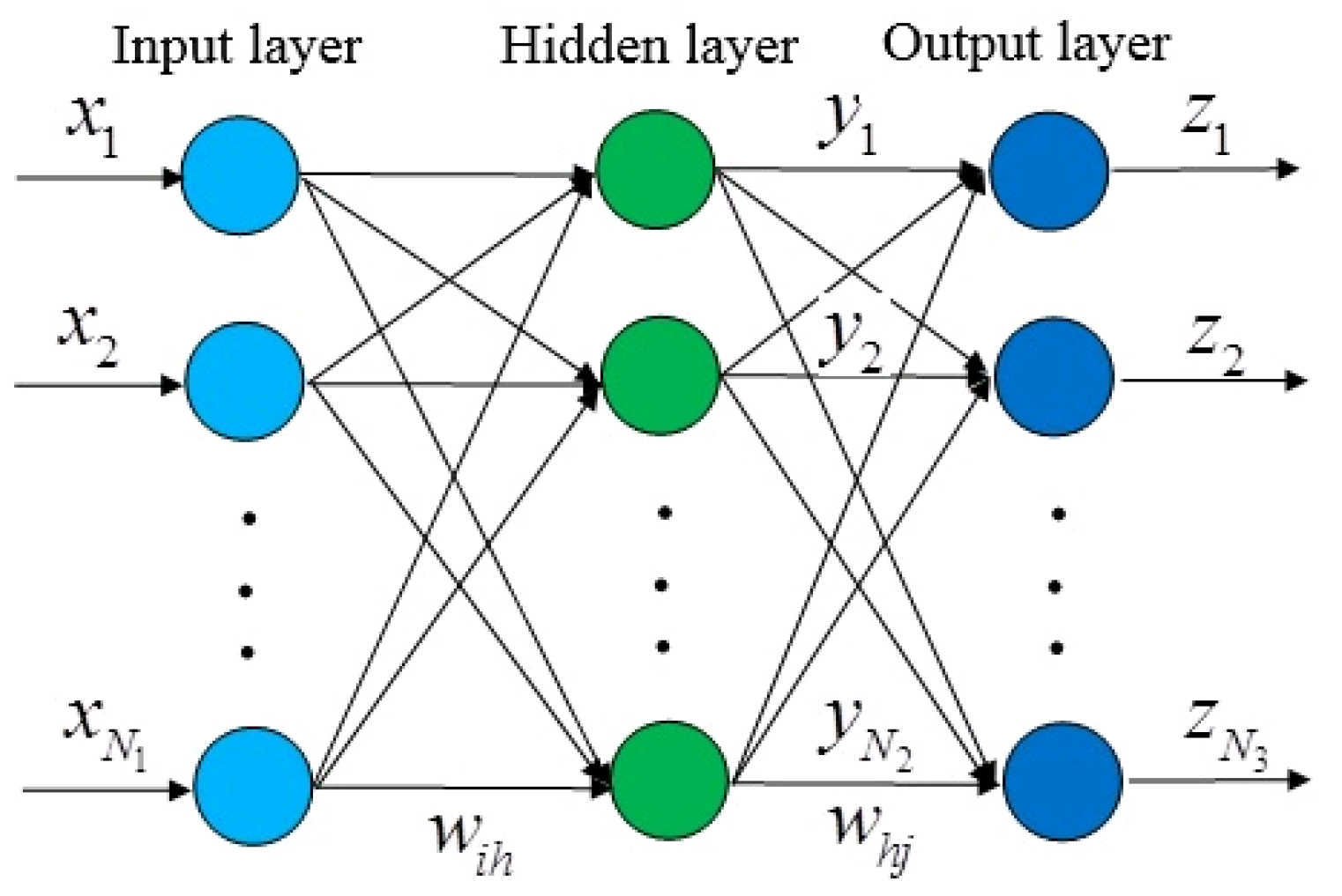
2.4. Artificial Neural Network (ANN)
2.5. Basic Principle of Wavelet Transform
- (1)
- The db wavelets are more suitable for relatively stable sequences;
- (2)
- db5 is also one of the most commonly used wavelets in the db wavelet family, which is suitable for smoother datasets.
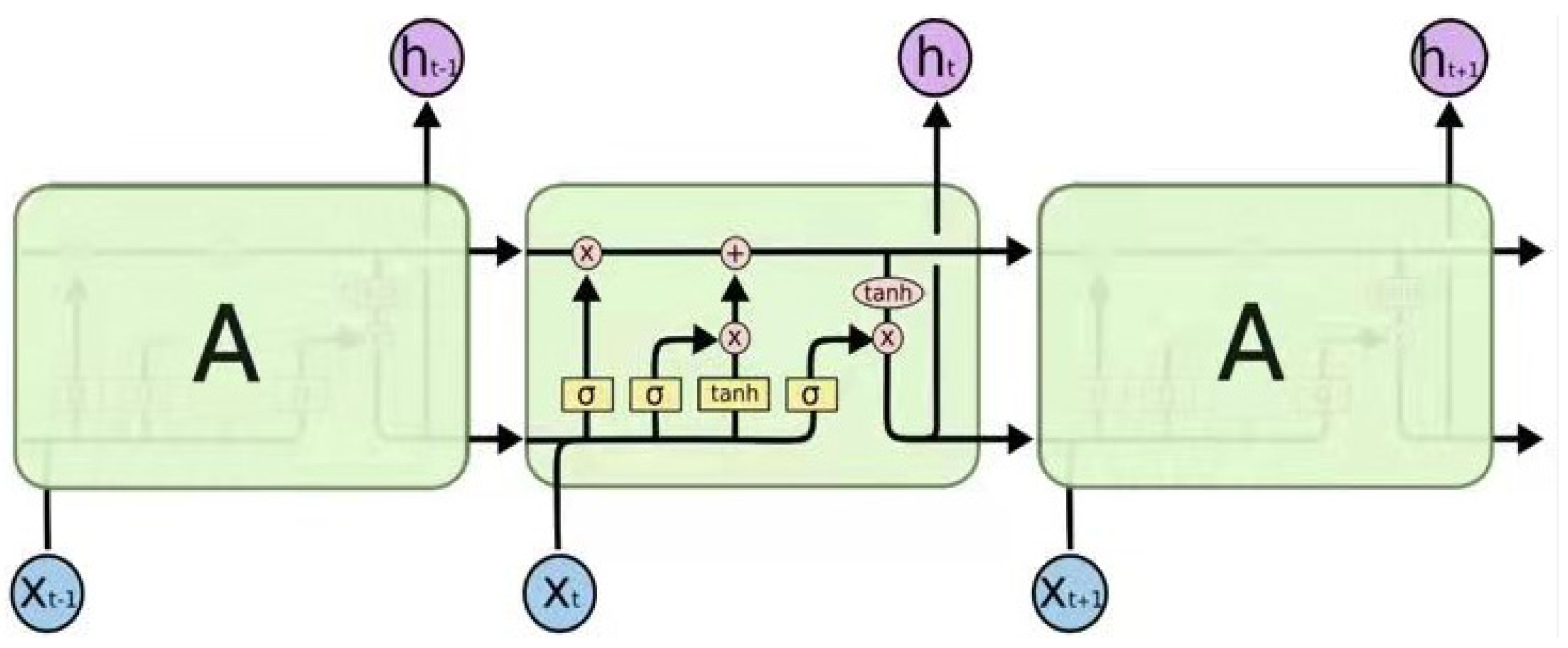
2.6. Basic Principle of LSTM
2.7. Evaluation Index
3. Results
3.1. Artificial Neural Network Interpolation
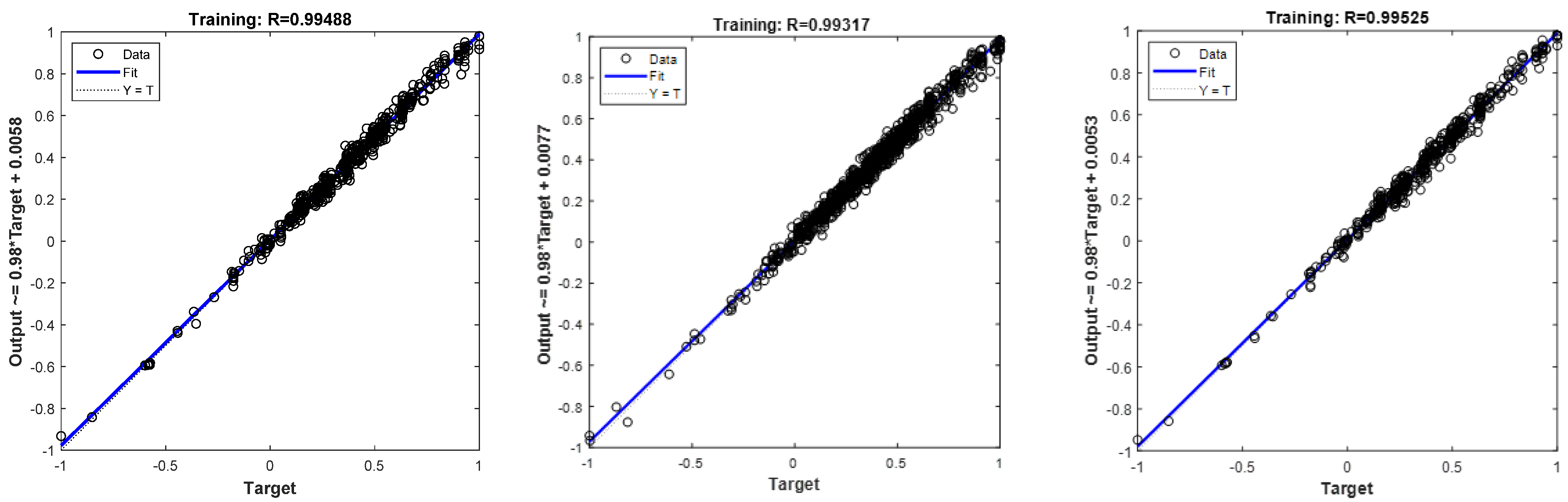
3.2. Results of Wavelet Transform Model
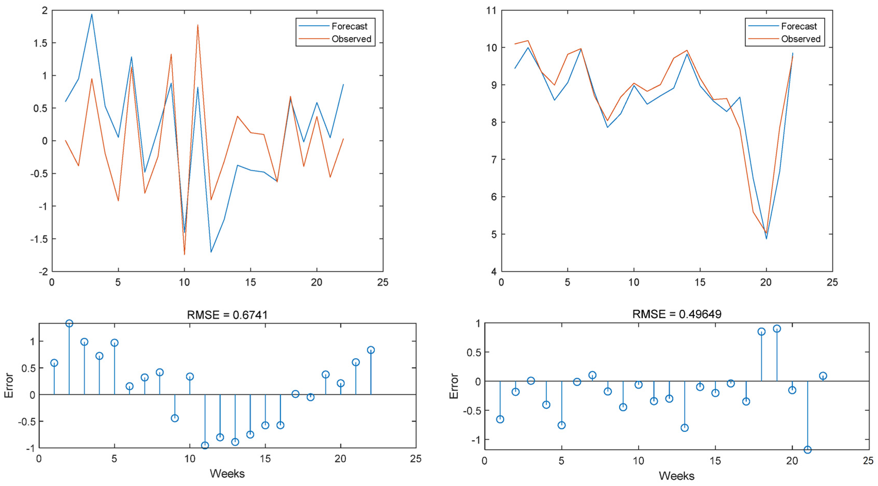
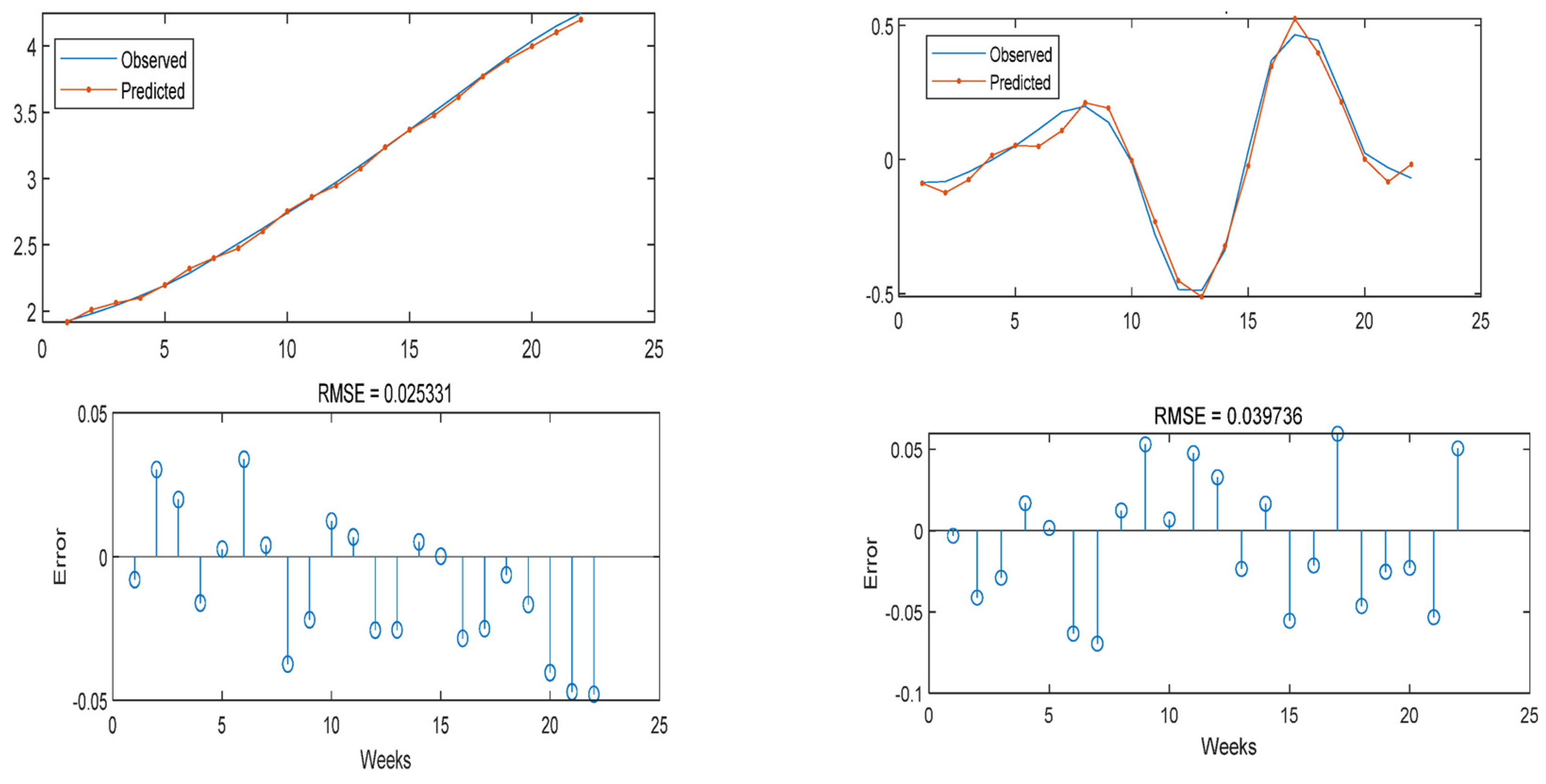
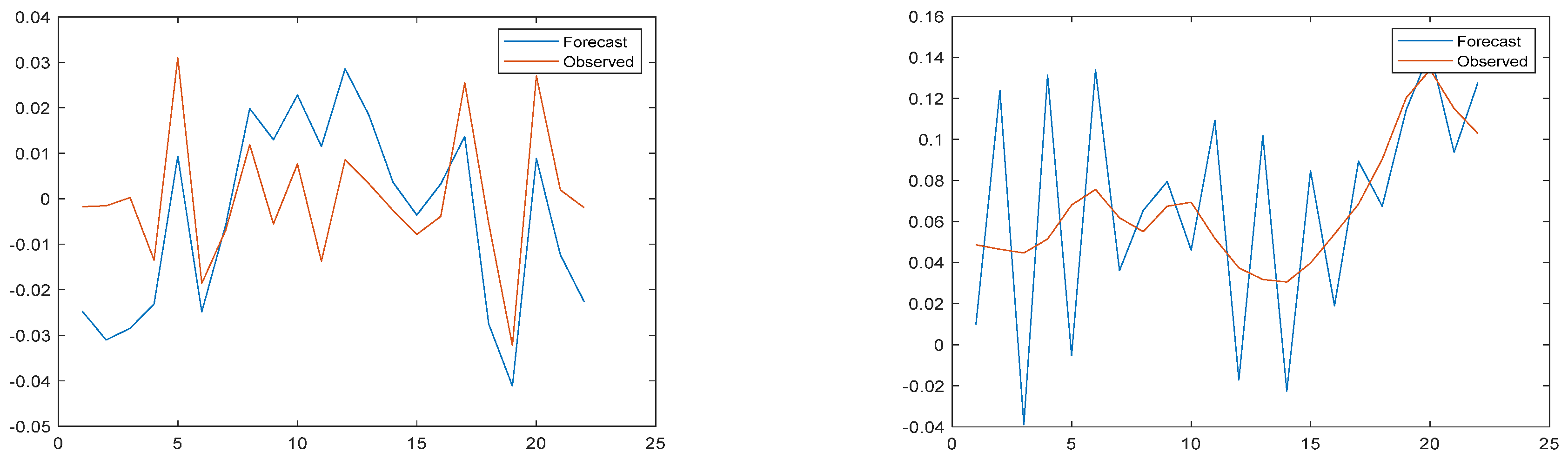
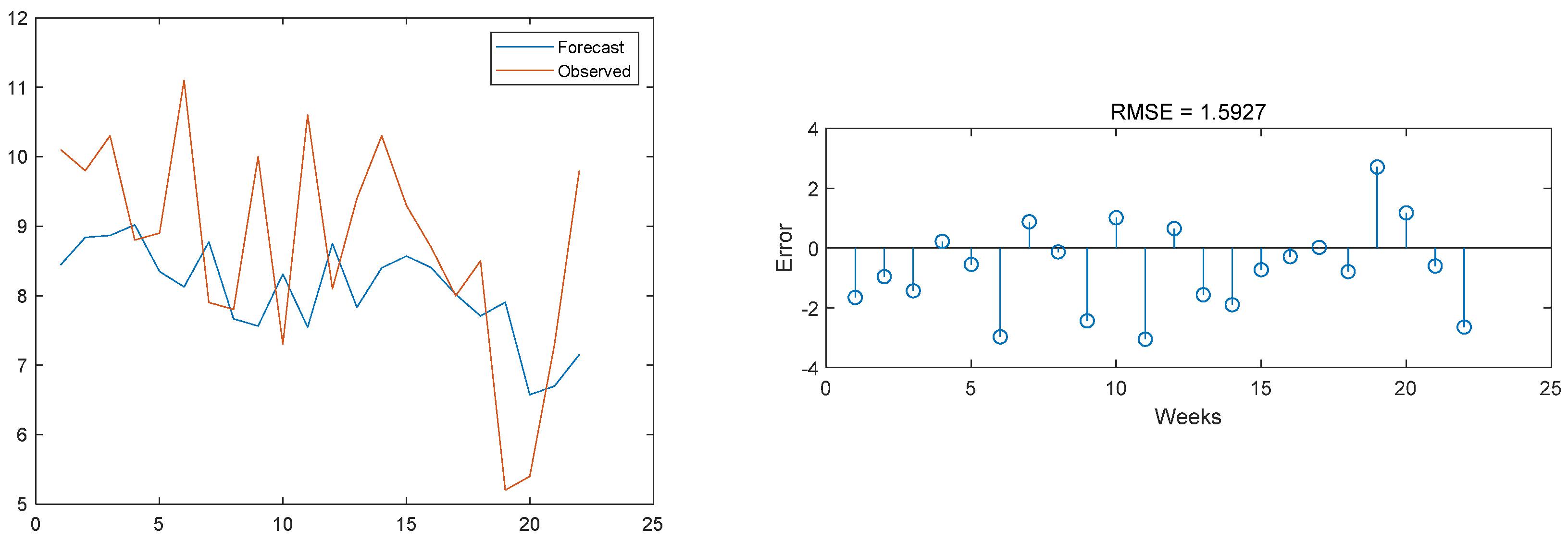
3.3. Model Result Output
3.4. Comparison with Other Models
4. Discussion
- (1)
- Existing monitoring systems cannot achieve online high-frequency monitoring of all important pollutants, so the model proposed in this study can be used for soft computing to improve the timeliness, coverage and frequency of online monitoring and to form an effective early warning system for water quality management.
- (2)
- According to real-time monitoring data for water quality change trend prediction and water quality risk judgment. When the prediction results show that the water quality situation has a deteriorating trend, the relevant management departments can make the corresponding measures of pollution prevention and control at the first time, so as to minimize the water quality losses caused by pollution incidents.
- (1)
- The model proposed in this paper only considers the historical data of water quality indicators in the Jinjiang River basin, while changes in the external environment have a greater impact on river water quality, which can interfere with the neural network training process, thus affecting the accuracy of the model. There is still room for further research into how to reduce the interference of external factors or consider the influence of water quality factors in the model.
- (2)
- In this study, LSTM was used to predict water quality; however, there are numerous improved versions of the LSTM model, including the Bi-LSTM (bi-directional long short-term memory network) and the adaptive neuro-fuzzy inference system (ANFIS). These methods can be used to compare with the model proposed in this study.
5. Conclusions
Author Contributions
Funding
Institutional Review Board Statement
Informed Consent Statement
Data Availability Statement
Acknowledgments
Conflicts of Interest
References
- Wang, Q.; Hao, D.; Li, F.; Guan, X.; Chen, P. Development of a new framework to identify pathways from socioeconomic development to environmental pollution. J. Clean Prod. 2020, 253, 119962. [Google Scholar] [CrossRef]
- Ministry of Water Resources. Water Resources Assessment in China; Water and Hydropower Publishing: Beijing, China, 2018; pp. 154–196.
- Shi, X. The Safety of Drinking Water in China: Current Status and Future Prospects. China CDC Wkly. 2020, 2, 210–215. [Google Scholar] [CrossRef] [PubMed]
- Hara, J.; Mamun, M.; An, K. Ecological river health assessments using chemical parameter model and the index of biological integrity model. Water 2019, 11, 1729. [Google Scholar] [CrossRef] [Green Version]
- Chen, X.; Strokal, M.; Van, V.; Michelle, T.; Stuiver, J.; Wang, M.; Bai, Z.; Kroeze, C.; Ma, L. Multi-scale Modeling of Nutrient Pollution in the Rivers of China. Environ. Sci. Technol. 2019, 53, 9614–9625. [Google Scholar] [CrossRef] [PubMed] [Green Version]
- Huang, J.; Zhang, Y.; Bing, H.; Peng, J.; Arhonditsis, G. Characterizing the river water quality in china: Recent progress and on-going challenges. Water Res. 2021, 201, 117309. [Google Scholar] [CrossRef] [PubMed]
- Sarpong, K.; Xu, W.; Mensah-Akoto, J.; Neequaye, J.; Dadzie, A.; Frimpong, O. Waterscape, State and Situation of China’s Water Resources. J. Geosci. Environ. Prot. 2020, 8, 26–51. [Google Scholar] [CrossRef]
- O’Connor, D. Oxygen Balance of an Estuary. Tran. Am. Soc. Civ. Eng. 1961, 126, 556–575. [Google Scholar] [CrossRef]
- Thomann, R. Mathematical Model for Dissolved Oxygen. J. Sanit. Eng. Div. 1963, 89, 1–32. [Google Scholar] [CrossRef]
- Dobbins, W. BOD and Oxygen Relationship in Streams. J. Sani. Eng. Div. 1964, 90, 53–78. [Google Scholar] [CrossRef]
- Ma, W.; Chao, Z. The numerical simulation of water quality of Suzhou Creek based on GIS. Acta Geogr. Sin. 1998, 53, 66–75. [Google Scholar]
- Zhang, Y.; Xia, J.; Shao, Q.; Zhai, X. Water quantity and quality simulation by improved SWAT in highly regulated Huai River Basin of China. Stoch. Env. Res. Risk Assess. 2013, 27, 11–27. [Google Scholar] [CrossRef]
- Peng, S.; Fu, G.; Zhao, X.; Moore, B. Integration of Environmental Fluid Dynamics Code (EFDC) Model with Geographical Information System (GIS) Platform and Its Applications. J. Environ. Inform. 2011, 17, 75–82. [Google Scholar] [CrossRef]
- Huang, M.; Tian, Y. An Integrated Graphic Modeling System for Three-Dimensional Hydrodynamic and Water Quality Simulation in Lakes. ISPRS Int. J. Geo-Inf. 2019, 8, 18. [Google Scholar] [CrossRef] [Green Version]
- Lee, I.; Hwang, H.; Lee, J.; Yu, N.; Yun, J.; Kim, H. Modeling approach to evaluation of environmental impacts on river water quality: A case study with Galing River, Kuantan, Pahang, Malaysia. Ecol. Model. 2017, 353, 167–173. [Google Scholar] [CrossRef]
- Deus, R.; Brito, D.; Mateus, M.; Kenov, I.; Fornaro, A.; Neves, R.; Alves, C. Impact evaluation of a pisciculture in the Tucuruí reservoir (Pará, Brazil) using a two-dimensional water quality model. J. Hydrol. 2013, 487, 1–12. [Google Scholar] [CrossRef]
- Al-Zubaidi, H.A.M.; Wells, S.A. Analytical and field verification of a 3D hydrodynamic and water quality numerical scheme based on the 2D formulation in CE-QUAL-W2. J. Hydraul. Res. 2018, 58, 152–171. [Google Scholar] [CrossRef] [Green Version]
- Yang, L.K.; Peng, S.; Zhao, X.H.; Li, X. Development of a two-dimensional eutrophication model in an urban lake (China) and the application of uncertainty analysis. Ecol. Model. 2017, 345, 63–74. [Google Scholar]
- Colton, B.; Tassiane, J.; Alice, D.; Bas, V. Mass-Balance Modeling of Metal Loading Rates in the Great Lakes. Environ. Res. 2022, 205, 112557. [Google Scholar]
- Wang, X.; Jia, J.; Su, T.; Zhao, Z.; Xu, J.; Li, W. A fusion water quality soft-sensing method based on wasp model and its application in water eutrophication evaluation. J. Chem. 2018, 2018, 9616841. [Google Scholar] [CrossRef] [Green Version]
- Yang, H.; Wang, J.; Li, J.; Zhou, H.; Liu, Z. Modelling impacts of water diversion on water quality in an urban artificial lake. Environ. Pollut. 2021, 276, 116694. [Google Scholar] [CrossRef]
- Najafzadeh, M.; Noori, R.; Afroozi, D.; Ghiasi, B.; Hosseini-Moghari, S.M.; Mirchi, A.; Haghighi, A.T.; Kløve, B. A comprehensive uncertainty analysis of model-estimated longitudinal and lateral dispersion coefficients in open channels. J. Hydrol. 2021, 603, 126850. [Google Scholar] [CrossRef]
- Song, C.; Yao, L.; Hua, C.; Ni, Q. A novel hybrid model for water quality prediction based on synchrosqueezed wavelet transform technique and improved long short-term memory. J. Hydrol. 2021, 603, 126879. [Google Scholar] [CrossRef]
- Noori, R.; Safavi, S.; Shahrokni, S.A.N. A reduced-order adaptive neuro-fuzzy inference system model as a software sensor for rapid estimation of five-day biochemical oxygen demand. J. Hydrol. 2013, 495, 175–185. [Google Scholar] [CrossRef]
- Noori, R.; Karbassi, A.R.; Ashrafi, K.; Ardestani, M.; Mehrdadi, N. Development and application of reduced-order neural network model based on proper orthogonal decomposition for BOD5 monitoring: Active and online prediction. Environ. Prog. Sustain. Energy 2013, 32, 120–127. [Google Scholar] [CrossRef]
- Noori, R.; Yeh, H.D.; Abbasi, M.; Kachoosangi, F.T.; Moazami, S. Uncertainty analysis of support vector machine for online prediction of five-day biochemical oxygen demand. J. Hydrol. 2015, 527, 833–843. [Google Scholar] [CrossRef]
- Ahmed, U.; Mumtaz, R.; Anwar, H.; Shah, A.; García-Nieto, J. Efficient Water Quality Prediction Using Supervised Machine Learning. Water 2019, 11, 2210. [Google Scholar] [CrossRef] [Green Version]
- Liu, P.; Wang, J.; Sangaiah, A.; Xie, Y.; Yin, X. Analysis and Prediction of Water Quality Using LSTM Deep Neural Networks in IoT Environment. Sustainability 2019, 11, 2058. [Google Scholar] [CrossRef] [Green Version]
- Hu, Z.; Zhang, Y.; Zhao, Y.; Xie, M.; Zhong, J.; Tu, Z.; Liu, J. A water quality prediction method based on the deep LSTM network considering correlation in smart mariculture. Sensors 2019, 19, 1420. [Google Scholar] [CrossRef] [Green Version]
- Eze, E.; Halse, S.; Ajmal, T. Developing a Novel Water Quality Prediction Model for a South African Aquaculture Farm. Water 2021, 13, 1782. [Google Scholar] [CrossRef]
- Solanki, A.; Agrawal, H.; Khare, K. Predictive Analysis of Water Quality Parameters using Deep Learning. Int. J. Comput. Appl. 2015, 125, 29–34. [Google Scholar] [CrossRef] [Green Version]
- Wang, J.; Zhang, L.; Zhang, W.; Wang, X. Reliable Model of Reservoir Water Quality Prediction Based on Improved ARIMA Method. Environ. Eng. Sci. 2019, 36, 1041–1048. [Google Scholar] [CrossRef]
- Abdel-Fattah, M.; Mokhtar, A.; Abdo, A. Application of neural network and time series modeling to study the suitability of drain water quality for irrigation: A case study from Egypt. Environ. Sci. Pollut. R. 2021, 28, 898–914. [Google Scholar] [CrossRef] [PubMed]
- Shi, B.; Peng, W.; Jiang, J.; Liu, R. Applying high-frequency surrogate measurements and a wavelet-ANN model to provide early warnings of rapid surface water quality anomalies. Sci. Total Environ. 2018, 1390, 610–611. [Google Scholar] [CrossRef] [PubMed]
- Li, X.; Cheng, Z.; Yu, Q.; Bai, Y.; Li, C. Water-Quality Prediction Using Multimodal Support Vector Regression: Case Study of Jialing River, China. J. Environ. Eng. 2017, 143, 4017070. [Google Scholar] [CrossRef]
- Ewaid, S.; Abed, S.; Kadhum, S. Prediction the Tigris river water quality within Baghdad, Iraq by using water quality index and regression analysis. Environ. Technol. Innov. 2018, 11, 390–398. [Google Scholar] [CrossRef]
- Xu, L.; Liu, S. Study of short-term water quality prediction model based on wavelet neural network. Mat. Comput. Model. 2013, 58, 801–807. [Google Scholar] [CrossRef]
- Long, S. Study of Short-term Water Quality Prediction Model Based on PSO-WSVR. J. Zhengzhou Univ. 2013, 58, 807–813. [Google Scholar]
- Tizro, A.; Ghashghaie, M.; Georgiou, P.; Voudouris, K. Time series analysis of water quality parameters. J. Appl. Res. Water Wastewater 2014, 1, 43–52. [Google Scholar]
- Faruk, D. A hybrid neural network and ARIMA model for water quality time series prediction. Eng. Appl. Artif. Intel. 2010, 23, 586–594. [Google Scholar] [CrossRef]
- Zhang, L.; Zhang, G.; Li, R. Water Quality Analysis and Prediction Using Hybrid Time Series and Neural Network Models. J. Agric. Sci. Tech. IRAN 2016, 18, 975–983. [Google Scholar]
- Than, N.; Ly, C.; Tat, P. The performance of classification and forecasting Dong Nai River water quality for sustainable water resources management using neural network techniques. J. Hydrol. 2021, 596, 126099. [Google Scholar] [CrossRef]
- Zhou, J.; Wang, Y.; Xiao, F.; Wang, Y.; Sun, L. Water Quality Prediction Method Based on IGRA and LSTM. Water 2018, 10, 1148. [Google Scholar] [CrossRef] [Green Version]
- Hameed, M.; Sharqi, S.; Yaseen, Z.; Afan, H.; Hussain, A.; Elshafie, A. Application of artificial intelligence (AI) techniques in water quality index prediction: A case study in tropical region, Malaysia. Neural Comput. Appl. 2017, 28, 893–905. [Google Scholar] [CrossRef]
- Deng, J.; Guo, P.; Zhang, X.; Shen, X.; Su, H.; Zhang, Y.; Wu, Y.; Xu, C. An evaluation on the bioavailability of heavy metals in the sediments from a restored mangrove forest in the Jinjiang Estuary, Fujian, China. Ecotox. Environ. Safe. 2019, 180, 501–508. [Google Scholar] [CrossRef] [PubMed]
- Liu, X.; Jiang, J.; Yan, Y.; Dai, Y.; Deng, B.; Ding, S.; Su, S.; Sun, W.; Li, Z.; Gan, Z. Distribution and risk assessment of metals in water, sediments, and wild fish from Jinjiang River in Chengdu, China. Chemosphere 2018, 196, 45–52. [Google Scholar] [CrossRef]
- Chen, P. Effects of normalization on the entropy-based TOPSIS method. Expert Syst. Appl. 2019, 136, 33–41. [Google Scholar] [CrossRef]
- Alkhodari, M.; Fraiwan, L. Convolutional and recurrent neural networks for the detection of valvular heart diseases in phonocardiogram recordings. Comput. Methods Prog. Bio. 2021, 200, 105940. [Google Scholar] [CrossRef]
- Newman, D. Missing data: Five practical guidelines. Organ. Res. Methods 2014, 17, 372–411. [Google Scholar] [CrossRef]
- Little, R.; Rubin, D. Statistical Analysis with Missing Data, 2nd ed.; John Wiley & Sons: Hoboken, NJ, USA, 2014. [Google Scholar]
- Little, R.; Rubin, D. The analysis of social science data with missing values. Sociol. Method Res. 1989, 18, 292–326. [Google Scholar] [CrossRef]
- Shan, Y.; Deng, G. Kernel PCA regression for missing data estimation in DNA microarray analysis. In Proceedings of the 2009 IEEE International Symposium on Circuits and Systems, Taipei, Taiwan, 24–27 May 2009; pp. 1477–1480. [Google Scholar]
- Wang, Z.; Wu, X.; Wang, H.; Wu, T. Prediction and analysis of domestic water consumption based on optimized grey and Markov model. Water Supply 2021, 21, 3887–3899. [Google Scholar] [CrossRef]
- Wu, J.; Wang, Z.; Dong, L. Prediction and analysis of water resources demand in Taiyuan City based on principal component analysis and BP neural network. J. Water Supply Res. Tech. 2021, 70, 1272–1286. [Google Scholar] [CrossRef]
- Wu, X.; Wang, Z.; Wu, T.; Bao, X. Solving the Family Traveling Salesperson Problem in the Adleman-Lipton model based on DNA computing. IEEE Trans. Nanobiosci. 2022, 21, 75–85. [Google Scholar] [CrossRef] [PubMed]
- Noori, R.; Karbassi, A.R.; Mehdizadeh, H.; Vesali-Naseh, M.; Sabahi, M.S. A framework development for predicting the longitudinal dispersion coefficient in natural streams using an artificial neural network. Environ. Prog. Sustain. 2011, 30, 439–449. [Google Scholar] [CrossRef]
- Wang, Z.; Bao, X.; Wu, T. A Parallel Bioinspired Algorithm for Chinese Postman Problem Based on Molecular Computing. Comput. Intel. Neurosc. 2021, 2021, 8814947. [Google Scholar] [CrossRef]
- Austin, C.; White, R.; Buuren, V. Missing Data in Clinical Research: A Tutorial on Multiple Imputation. Can. J. Cardiol. 2020, 37, 1322–1331. [Google Scholar] [CrossRef] [PubMed]
- Chang, C.; Deng, Y.; Jiang, X.; Long, Q. Multiple imputation for analysis of incomplete data in distributed health data networks. Nat. Commun. 2020, 11, 5467. [Google Scholar] [CrossRef]
- Goudarzi, M.A.; Cocard, M.; Santerre, R.; Woldai, T. GPS interactive time series analysis software. GPS Solut. 2013, 17, 595–603. [Google Scholar] [CrossRef]
- Bao, Z.; Chang, G.; Zhang, L.; Chen, G.; Zhang, S. Filling missing values of multi-station GNSS coordinate time series based on matrix completion. Measurement 2021, 183, 109862. [Google Scholar] [CrossRef]
- Gia, B.; Te, A.; Bksa, C. Evaluating missing value imputation methods for food composition databases. Food Chem. Toxicol. 2020, 141, 111368. [Google Scholar]
- Tutz, G.; Ramzan, S. Improved methods for the imputation of missing data by nearest neighbor methods. Comput. Stat. Data Anal. 2015, 90, 84–99. [Google Scholar] [CrossRef] [Green Version]
- Deng, A.; Wang, Z.; Liu, H.; Wu, T. A bio-inspired algorithm for a classical water resources allocation problem based on Adleman-Lipton model. Desalin. Water Treat. 2020, 185, 168–174. [Google Scholar] [CrossRef]
- Li, R.; Chang, Y.; Wang, Z. Study on optimal allocation of water resources in Dujiangyan irrigation district of China based on improved genetic algorithm. Water Supply 2021, 21, 2989–2999. [Google Scholar] [CrossRef]
- Ji, Z.; Wang, Z.; Deng, X.; Huang, W.; Wu, T. A new parallel algorithm to solve one classic water resources optimal allocation problem based on inspired computational model. Desalin. Water Treat. 2019, 160, 214–218. [Google Scholar] [CrossRef] [Green Version]
- Yu, M. Short-term wind speed forecasting based on random forest model combining ensemble empirical mode decomposition and improved harmony search algorithm. Int. J. Green Energy 2020, 17, 332–348. [Google Scholar] [CrossRef]
- Arvanaghi, R.; Danishvar, S.; Danishvar, M. Classification cardiac beats using arterial blood pressure signal based on discrete wavelet transform and deep convolutional neural network. Biomed. Signal. Proces. Control. 2022, 71, 103131. [Google Scholar] [CrossRef]
- Hochreiter, S.; Schmidhuber, J. Long short-term memory. Neural Comput. 1997, 9, 1735–1780. [Google Scholar] [CrossRef]
- Yan, S. Understanding LSTM and Its Diagrams. Available online: https://blog.mlreview.com/understanding-lstm-and-its-diagrams-37e2f46f1714 (accessed on 8 February 2021).
- Fang, Z.; Wang, Y.; Peng, L.; Hong, H. Predicting flood susceptibility using LSTM neural networks. J. Hydrol. 2020, 594, 125734. [Google Scholar] [CrossRef]
- Chen, Y.; Lin, M.; Yu, R.; Wang, T. Research on simulation and state prediction of nuclear power system based on LSTM neural network. Sci. Technol. Nucl. Ins. 2021, 2021, 8839867. [Google Scholar] [CrossRef]
- Rui, F.; Suzuki, H.; Kitajima, T.; Kuwahara, A.; Yasuno, T. Wind Speed Prediction Model Using LSTM and 1D-CNN. J. Signal. Process. 2018, 22, 207–210. [Google Scholar]
- Ehsan, M.; Shahirinia, A.; Zhang, N.; Oladunni, T. Wind Speed Prediction and Visualization Using Long Short-Term Memory Networks (LSTM). In Proceedings of the 10th International Conference on Information Science and Technology (ICIST), Bath/London/Plymouth, UK, 9–15 September 2020. [Google Scholar]
- Troiano, L.; Villa, E.; Loia, V. Replicating a Trading Strategy by Means of LSTM for Financial Industry Applications. IEEE T. Ind. Inform. 2018, 14, 3226–3234. [Google Scholar] [CrossRef]
- Sundermeyer, M.; Schlüter, R.; Ney, H. LSTM Neural Networks for Language Modeling. In Proceedings of the 13th Annual Conference of the International Speech Communication Association 2012 (INTERSPEECH 2012), Portland, OR, USA, 9–13 September 2012; pp. 194–197. [Google Scholar]
- Liao, Z.; Li, Y.; Xiong, W.; Wang, X.; Liu, D.; Zhang, Y.; Li, C. An in-depth assessment of water resource responses to regional development policies using hydrological variation analysis and system dynamics modeling. Sustainability 2020, 12, 5814. [Google Scholar] [CrossRef]
- Horn, A.L.; Rueda, F.J.; Hormann, G.; Fohrer, N. Implementing river water quality modelling issues in mesoscale watershed models for water policy demands--an overview on current concepts, deficits, and future tasks. Phys. Chem. Earth. 2004, 29, 725–737. [Google Scholar] [CrossRef]
- Li, X.; Huang, M.; Wang, R. Numerical simulation of Donghu Lake hydrodynamics and water quality based on remote sensing and MIKE 21. ISPRS Int. J. Geo-Inf. 2020, 9, 94. [Google Scholar] [CrossRef] [Green Version]


| Water Quality Mechanical Prediction Methods | |||
|---|---|---|---|
| Research Scholars | Research Subjects | Model Name | Model Characteristics |
| Lee et al. (2017) [15] | Environmental Fluid Dynamic Code | The Galing River in Kuantan, Pahang, Malaysia | The Environmental Fluid Dynamic Code (EFDC) model considers the effects of temperature, humidity, radiation, cloud cover, evaporation, wind direction, and wind speed, which makes the simulation results closer to the reality. The water quality (TOC, TN, TP) in the upstream section is significantly improved, and the prediction accuracy can be improved by about 37%; if the sewage from the tributary is at the same location, it will increase by about 77%. A total of five water quality management plans for improving the water quality of the Galing River were evaluated using EFDC. |
| Deus et al. (2013) [16] | Two-dimensional water quality model | The Tucuruí reservoir, Pará, Brazil | The use of CE-QUAL-W2 to model hydrodynamics and water quality can reproduce horizontal and vertical gradients and their temporal changes. The field data of temperature, nitrate, ammonia, phosphorus, total suspended solids (TSS), and dissolved oxygen and chlorophyll a are used to verify the prediction effect of the model, and it has been confirmed that it can be used to simulate the response of water quality to the various management schemes of the fish industry. |
| Al-Zubaidi and Wells (2018) [17] | Three-dimensional hydrodynamic model | Lake Chaplain, Washington, DC, USA | The 3D hydrodynamic and water quality model is developed by expanding the 2D fully implicit scheme of CE-QUAL-W2 in three dimensions. The governing equations include a continuity equation, free surface equation, momentum equation, and transport equation, and the momentum and transport equations are solved by the time-splitting technique. The hydrodynamic equation and water quality equation are solved at the same time to realize the feedback between water quality and hydrodynamics. The results showed that the solution of the hydrodynamic equation of the model was very consistent with the field data. |
| Yang et al. (2017) [18] | Finite volume method | Urban Lake in Tianjin, China | The Navier Stokes equation is used to establish a two-dimensional hydraulic model, the finite volume method is used to calculate the parameters of the two-dimensional uncertain eutrophication model, and the Bayesian method is used to correct the model parameters. The model reflects the interaction between nutrients, phytoplankton, and zooplankton. It can be used to simulate the changes of seasonal and regional water quality indicators (DO, NH4+, NO3−, and PO43−), and can calculate hydrodynamic information and eutrophication dynamics with reasonable accuracy (all relative errors are less than 11%). |
| Colton et al. (2022) [19] | Mass balance model | the Laurentian Great Lakes | The model calculates the mass balance and dynamic simulation evaluation of some trace metal loads in the Great Lakes basin, summarizes the loads of the tributaries and connecting channels, and estimates the atmospheric input and sedimentation. Among them, the load of conservative elements (Na and Cl) is used to calibrate the black box method. The mass balance of these elements can be accurately reproduced to 90% in a long-term trend. |
| Wang et al. (2018) [20] | Soft-sensing method based on WASP model | Taihu Lake and Beihai Lake in China | The WASP model is employed as a soft-sensing method and its unknown parameters are estimated by the unscented Kalman filter. The results show that the proposed soft sensing method can describe the changes of relevant water quality indexes (DO, BOD, TN, and Chl_a), and has improved accuracy compared to the nonlinear least square method and traditional trial and error method. |
| Yang et al. (2021) [21] | MIKE 21 FM model | Dongshan Lake in Guangdong Province of China | By using the MIKE 21 FM model and considering different flow arrangements, several model scenarios were established to predict the impact of diversion on selected water quality parameters. The results showed that the inflow and outflow arrangement was the main factor determining the flow field of the whole lake and the change trend of NH3-N, and the increase in flow showed an unequal influence in each region. Wind was also shown to be important for the formation of air circulation and the change of pollutants. |
| Water Quality Non-Mechanical Prediction Method | |||
| Research Scholars | Research Subjects | Model Name | Methods andResults |
| Najafzadeh et al. (2021) [22] | None | SVM, GEP, MTree, EPR, and MARS models | The d-factor of the SVM model was 0.79 for the Kx metric with 95% confidence space. The d-factor value was 0.87 for the Ky metric, which is better than the other models in terms of prediction accuracy. |
| Song et al. (2021) [23] | Haihe River | SWT-ISSA-LSTM | Based on the strong noise immunity of the simultaneous wavelet transform, the simultaneous wavelet transform is used to denoise the dataset, followed by an improved sparrow search algorithm to optimize the hyperparameters of the LSTM. The mean absolute error (MAE) of the model for predicting the water quality of Yongding River was 0.4727, which is much lower than other models. |
| Noori et al. (2013) [24] | Sefidrood River Basin | ROANFIS | The Pearson correlation coefficient (R) and root mean square error of the best-fit ROANFIS model were 0.96 and 7.12, respectively. In the test step of the selected ROANFIS model, the uncertainty analysis showed that the 95% confidence interval and the d-factor were predicted as 94% and 0.83, respectively. |
| Noori et al. (2013) [25] | Sefidrood River Basin | RONNM | The results showed that the best-fit RONNM had a Pearson correlation coefficient (R) and root mean square error of 0.94 and 7.75, respectively. In addition, the accuracy analysis of the model outputs based on the developed difference ratio statistics showed that RONNM was more advantageous. |
| Noori et al. (2015) [26] | Sefidrood River basin | SVM | The percentage of observed data included by the bandwidth of 95% prediction uncertainty (95ppu) and 95% confidence interval (d-factor) was selected for analysis. The results showed that the support vector machine model was more sensitive to the capacity parameter (C) than kernel parameter (gamma) and fault tolerance (epsilon), and it had acceptable uncertainty in BOD5 prediction. |
| Ahmed et al. (2019) [27] | Data from PCRWR | Polynomial regression, random forest, etc. | Multiple linear regression, polynomial regression, random forest, and other machine learning regression models were used to predict WQI separately. The results show that the mean absolute error (MAE) of polynomial regression was 2.7273, which bests the other models in terms of performance. |
| Liu (2019) [28] | Guazhou automatic water quality monitoring station | LSTM | The mean interpolation and Pearson correlation coefficient were first used to preprocess the dataset, followed by LSTM to predict the PH and CODMn metrics. The mean squared error (MSE) of the model was 0.0017 for the DO dataset, which outperformed the ARIMA and SVR models. |
| Hu et al. (2019) [29] | None | LSTM | Linear interpolation and Pearson correlation coefficients were first used to preprocess the dataset, followed by LSTM to predict PH, temperature, and other indicators. The results indicated that in the short-term prediction, the prediction accuracy of PH and water temperature could reach 98.56% and 98.97%, and the prediction time lengths were 0.273 s and 0.257 s, respectively. In the long-term prediction, the prediction accuracy of pH and water temperature could reach 95.76% and 96.88%, respectively. |
| Elias Eze et al. (2021) [30] | South Africa | EEMD-DL-LSTM model | Firstly, EEMD was used to decompose temperature and PH into individual IMF components, and then each IMF component was used as the input of LSTM to train the neural network. The results showed that the average absolute error of this hybrid model was 0.0375, which is much lower than that of the BPNN and DL-LSTM models. |
| Index | Minimum Value | Maximum Value | Mean Value | Standard Deviation | Variance | Number of Missing Values |
|---|---|---|---|---|---|---|
| DO | 4.80 | 11.10 | 7.49 | 1.19 | 1.19 | 1 |
| CODMn | 1.10 | 5.30 | 2.64 | 0.74 | 0.74 | 1 |
| TP | 0.00 | 0.19 | 0.09 | 0.03 | 0.03 | 0 |
| NH3-N | 0.02 | 0.95 | 0.29 | 0.17 | 0.17 | 2 |
| Correlation Coefficient | DO | CODMn | TP | NH3-N |
|---|---|---|---|---|
| DO | 1 | −0.024 | −0.201 | −0.136 |
| CODMn | - | 1 | 0.031 | 0.087 |
| TP | - | - | 1 | 0.448 |
| NH3-N | - | - | - | 1 |
| Parameters | Error Value |
|---|---|
| DO | 9.1 × 10⁻¹⁶ |
| CODMn | 6.75 × 10⁻¹⁶ |
| NH3-N | 8.13 × 10⁻¹⁶ |
| TP | 8.35 × 10⁻¹⁶ |
| Model Parameters | ANN-WT-LSTM | ANN-LSTM | |
|---|---|---|---|
| Data Type | cA | cD | Data Interpolated by Artificial Neural Network |
| Number of hidden layer units a | 300 | 300 | 300 |
| Learning rate (%) b | 0.003 | 0.003 | 0.001 |
| Forgetting rate (%) c | 0.2 | 0.2 | 0.2 |
| Gradient threshold d | 1 | 1 | 1 |
| Number of iterations e | 250 | 250 | 250 |
| Batch size f | 32 | 32 | 32 |
| Parameter | DO | CODMn | TP | NH3-N | |
|---|---|---|---|---|---|
| Model | |||||
| ANN-W-LSTM | MSE | 8.3 × 10⁻²⁵ | 0.0006 | 0.00068 | 0.006 |
| RMSE | 9.13 × 10⁻¹³ | 0.024 | 0.026 | 0.0776 | |
| MAPE | 5.65 × 10⁻¹³ | 0.021 | 0.243 | 0.0232 | |
| MAE | 4.39 × 10⁻¹² | 0.014 | 0.014 | 0.011 | |
| ANN-LSTM | MSE | 2.536 | 0.539 | 0.0009 | 0.03 |
| RMSE | 1.5927 | 0.7341 | 0.03 | 0.232 | |
| MAPE | 0.106 | 0.178 | 0.355 | 2.88 | |
| MAE | 0.94 | 0.52 | 0.02 | 0.181 | |
| NAR | MSE | 2.2889 | 1.1353 | 0.0012 | 1.945 |
| RMSE | 1.5129 | 1.0655 | 0.0345 | 1.395 | |
| MAPE | 0.1489 | 0.2593 | 0.563 | 13.639 | |
| MAE | 1.2417 | 0.813 | 0.026 | 1.149 | |
| ARIMA | MSE | 3.1659 | 0.9277 | 0.0013 | 0.0297 |
| RMSE | 1.7793 | 0.9632 | 0.0359 | 0.1723 | |
| MAPE | 0.1711 | 0.1959 | 0.6434 | 2.1502 | |
| MAE | 1.4999 | 0.7009 | 0.0306 | 0.1601 | |
| MLPNN | MSE | 2.7947 | 0.728 | 0.0011 | 0.015 |
| RMSE | 1.67 | 0.853 | 0.033 | 0.122 | |
| MAPE | 1.403 | 0.698 | 0.29 | 0.11 | |
| MAE | 0.159 | 0.267 | 0.589 | 1.27 | |
| CNN-LSTM | MSE | 2.35 | 0.25 | 0.018 | 0.008 |
| RMSE | 1.53 | 0.5 | 0.134 | 0.09 | |
| MAPE | 0.015 | 0.15 | 0.96 | 0.28 | |
| MAE | 1.17 | 0.4 | 0.11 | 0.02 | |
| BPNN | MSE | 0.27 | 0.126 | 0.2 | 0.07 |
| RMSE | 0.52 | 0.35 | 0.45 | 0.26 | |
| MAPE | 3.87 | 1.59 | 1.22 | 1.11 | |
| MAE | 0.42 | 0.29 | 0.41 | 0.22 | |
| SSA-LSTM | MSE | 1.4 | 0.27 | 0.02 | 0;009 |
| RMSE | 1.18 | 0.52 | 0.14 | 0.095 | |
| MAPE | 0.14 | 0.16 | 0.12 | 0.44 | |
| MAE | 1.16 | 0.42 | 0.11 | 0.024 | |
| ISSA-BPNN | MSE | 0.14 | 0.062 | 0.12 | 0.05 |
| RMSE | 0.37 | 0.25 | 0.35 | 0.22 | |
| MAPE | 5.13 | 1.3 | 0.92 | 2 | |
| MAE | 0.29 | 0.2 | 0.31 | 0.18 | |
| SSA-BPNN | MSE | 0.15 | 0.063 | 0.13 | 0.1 |
| RMSE | 0.38 | 0.251 | 0.36 | 0.32 | |
| MAPE | 1.73 | 0.77 | 0.98 | 1.86 | |
| MAE | 0.29 | 0.2 | 0.32 | 0.19 | |
| DWT-CNN-LSTM | MSE | 0.24 | 0.04 | 0.002 | 0.03 |
| RMSE | 0.49 | 0.2 | 0.045 | 0.173 | |
| MAPE | 0.05 | 0.05 | 0.5 | 1.62 | |
| MAE | 0.39 | 0.15 | 0.043 | 0.13 | |
| EMD-LSTM | MSE | 1.67 | 0.07 | 0.035 | 0.022 |
| RMSE | 1.3 | 0.26 | 0.19 | 0.15 | |
| MAPE | 0.14 | 0.06 | 0.62 | 1.96 | |
| MAE | 1.1 | 0.2 | 0.13 | 0.12 | |
| EEMD-LSTM | MSE | 1.12 | 0.07 | 0.037 | 0.016 |
| RMSE | 1.06 | 0.26 | 0.192 | 0.126 | |
| MAPE | 0.11 | 0.07 | 0.62 | 1.64 | |
| MAE | 0.89 | 0.20 | 0.13 | 0.105 |
Publisher’s Note: MDPI stays neutral with regard to jurisdictional claims in published maps and institutional affiliations. |
© 2022 by the authors. Licensee MDPI, Basel, Switzerland. This article is an open access article distributed under the terms and conditions of the Creative Commons Attribution (CC BY) license (https://creativecommons.org/licenses/by/4.0/).
Share and Cite
Wu, J.; Wang, Z. A Hybrid Model for Water Quality Prediction Based on an Artificial Neural Network, Wavelet Transform, and Long Short-Term Memory. Water 2022, 14, 610. https://doi.org/10.3390/w14040610
Wu J, Wang Z. A Hybrid Model for Water Quality Prediction Based on an Artificial Neural Network, Wavelet Transform, and Long Short-Term Memory. Water. 2022; 14(4):610. https://doi.org/10.3390/w14040610
Chicago/Turabian StyleWu, Junhao, and Zhaocai Wang. 2022. "A Hybrid Model for Water Quality Prediction Based on an Artificial Neural Network, Wavelet Transform, and Long Short-Term Memory" Water 14, no. 4: 610. https://doi.org/10.3390/w14040610
APA StyleWu, J., & Wang, Z. (2022). A Hybrid Model for Water Quality Prediction Based on an Artificial Neural Network, Wavelet Transform, and Long Short-Term Memory. Water, 14(4), 610. https://doi.org/10.3390/w14040610