1. Introduction
The field of rainwater harvesting (RWH) has received more attention in recent years due to its positive effects on urban water infrastructures—water distribution systems and drainage networks [
1]. These systems are experiencing increasing stress in many urban areas due to population growth and climate change [
2,
3,
4]. The positive effect of RWH on the potable water system is apparent—RWH systems collect water in relatively good quality [
1,
5,
6], which can diversify local water sources. As rainwater is used onsite to support demands within the building it was collected from, RWH is a useful practice to mitigate the depletion of conventional water resources [
7] and their possible contamination with pollutants carried by urban runoff [
8]. The positive impact of RWH on urban drainage systems is inherent—less rainwater reaches the street level as it is collected and used, thus drainage systems in areas with widespread RWH implementation will endure reduced runoff volumes and peak flows [
9,
10,
11].
The reduction in drainage peak flows attained by implementing RWH systems diminishes in long and intense rain events—rainwater tanks are filled at the early stages of the storm and remain full throughout it as demands from the tanks are usually lower than rainwater inflows. A full tank loses its drainage flow reduction ability as any inflow causes immediate overflow [
11,
12]. To address this issue, the latest research is focused on studying the effects of controlled releases from rainwater tanks.
The basic principle of applying controlled releases on RWH systems is the opening of a valve at the bottom of the rainwater tank and releasing water to the drainage system, thus freeing up storage in the tank allowing collection of additional rainwater with the intention of reducing peak drainage flows. Obviously, the released rainwater cannot be supplied and is practically “wasted”. Furthermore, the action of allowing water to flow out from the tank has an impact on the drainage system’s flow pattern, which should be considered when generating controlled release policies. A basic approach to controlled releases is the passive release method [
13]—the rainwater storage volume is divided into retention and detention storages. The retention volume collects the initial rainwater volume from a certain rain event, and when it fills up, the detention volume comes into play by collecting the excess rainwater and releasing it through a valve, which remains constantly open, thus acting as a micro detention basin [
14]. A more elaborate approach uses real-time control (RTC) methods that consider the current state of the RWH system and available rain forecasts and trigger controlled discharges from the rainwater tank when certain conditions are met (e.g., predicted overflow). This approach, referred to as active release in several publications, achieves better results in reducing peak flows than passive release while succeeding in supplying rainwater more efficiently [
13,
15,
16]. Most recent studies continue to develop the active release approach and formulate new methods of generating controlled release policies. These methods use state-of-the-art simulation-optimization techniques that aim to tailor different release policies for different rain events [
17,
18].
As widespread implementation of RWH systems in the urban environment is adding considerable (although decentralized) stormwater detention and retention volume to the local drainage system, many similarities could be drawn between the emerging field of controlling RWH systems and the established field of controlling different facilities of the modern drainage system—detention basins, stormwater harvesting systems, and controlled weirs and valves [
19,
20,
21]. Both fields aim to mitigate urban drainage flows and are investigating the use of RTC principles. However, they usually differ in their auxiliary objectives—while RWH is set to supply water for onsite domestic use, stormwater control is an important tool to prevent failures in downstream treatment facilities or pollution of receiving water bodies [
22]. The two also differ in the scale and location of implementation—stormwater control measurements are located in key locations and nodes throughout the drainage system, while RWH systems are mitigating flows by collecting rainwater and controlling its storage at the source: single buildings or residential clusters.
Another important difference is the relative maturity of the research regarding urban drainage RTC optimization. Current studies take advantage of modern simulation-optimization methods and rain forecasts to generate customized, event-dependent control policies, which could be applied to existing infrastructure [
22,
23,
24]. In comparison, only a few papers about optimizing the control of RWH systems regarding its effects on an urban catchment (rather than a single RWH system) appear in the literature.
Although not common, the RTC of a system with multiple RWH systems has been studied by several research groups. In a review about the use of RTC in stormwater control, Xu et al. [
21] stated RWH as one of the practices that could benefit from centralized control. More technical works include Oberascher et al. [
25], who examined the effects of conceptually implementing small-storage RWH systems and applying RTC strategies in a small community regarding combined sewer overflow volumes and drinking water savings. Although very detailed models of the town’s water and drainage systems were set up, the results include volumetric overflow reduction and not peak-flow reduction, and the examined RTC policies were pre-determined and not generated as a result of an optimization process. In a later article [
26], this group evaluated several RTC strategies, which consider the current state of the drainage system when deciding when and how much water to release from the RWH systems, and incorporated the examination of momentary flows of the drainage system rather than total overflow volumes. Di Matteo et al. [
17] and Liang et al. [
18] presented an optimization method aimed at generating tailored control policies, which minimize peak flows from a system of two controlled RWH tanks. The optimization process was based on a genetic algorithm (See
Section 2) and was tested on a significant number of design storms. As the objective function of the optimization included only the reduction in peak flows, it did not account for the water supply aspect of RWH. These articles did not include a drainage system model and the flow they aimed to reduce was the superposition of the outflow from each tank. Therefore, they did not address the attenuation effects drainage systems are characterized by, which might affect the resulting release policy. Although dealing with stormwater storage and not RWH systems, Liang et al. [
27] presented a two-step optimization method for deciding both the design and operation of controlled stormwater basins, which could be adopted for RWH as well. As in [
17,
18], the objective function was set to minimize flow at the outfall of the modeled catchment and did not include the supply aspect of the collected water.
The current study is a proof-of-concept of a new approach of optimization aimed to address some of the gaps in the field of RTC of a RWH system network. This approach simulates the response of the modeled drainage system to a given rain event and uses the results of this benchmark run to derive the needed parameters for the optimization process, which generates a favorable release policy. The main benefits of the suggested method are (a) the ability to handle any rain event without changes in the basic code and (b) addressing both uses of RWH (water supply and peak flow mitigation) using a single objective function without the necessity to apply weights on these often-competing purposes. This new method was tested on a simple drainage model comprised of three collection areas and their RWH systems with both synthetic and real rain events of different durations, patterns, and intensities. The new approach was compared to both conventional RWH and to the active release approach on the metrics of mitigating peak flows and water availability and outperformed both with a significant reduction in drainage flows while inflicting minimal impact on the availability of rainwater.
2. Methods
2.1. Basic Concept
Consider a simple drainage network connected to three buildings with installed RWH systems. For simplicity, it is assumed that RWH systems collect all the rain falling on the roofs of these buildings, so inflows to the drainage network consist only of overflows or releases from the systems’ rainwater storage tanks (which also supply water to the building they are installed in).
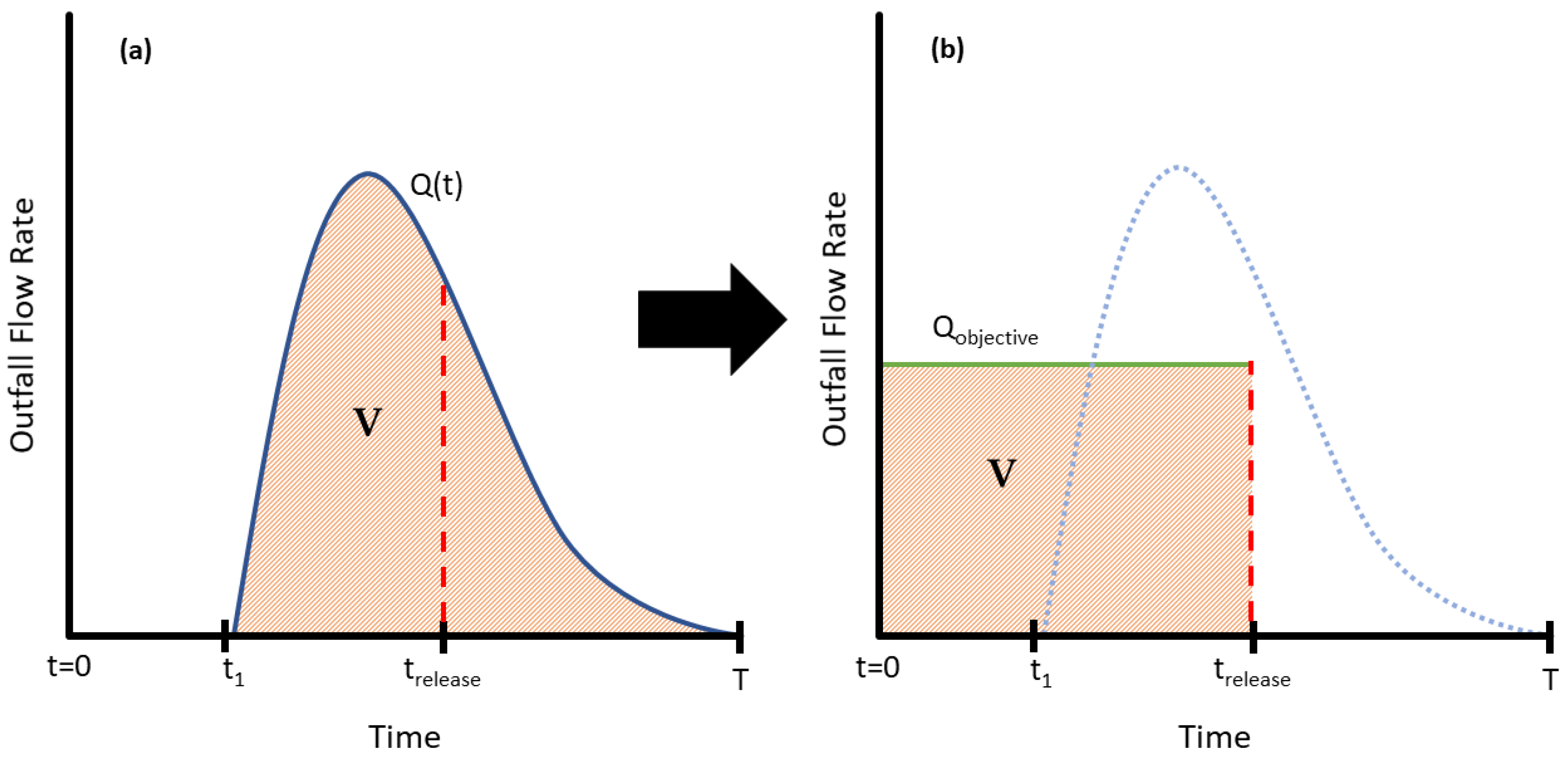
The essence of the optimization process is demonstrated in
Figure 1 with a simple rain event and its resulting hydrograph when no controlled releases were initiated (Q(t)). Given that the rainwater tanks were not empty at t = 0 and rain commenced at some point in time t
1, the following hydrograph Q(t) was recorded at the outfall of the drainage system (
Figure 1a). The total volume of overflows, or the total volume of wasted water V that cannot be used for supply can be calculated by
where T is the time when the flow at the outlet drops to 0.
The basic assumption of the presented optimization strategy is that for a given set of initial conditions and rainfall pattern, this volume V cannot be reduced when introducing controlled release. In other words, this volume V of water (or greater) will be conveyed through the drainage system in any controlled release policy. If V is assumed to be the smallest volume of rainwater to be conveyed through the drainage system for a given event, then in order to achieve the maximum reduction in peak flow of the simulated rain event, the flow at the outfall should be constant (denoted as Q
objective) and equal to
where t
release is the duration from t = 0 until controlled releases are stopped. This t
release was set to the time of the last recorded overflow of the simulation with no controlled releases (see “Simulation-Optimization Process”) used to find V (
Figure 1b). Because t
release is the last timestep with recorded overflow, it is selected as the timestep in which the controlled releases will stop as any release past the point in time of t
release is unnecessary (and any rain past this time will refill the tanks).
Naturally, Qobjective is synthetic and cannot be achieved from t = 0 to trelease (e.g., flow at the outfall cannot drop from Qobjective to 0 immediately), but the goal of the optimization process is to find a controlled release policy that will produce an outfall hydrograph as close as possible to Qobjective for every timestep of the simulation, since for every time period in which the flow at the outfall is smaller than Qobjective, there will be a resulting time period where the flow is greater than Qobjective.
Because the basic assumption is that V (the total volume of water conveyed through the system, which is the amount of wasted water) cannot be reduced, the optimization process also deals with the second objective of RWH—retain as much water as possible for supply.
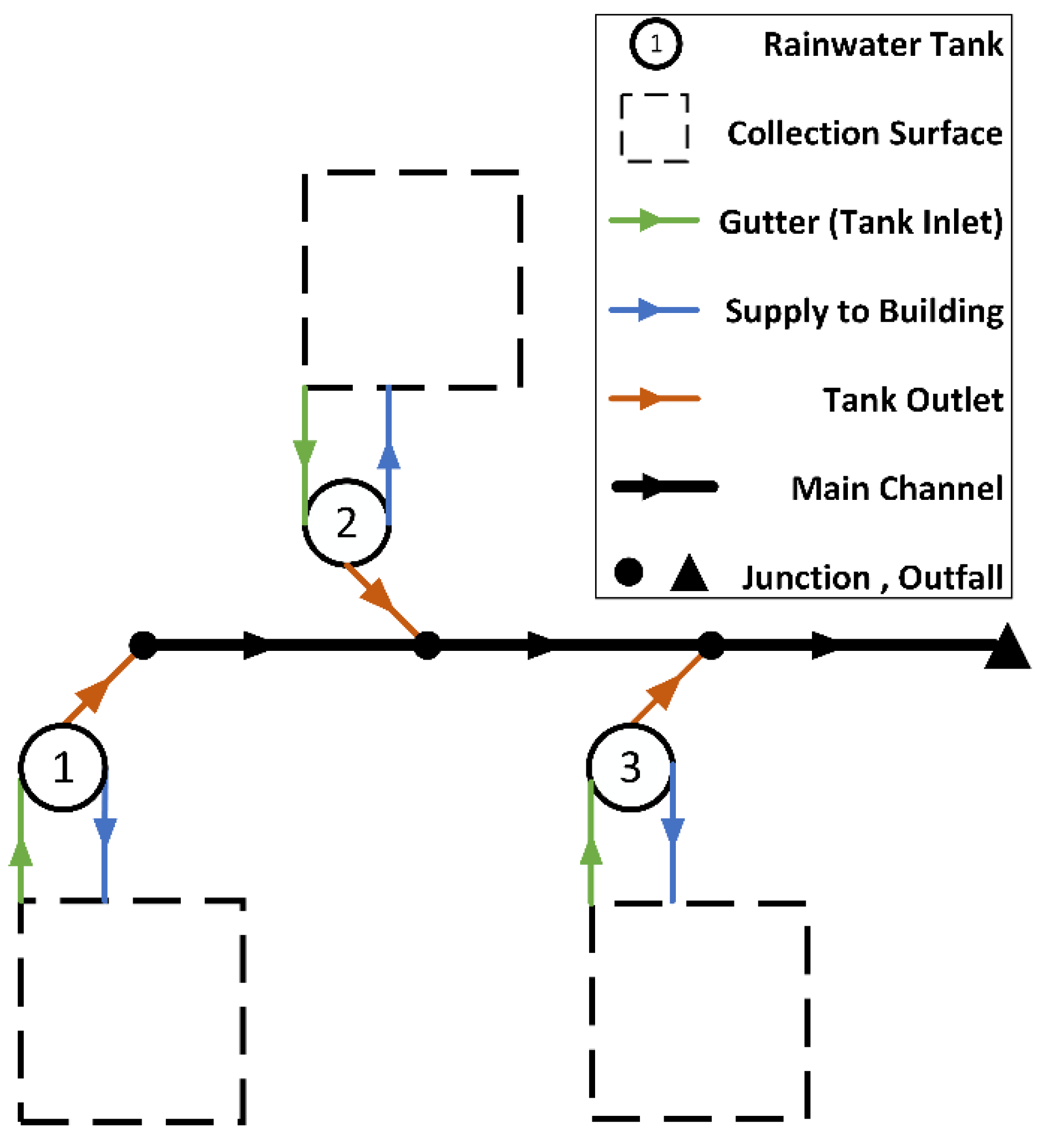
2.2. System Layout and Features
To test this optimization scheme, a simple dendritic drainage system was modeled (
Figure 2). The network consists of 3 RWH systems, each connected to a main channel through an outlet. The RWH systems and outlets are identical—to simulate RWH in high-rise residential buildings, each system collects runoff from a 1000 m
2 roof and serves a building with 150 tenants who have a deterministic water demand pattern. The modeled tanks have a capacity of 20 m
3, in correspondence with the findings of [
6,
28] regarding the reasonable tank volume for RWH in high-rise buildings in the Israeli climate.
There are 3 main channel conduits, the distance and slope between each junction of the main channel are equal, and the RWH system outlets and main channel conduits have a circular cross-section. The main features of the modeled system are presented in
Table 1.
2.2.1. Input Data and Storage Tank Mass Balance
For simulating the system’s response to a rain event, it is necessary to provide rainfall and demand data, which will be used to calculate inflows to and outflows from the rainwater tanks. To simulate overflows and changes in each tank’s storage, these inflows and outflows are used to solve a mass balance equation similarly to [
28]. This equation is solved according to the YAS (yield after spillage) principle [
29,
30]—inflows are calculated first, then overflows, controlled releases, and finally, yields from the tank.
For each timestep of the simulation, inflows to the tank are the rainfall depth for that timestep multiplied by the area of the collection surface. For simplicity, it was assumed that all rainfall is excess rainfall, which flows directly to the rainwater tank without depression losses. The rainfall data series that were used for this paper include logs from Beit Dagan meteorological station (32 N, 34.8 E), the oldest automatic rain station located in the Israeli coastal plain 10 km south-east of Tel Aviv. The rainfall data include two sets in 10 min resolution: (a) Intensity–Duration–Frequency (IDF) curves for 1-h and 2-h rain, and (b) three major rain events from the years 2000, 2010 and 2020. The IDF curves were simulated as constant rain for 1 and 2 h with the intensities presented in
Table 2:
Three real-life rain events were selected to test the efficiency of the proposed optimization scheme in response to different real rain patterns and intensities and are presented in
Table 3:
Demands from the tank are supplied in each timestep in which the tank holds sufficient water, so yields from the tank are equal to the smallest between the demands and the tank’s current storage. Demands in this work were set to include toilet flushing with a daily amount of 33 L per capita [
32,
33] with a diurnal pattern adapted from [
28,
34]. Demands were continuously drawn from the tanks (if water is available) during rainy and dry periods.
2.3. Flow Routing
The kinematic wave method [
35] was chosen to simulate flow routing from the tanks outlets down to the system outfall. Although the kinematic wave neglects the inertial components of the full dynamic wave equations [
36], it can be useful to simulate urban rainfall-runoff when the user acknowledges its limitations [
36,
37].
The kinematic wave model was applied by calculating the flow cross-section A at the inlet and outlet of each pipe (tanks outlets and main channel conduits) using Equation (3), an approximation to the flow–cross-section relationship [
38]:
where Q is the flow rate (m
3/s), A is the flow cross-section (m
2), and α, β are the kinematic wave parameters, equal to
where D is the pipe diameter (m), and S is the pipe slope (m/m) [
39].
These kinematic wave parameters were found to give a good approximation for the flow–cross-section relationship in circular conduits, better than the “classic” parameters proposed in earlier works [
38,
40] and adopted by [
41], and are applicable when the flow height is less than 90% of the pipe diameter [
39].
As flow at the tanks’ outlets is known (overflows and controlled releases are known for each timestep), the flow cross-section can be calculated at the entrance of each junction (
Figure 1). Inflows to each junction are the flow from the corresponding tank outlet and the flow that propagated down the main channel from the upstream junction.
To adjust the kinematic wave to the modeled system, the model was calibrated with the more accurate dynamic wave model used by SWMM using the PySWMM package [
42], where the calibrated variable is the simulation timestep (∆t).
2.4. Simulation—Optimization Process
The program was written in Python. Input data and scripts are available in Github. See
Supplementary Material.
The first stage of the optimization process is a benchmark run of the simulated rain event without controlled releases, so the network flows are generated from overflows only. This benchmark run is used to find V, trelease and Qobjective (Equations (1) and (2) above). The benchmark run also logs the peak flow at the outfall, the volume of supplied rainwater and the tank storage at the end of the simulation. For this paper, the benchmark run simulated the system’s response to the recorded rainfall.
2.4.1. Objective Function and Decision Variables
The objective of the optimization process is to produce a flow pattern as similar as possible to the constant value of Q
objective at the system outfall. To achieve this, the following objective function is used:
where i is the current timestep, n is the number of timesteps (determined by the simulation length and ∆t), Q
outfall(t) is the flowrate simulated at the system outfall. In practice, the absolute difference between the flow rate at the outfall and Q
objective is calculated at each timestep and is summed throughout the simulation run.
The decision variables for the optimization are the percentage of a valve opening at the bottom of each tank in 10% intervals (i.e., 0%, 10%, 20% etc.) as suggested by Di Matteo et al. [
17]. This approach ensures that the search space will only include feasible solutions. The valves can change their status at the beginning of each hour. As so, the number of decision variables is the number of hours until t
release rounded up and multiplied by the number of tanks. For example, if the last overflow from the tanks during the benchmark run was recorded in t = 9.5 h, then t
release = 9.5 h and the number of decision variables is 10 × 3 = 30. The flow rate from the tank valve is calculated by the orifice flow equation:
where Q
release is the flow rate from the tank due to controlled release (m
3/s), C
d is the orifice coefficient, A
orifice is the cross-section area of the orifice (m
2), g the gravitational acceleration (m/s
2), h is the water level in the tank (m) and Valve% is the valve opening percentage. It should be noted that Valve% refers to the orifice cross-section area and not the orifice diameter.
To calculate Qrelease, the following parameters were used for each tank: Cd—0.6; orifice diameter—5 cm; tank diameter—2.8 m (assuming circular tanks, the latter is used to determine h—the water level in the tank). Furthermore, the orifice is installed at the bottom of the tank.
2.4.2. Optimization Method
After the benchmark run is complete, a genetic algorithm package [
43] is initiated. Each “chromosome” is a complete policy of valve opening status for each tank for every hour of the simulated rain event. The fitness of each chromosome is evaluated according to Equation (5). To accelerate convergence, the initial population is seeded with a chromosome of all-zeros (i.e., all valves are closed throughout the simulation) and a chromosome that generates a policy of the valves constantly open at 10%. This, together with an elitism ratio of 2% [
44], ensures that the optimization process will find a release policy that is at least as fit as the benchmark run of no controlled releases. The optimal chromosome (i.e., the release policy that results in a flow pattern closest to Q
objective) was logged, together with the peak flow at the outfall, the total amount of rainwater used and the water storage in the tanks at the end of the simulation, so they could be compared with the corresponding logs from the benchmark run.
2.5. Result Evaluation
The optimal chromosome is evaluated by two parameters: (1) reduction in peak flow, and (2) reduction in rainwater availability (which equals the volume of rainwater used plus the storage in the tanks at the end of the simulations). Naturally, a favorable solution is one that reduces peak flows significantly while having minimal impact on rainwater availability.
To compare the performance of the proposed scheme with an established control method, the above-mentioned events were simulated with the predictive control method of releasing water from the tank when overflow is expected in a pre-determined forecast horizon [
13,
15].
This method was further developed by Snir and Friedler [
28], who suggested a new variable α to enable more flexible control over the release policy. α is defined between 0 to 1, and its value determines the fraction of water storage that will remain in the tank (e.g., α = 0.4 means that the release valve will be closed, and release will stop after the water volume in the tank decreases to 40% from its full capacity). This method enables the user to prioritize the system’s ability to supply water or to reduce peak flows—lower alphas mean more available storage prior to a predicted overflow, thus better ability to mitigate flows. Higher alphas mean keeping more water in the tanks, thus more water available for supply, but less free storage and higher overflows.
3. Results
To establish the optimization concept and test the resulting controlled release policies, the simulation-optimization process was first conducted with the IDF curve data as rain input with a 3-hour dry period before each simulation, where the tanks are full at t = 0. As the controlled release policies are in 1-h resolution, the resulting policies of the 1-h rain data were four decision variables for each tank—one for each hour of the dry period and another to the 1 h of rain. In the same way, the 2-h rain inputs resulted in deciding on 5 valve openings for each tank—three for the dry period and two for the rainy duration.
After the establishment of the process on the above-mentioned simple synthetic rainfall data, the real-life rain events described in
Table 3 (above) were used as input. To test the scalability of the optimization process, no changes were made to the program. The rain events were used as-is without a preliminary dry period, but the tanks were set to be empty at t = 0 (which is expected after 3–5 days of dry weather).
3.1. IDF Curve Rainfall
The optimization process was run for the rain intensities from
Table 2. The rain was modeled as constant rain for 1 and 2 h with a 3-h period of no rain at the beginning of each simulation, and all tanks were at their maximum capacity of 20 m
3 at t = 0. The effects of applying the release policy generated by the optimization process are presented in
Table 4. These effects include the reduction in the peak flow recorded at the outfall and the reduction in available rainwater due to the controlled release. The latter is calculated by adding the total amount of supplied rainwater to the overall water stored in the three tanks at the end of the simulation. The full results of the simulations, including recorded peak flows and rainwater availability, are available in the
Appendix A (
Table A1).
The reduction in rainwater availability was negligible in every simulation, with a maximum reduction of 1.4%. Moreover, controlled release policies for high and moderate probabilities were able to substantially reduce peak flows. However, implementing controlled releases does not improve the system’s ability to reduce flows in continuous and intense rain events such as the 1-h rain of 1% probability and the 2-h rain of 2% and 1% probabilities. The optimized release policies fail to overcome RWH’s known shortcoming of dealing with such rain events, especially considering that the synthetic rainfall inputs have no intermissions, which release policies might capitalize on to empty the tanks. This principle is apparent in
Figure 3 and
Figure 4, which present the optimized outfall flow patterns and the release policies that produced them. The figures present the results of a constant rain event with a probability of 5%—
Figure 3—an event of one hour with rain intensity of 39.9 mm/h (or 6.65 mm/10-min), and
Figure 4—an event of 2 h with rain intensity of 25.1 mm/h (or 4.18 mm/10-min).
The simplicity of the rain event and the fact that the release timesteps are 1 h in duration means that the solution can be divided into two time periods: before the rain begins and during the rainy hour. To maintain a flat flow pattern as much as possible, the solution empties the tanks gradually until the rain begins at t = 3 h—tank 2 empties first, then tank 1 and tank 3, the closest to the outfall, empties last. During the rainy hour, the valves are open at the mid-range values of 40–70% and are used to throttle the flow and are managing to do so until all the tanks are full at t = 3.8 h. The attenuation effect of the drainage network is preventing the flow at the outlet from reaching a steady flow of 33 LPS as in the benchmark run, even though the outflows from the tanks between t = 3.8–4 h are equal to those of the benchmark run. This means an 18% reduction in the peak flow.
The solution of the 2-h rain event displays a similar pattern of gradually emptying the tanks prior to rainfall. However, there is a possibility to change the valves’ opening settings at halfway of the rainy period—t = 4 h. This gives more flexibility to the solution, which the algorithm utilizes by opening the valves to the range of 70–100% during the first hour, and then closing them to 10–40% during the second hour. This causes a decrease in the flow during the first half of the 5th hour until the tanks are full, when as in the 1-h event, the attenuation effect of the system prevents the outfall flow rate from reaching a steady state until the rain ends, and the solution manages to decrease the peak flow by 15%.
3.2. Real Rain Events
To test the suggested control concept, the algorithm was run on three recorded rain events, which are described in
Section 2.2.1 and in
Table 3. The program was run without any modifications besides changing the rainfall input and setting the initial storage of each tank to 0 in order to simulate a rain event with a preceding dry period (very common in the Mediterranean climate). Results for peak flow reduction and the impact on available rainwater are presented in
Table 5. The full results of the simulations, including recorded peak flows and rainwater availability, are available in the
Appendix A (
Table A2).
The optimized controlled release policies were able to substantially reduce peak flows in all three events, with a significant impact on available rainwater only in the 2010 event.
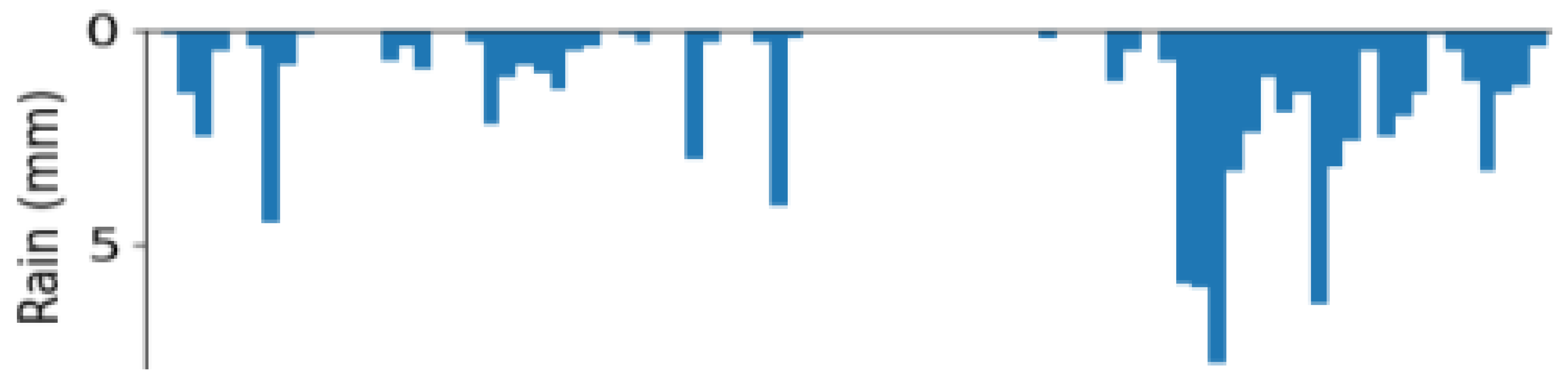
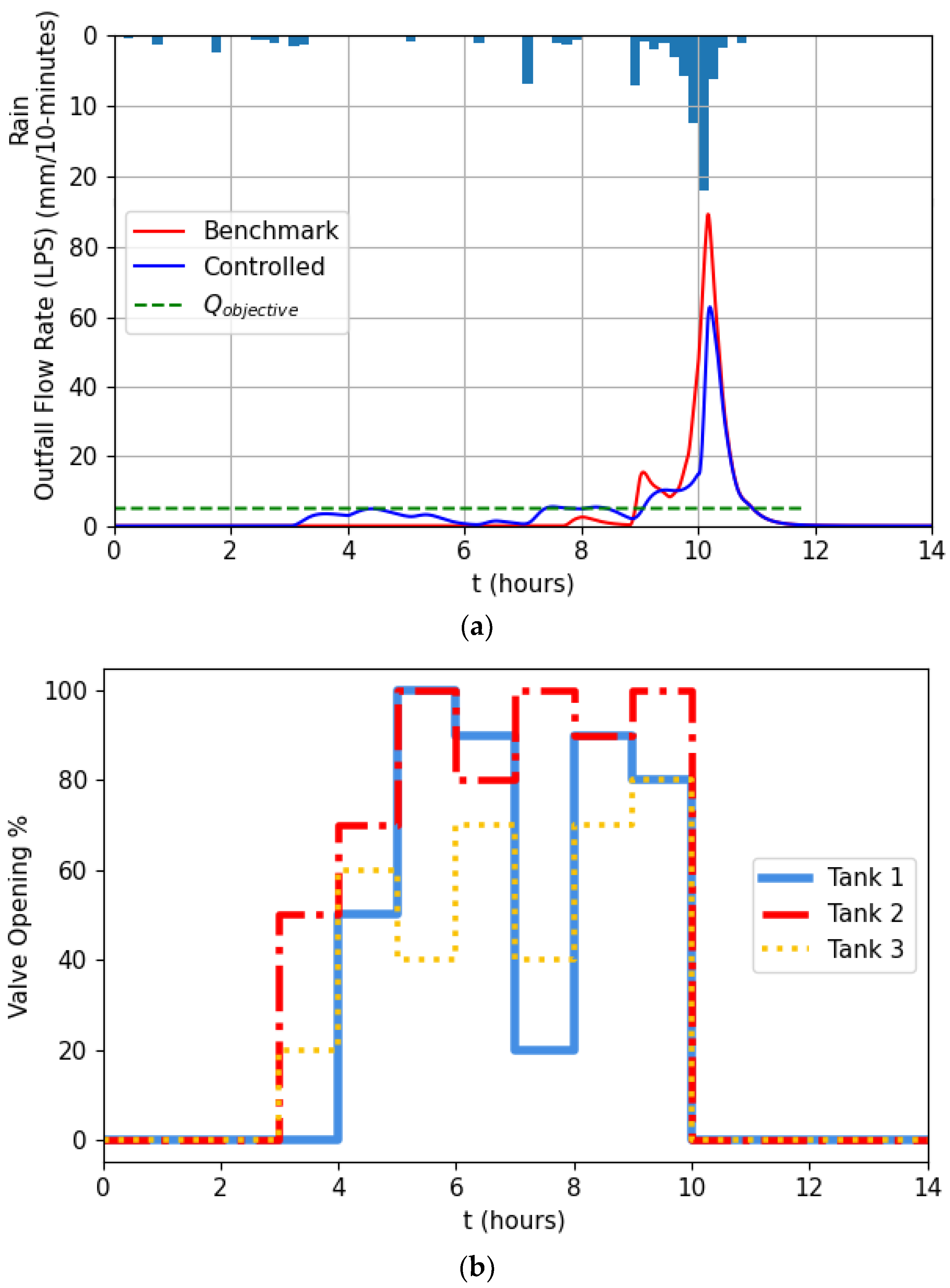
3.2.1. 5 January 2000
With a total of 87.9 mm recorded in 14 h, this rainfall pattern consists of intermittent rainfall for approx. 7 h, a dry period 3 h and an intense shower of 60 mm in 4 h. In the benchmark run, the first period of rain filled the tanks as could be deducted from the rise in flow around t = 6 h (
Figure 5a). Demands during the dry period were not able to extract enough water from the tanks, and the intense shower caused a noticeable rise in flow at the outfall of the simulated system.
The optimized release policy started to release water from t = 0 h while maintaining a flat pattern similar to Q
objective (
Figure 5a,b). As a result, the tanks were not filled, and their storage did not surpass 40% of their full capacity (
Figure 5c). All three tanks were emptied until t = 8 h. During the first 2 h of the intense rainfall (t = 9–11 h), the valves’ opening percentages ranged from 70% to 100%, but were reduced at t = 11 h as the tanks had sufficient empty storage to handle the remaining inflows. This policy flattens the local maximum shortly before t = 12 h.
In total, the controlled release policy was able to reduce the peak flow at the outfall from 33 to 18 LPS while reducing the volume of available water from 67.4 to 65.2 m3.
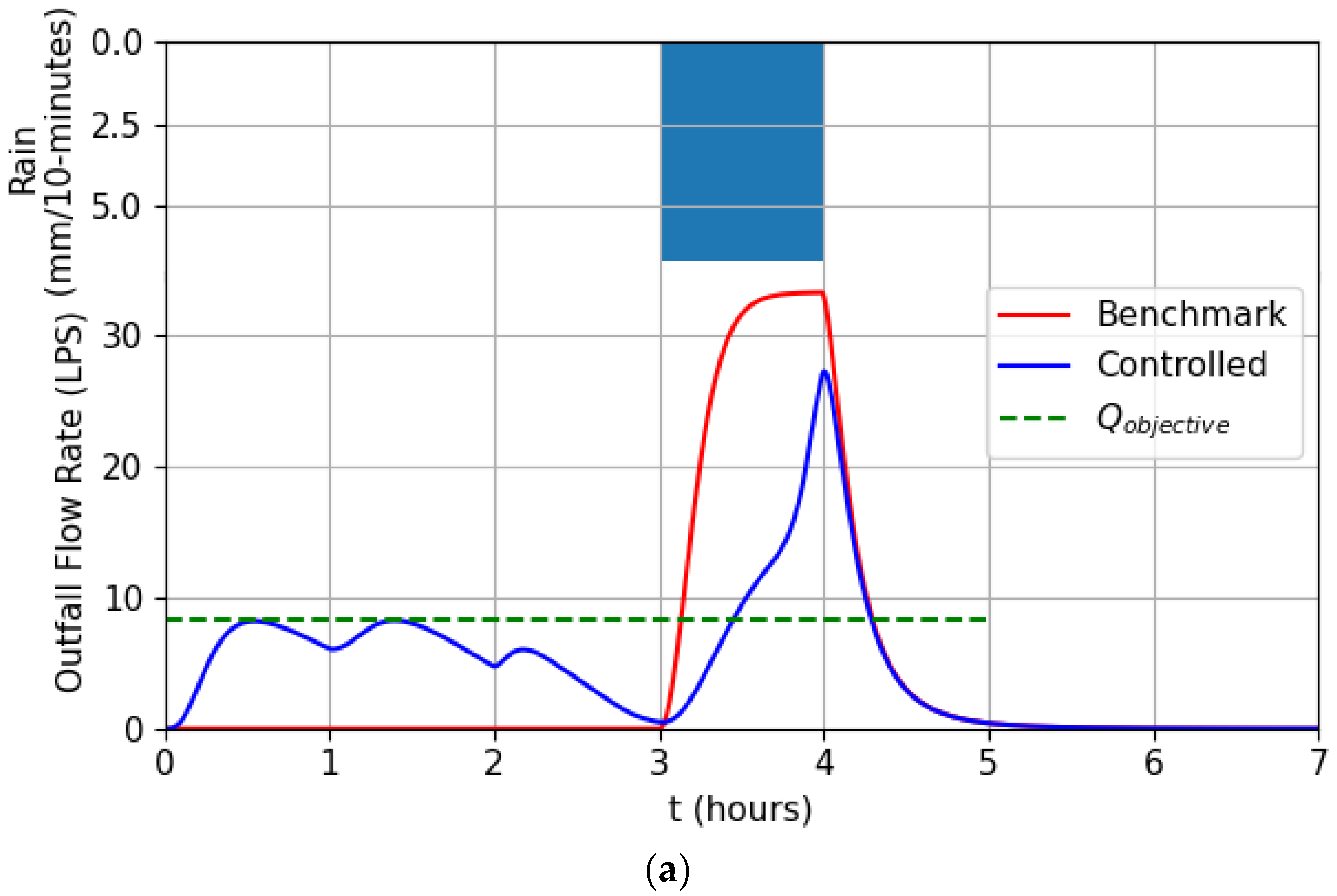
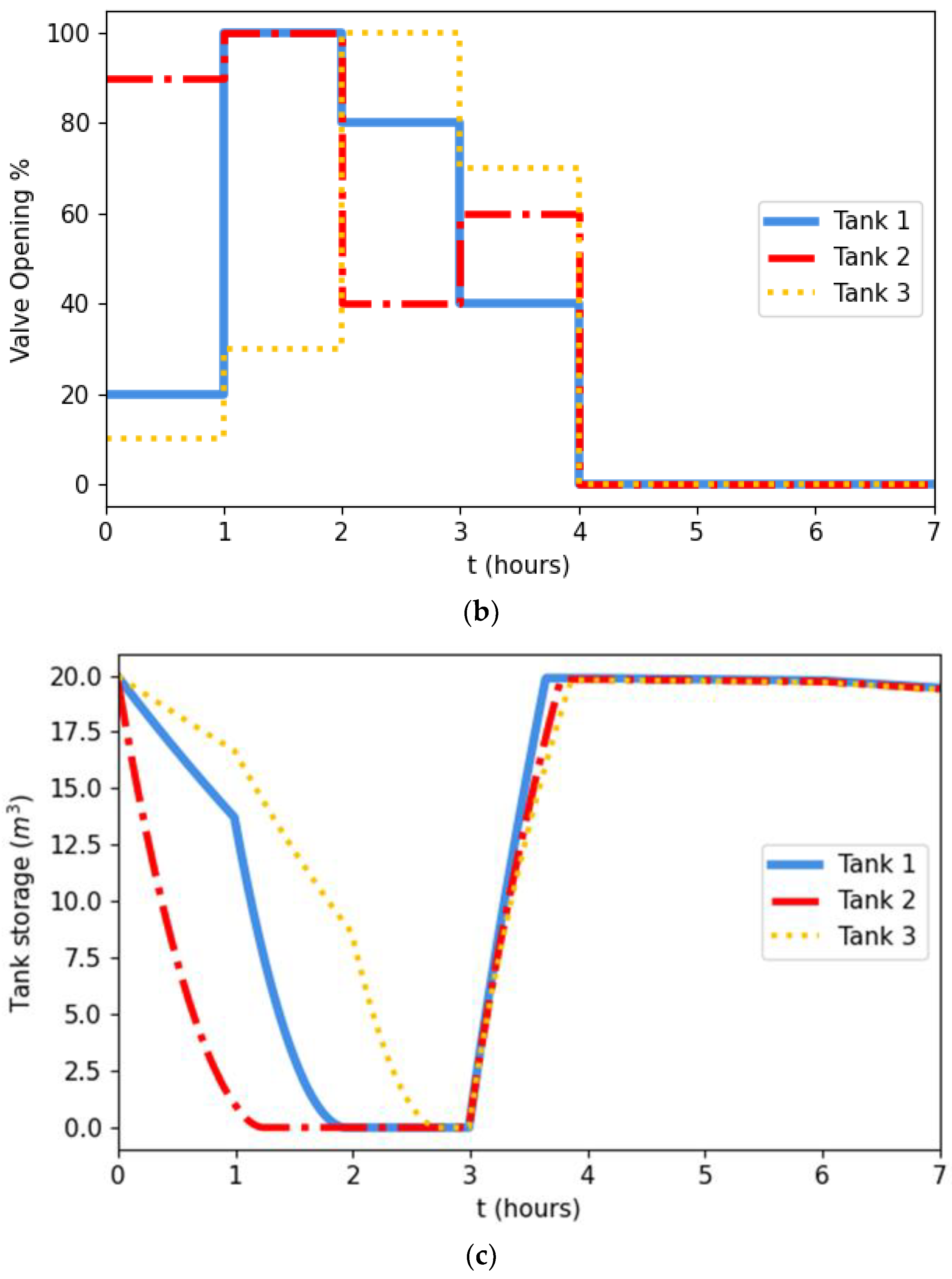
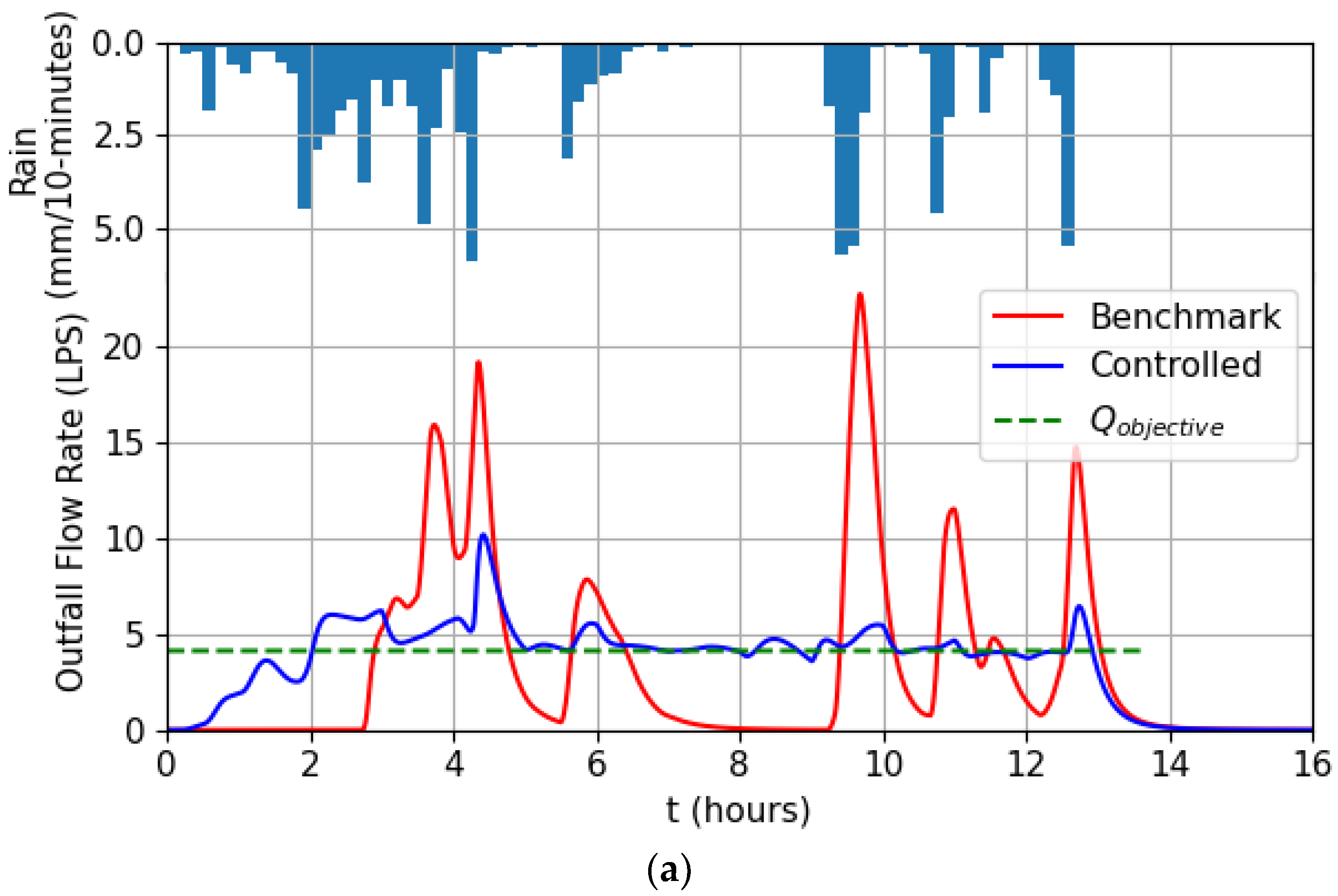
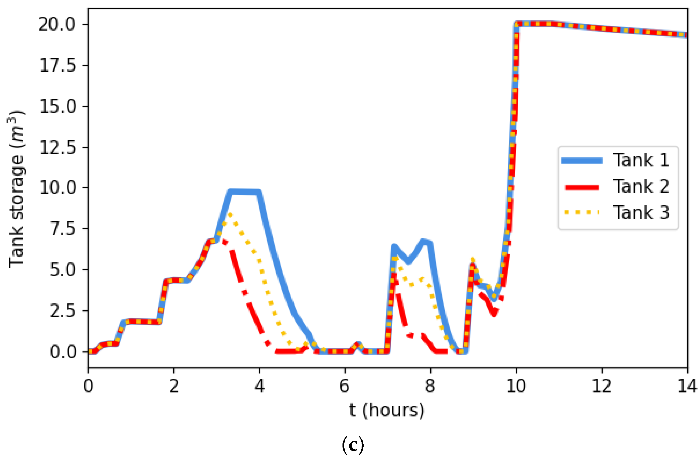
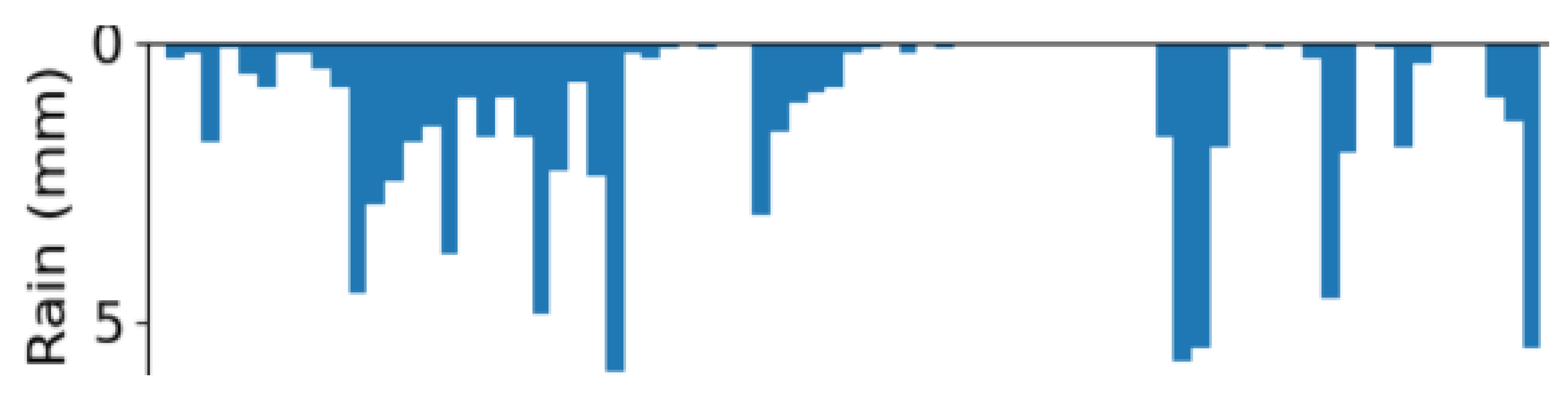
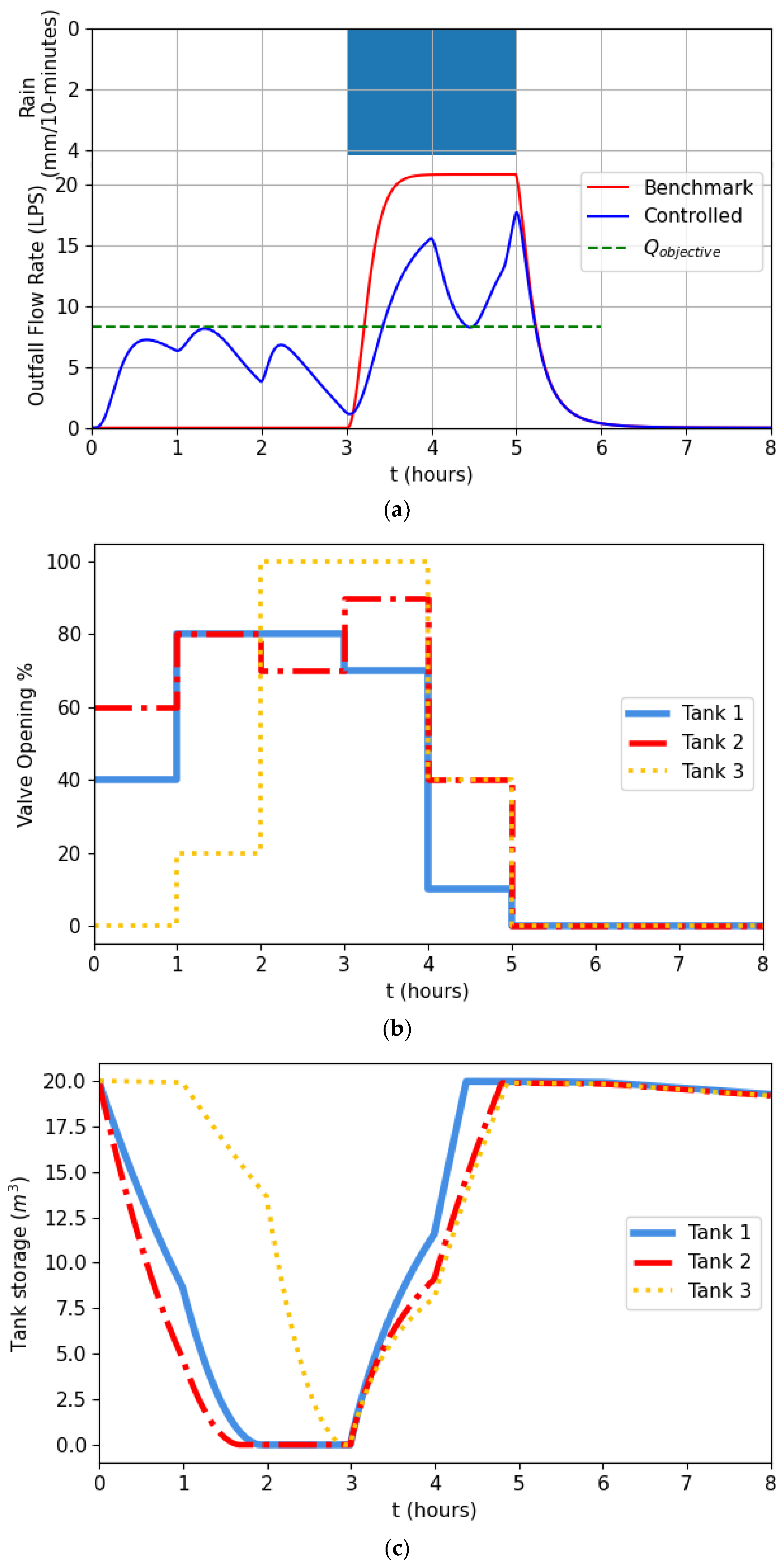
3.2.2. 25–26 February 2010
The 2010 rain event showed similar total rain depth and duration (85.1 mm and 13 h, respectively) to the 2000 event, but with a significant shower starting in t = 0 h until t = 6.5 h. After an intermission of 2 h, 4 bursts of rainfall were recorded with short breaks between them (
Figure 6a). With no controlled release, the tanks were filled by t = 3 h and remained full throughout the event, and the peak flow at the system’s outfall was generated during the first rain burst after the intermission before t = 10 h (
Figure 6a).
The controlled release policy opted towards significant releases in the first 2 h of the event, presumably to avoid the high flows right before and after t = 4 h, which occurred in the benchmark run (
Figure 6b). This course of action led to the tanks being full only after t = 4 h (
Figure 6c), in comparison to t = 2 h during the benchmark run, and to a significant reduction in flow during the initial rain shower. The controlled release policy almost completely emptied tanks 1 and 2 during the intermission but kept the valve of tank 2 at an opening percentage of 10% from t = 9 h onwards, which caused it to be the only full tank at the end of the rain event at t = 13 h. The fact that tanks 1 and 3 were not full by the end of the event caused a significant impact on the rainwater availability, reducing it by 25% in comparison to the benchmark run.
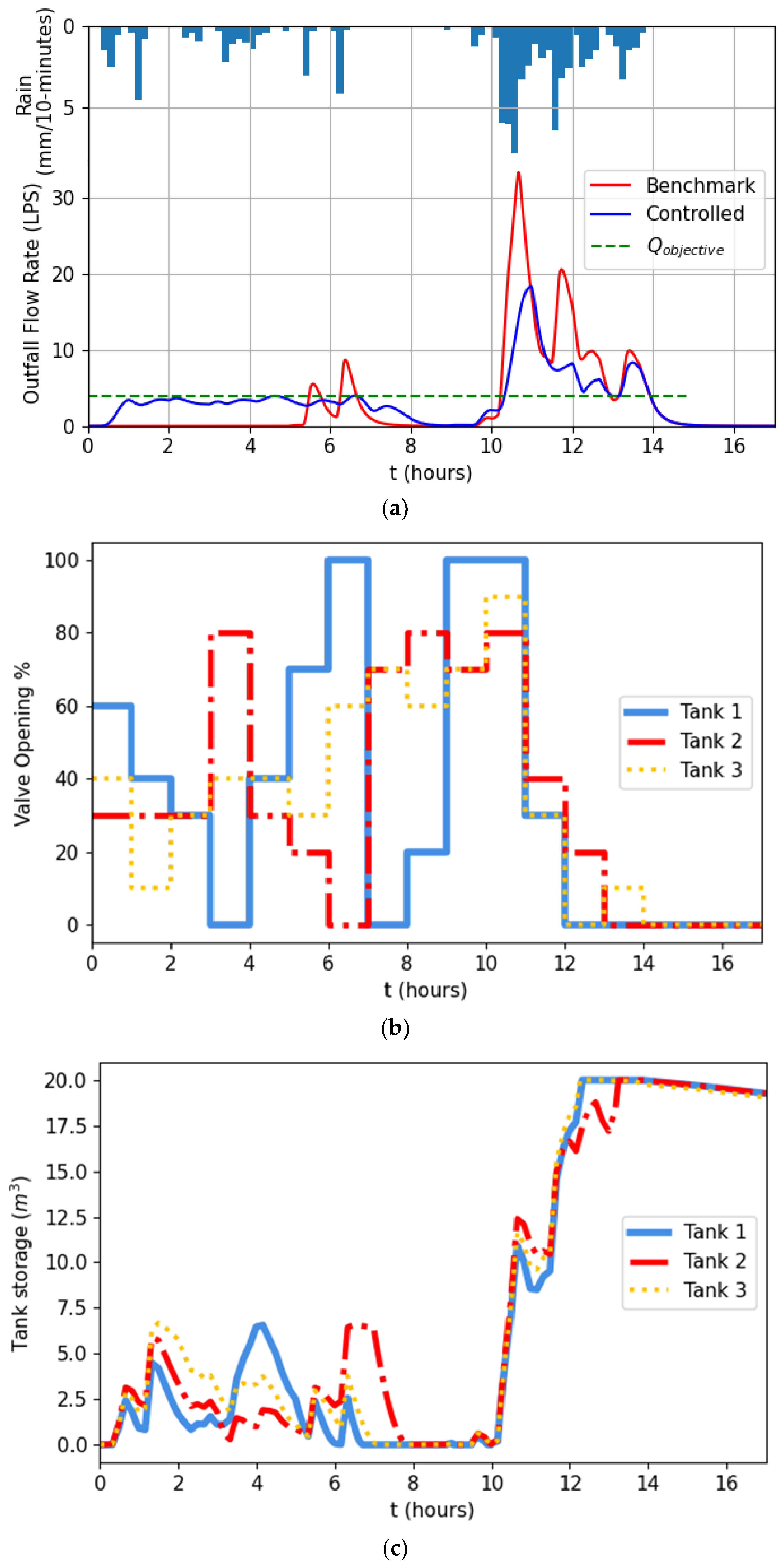
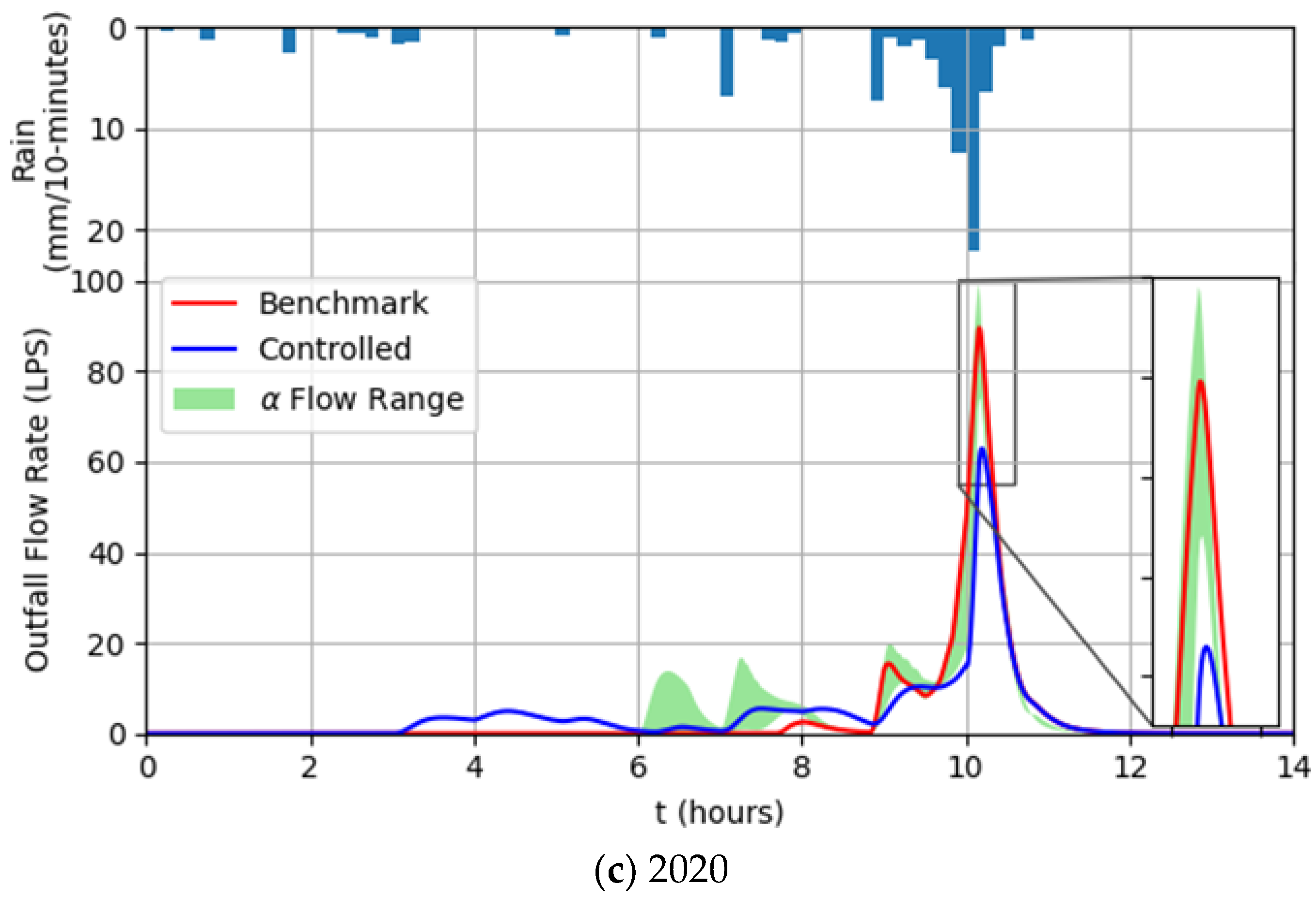
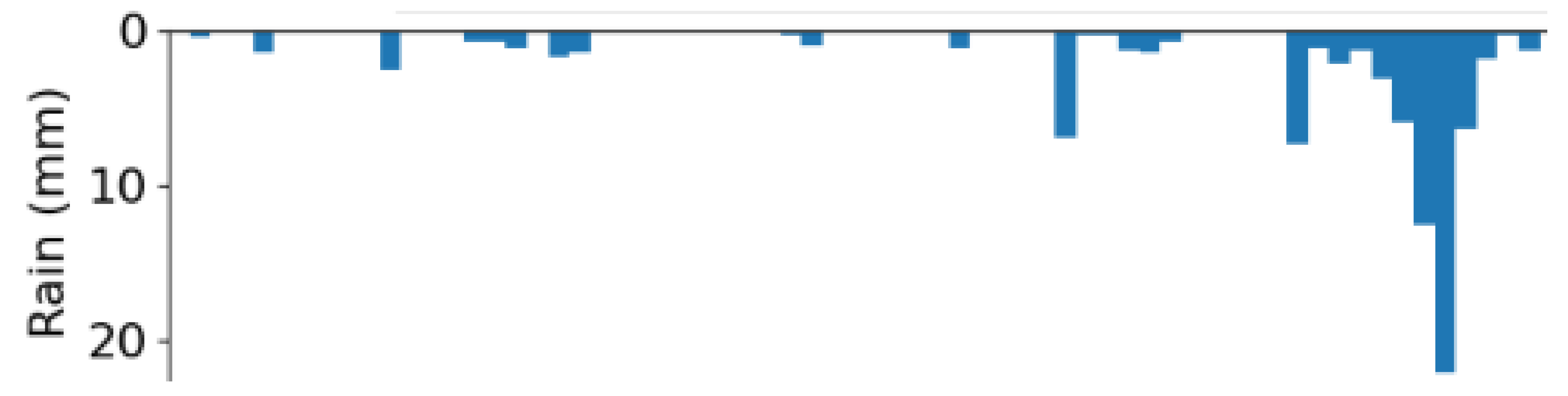
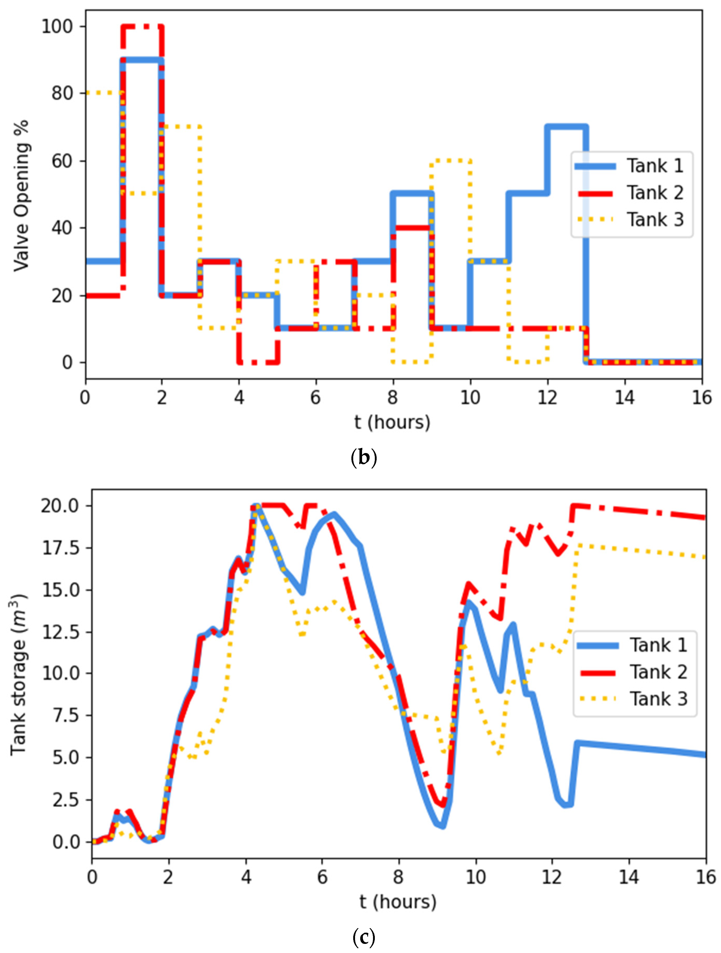
3.2.3. 20–21 November 2020
The rain system of November 2020 was one of the most intense in Israeli rainfall records, although spatially limited mostly to the mid-northern coastal plain. With some areas receiving more than 200 mm in less than 48 h, the system caused both pluvial and flash floods across the coastal plain [
31]. Although the total measured rain depth in Beit Dagan meteorological station was only 104.7 mm, 51.7 mm was recorded in just one hour, of which 41 mm was recorded in just 30 min. The simulated rain event included this period of intense rainfall.
The simulated event has similar total depth and duration to the previous events (87.4 mm and 11 h, respectively), but as mentioned, displays a short period of extreme intensity after 9 h of sporadic showers (
Figure 7a). These early showers were able to fill the tanks and cause overflows by t = 8 h as indicated by the rise in the outfall flow recorded during the benchmark run (
Figure 7a).
The release policy main objective in this event was to keep maximum available storage free before the intense shower starts at t = 9 h. This was achieved as can be seen in
Figure 7c—the tanks were full only after 10 h in comparison to 8 h in the benchmark run. This enabled better control of the incoming flows and a reduction of 30% in the peak flow recorded at the outfall.
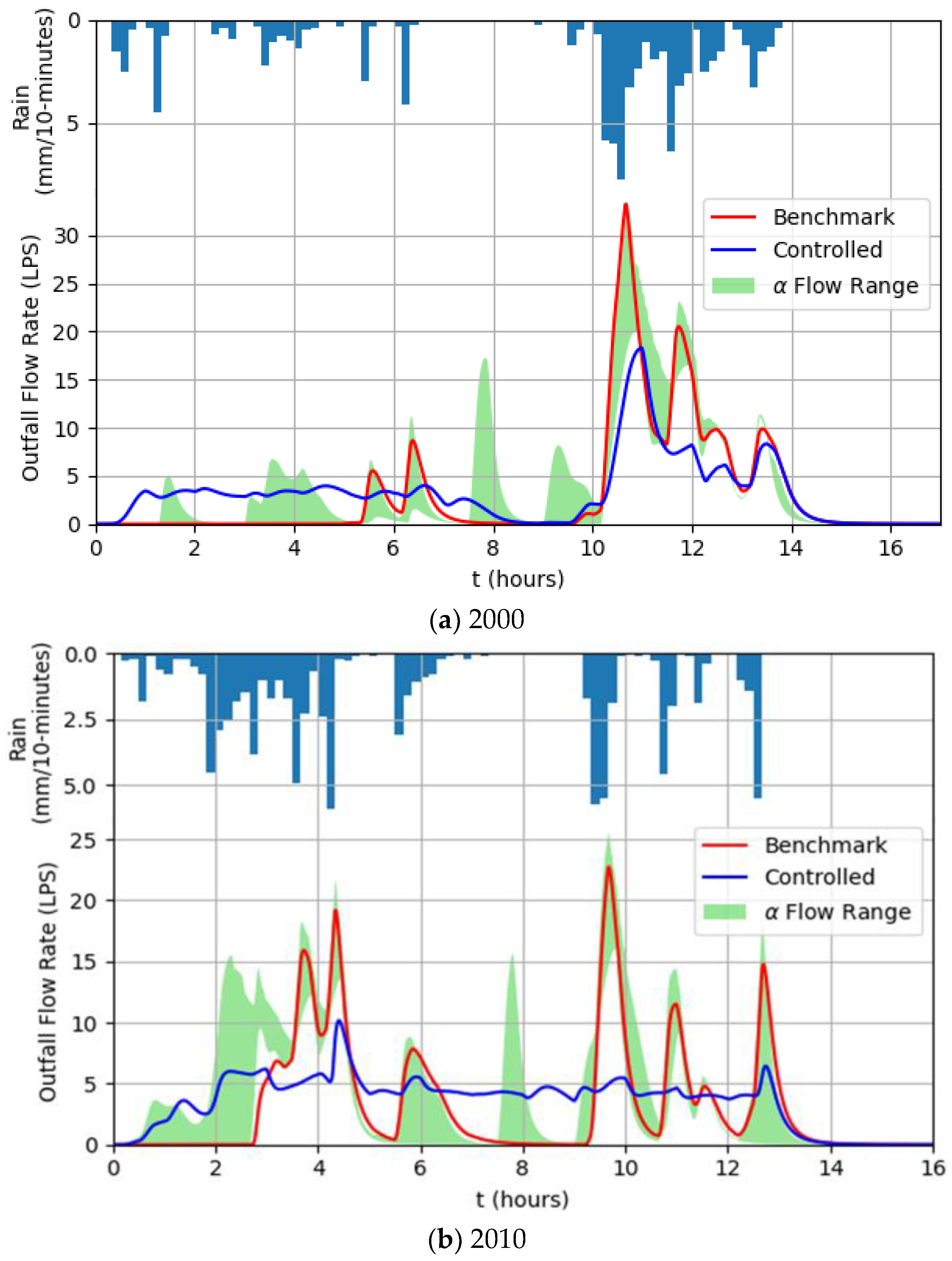
3.3. Comparison with the Alpha Releases Method
To compare the α method to the current scheme, 10 different alphas between 0 to 0.9 were examined in each of the three measured rain events. To reduce the number of presented results and to exclude any possible bias that might occur when choosing specific alphas, peak flow reduction and rainwater availability reduction resulted from the proposed optimization process will be compared with the highest peak flow reduction and the lowest rainwater availability reduction that resulted in running the full range of alphas. Naturally, the best peak flow reduction was achieved when setting α = 0 (leaving no water in the tanks) and the lowest rainwater availability reduction was achieved when setting α = 0.9 (leaving 90% of each tank’s water storage).
As presented in
Table 6, the proposed optimization method outperformed the α parameter method even with choosing the best results from the entire range of the latter, except from the high impact on rainwater availability the former had in the 2010 event. This advantage is further demonstrated in
Figure 8, where the flow patterns resulting from the benchmark runs and the optimized control policies are plotted with the full range of flow patterns created by the α parameter method. This range was plotted by finding the maximum and minimum flow of the entire α range (0–0.9) in each timestep, i.e., the top and bottom bounds of the shaded area are not a result of a single value of α.
As shown by Snir and Friedler [
28], the α parameter method can reduce peak flows significantly, but with a price of reducing rainwater availability, especially with lower alphas. However, the suggested optimization method manages to reduce peak flows more efficiently, especially when the rain event is characterized by multiple local maxima in flows such as the 2010 storm. Moreover, unlike the suggested policy optimization method, which opts to flatten the flow pattern, using the α method might introduce surges in flows caused by the releases themselves, as seen in
Figure 8a at t = 9 h and in
Figure 8b at t = 2 h and t = 8 h. It should be noted again the shaded area and its bounds do not represent a single value of α. An example of this can be seen in
Figure 8b between t = 7–10 h—it is not possible to produce a flow pattern that is characterized with the lower bound of the α flow range shortly before t = 8 h and the lower bound shortly before t = 10 h. The first is a result of a higher α—less water is released prior to the expected overflow, but the latter is a result of lower α, which released more water before the storm.
4. Discussion
4.1. Objective Function
RWH and RTC of RWH systems are set to achieve two objectives: (a) Save potable water and (b) mitigate peak flows in the urban drainage system; the latter can also include basin baseflow restoration in its broader sense [
15,
16]. As these two objectives often compete, active decisions about whether to release or hold rainwater should be a result of multi-objective optimization in order to fully comprehend the actual costs and benefits of such decisions. However, multi-objective optimization usually requires putting the objectives on level grounds by examining weights on each objective or to reveal a range of optimal solutions without making actual decisions by finding a Pareto front [
45]. Thus far, research on the dual benefit of RWH was limited to optimizing only one objective (e.g., minimizing peak flows [
17,
18]), demonstrating the cost in potable water savings when applying RTC to mitigate peak flows [
13,
15,
16] or exploring ways to show a range of RTC solutions from which a stakeholder might be able to choose from (e.g., α parameter as a decision variable [
28]).
The main advantage of the proposed optimization method, and especially the objective function in its base (Equation (5)), is that it captures both objectives in one mathematical term, thus dismissing the need to assign weights to the different objective or generate Pareto fronts. By finding a control policy that generates a flow pattern as close as possible to Qobjective, the control policy aims to release a volume of water that is not greater than the volume of overflows without control release, as well as creating a flat flow pattern. Moreover, this method is scalable and could be easily adjusted to any rain event as demonstrated in this paper.
4.2. Constant Rain Intensities
To examine the policy optimization process, 10 different rain intensities from the Beit Dagan 1-h and 2-h IDF curves were used as input. As the rational method for calculating peak flows is still a common practice in Israel (although not very accurate [
46]), data from IDF curves is the common input for designing and examining various aspects of urban drainage systems. This, together with the relative simplicity of the rainfall patterns, were the reasons to firstly examine the suggested optimization method on this type of input.
Intuitively, the method of mitigating flows generated from a steady rainfall shower is to empty the storage units right before the rain starts (assuming that the storage units are not empty at the beginning of the simulation). The suggested algorithm was opting for this strategy in all of the simulations. The algorithm also tended to keep the valves open during the storm, and by that, releasing water from the tanks with a flow lower than the overflow, which would have occurred if the tanks were full. This way of throttling the flow kept the tanks from filling up quickly, thus managing to further reduce the simulated peak flow.
However, constant rainfall, which is rare in reality, gives no intermissions for the algorithm to take advantage of, and insignificant peak flow reductions were achieved in trying to cope with higher (and rarer) rain intensities.
4.3. Recorded Rain Events
In contrast to the constant rain intensity simulations, the input of actual rain events allowed the algorithm more flexibility in managing storage and flows. An example could be seen in the rain event of 2010 (
Figure 6)—during the last 2 h of the first rain shower (t = 2–5 h), the release policy opted towards a small opening percentage of the valves, thus allowing the tanks to fill and overflow. However, this enabled the constant release of water throughout the 3 h intermission without completely emptying the tanks and better handling the second part of the rain event from t = 9 h onwards. This behavior shifted the recorded peak flow from t = 9.5 h during the benchmark run to t = 4.5 h and allowed a significant improvement in peak flow reduction in comparison to the α parameter method (
Figure 8b).
The advantage of the suggested policy optimization method over simply releasing water prior to an expected overflow is apparent in all simulated events. The writers believe that the reason for this advantage is the manner of finding Qobjective, the key variable in the objective function. Qobjective is calculated using the system’s response to a specific rain event. By considering the outfall flow rate function and the total time of the event (Equations (1) and (2)), Qobjective is tailored to find the optimal flow pattern of a specific system to a specific rain event and includes all influencing parameters such as collection surface area, demands from the rainwater tanks, tanks’ capacity, drainage system layout and design, and the rain event’s pattern and intensity.
4.4. General Discussion and Future Research
As aforementioned, the presented approach tends to make use of intermissions between showers and achieves lesser results when dealing with constant and steady rainfall. This behavior is an advantage when applied to Israel’s typical rainfall patterns, which tend to be a result of cold fronts and thus scattered with high temporal and spatial variability.
However, this variability increases the algorithm dependency on accurate rain forecasts. As explained in the “Methods” section, the presented method is regulating the rainwater tanks according to a benchmark run. The results presented here are the outcome of a process that uses the same rainfall data for optimization and for the solution evaluation, thus simulating rain events with perfect knowledge of the rainfall’s depth and temporal distribution. Future work should simulate more realistic scenarios where the benchmark run and optimization are executed with rain forecasts that do not fully correspond with the measured rainfall data. This will introduce uncertainty and risk, which will probably reduce the algorithm efficiency. However, this reduction could be mitigated by various methods within the field of RTC of drainage systems [
47], including the implementation of Model Predictive Control (MPC) [
24,
48,
49] where the simulation-optimization routine is performed with a receding forecast horizon throughout the duration of the rain event, thus allowing to update the rain forecast as the event progresses.
As the scope of the presented work includes only rooftops as surfaces that contribute to runoff and drainage flows, another step towards more realistic simulations will be the modeling of an actual urban catchment, including pervious and non-previous areas that affect drainage flows, but their runoff is not collected by RWH systems. As the flows generated from these non-collectable areas cannot be controlled by regulating the valves of the RWH tanks, the writers believe that this step will not require significant alterations of the algorithm or the optimization scripts. Moreover, during examination of the generated control policies, the algorithm occasionally yielded different control policies, which resulted in similar flow patterns at the system outfall. It is assumed that due to the similarity of the modeled RWH systems (i.e., identical tank size and collection area), the optimized control policy is not unique in its fitness. It is expected that modeling more realistic catchments with variability between different RWH systems, in addition to more complex drainage networks with varying pipe diameters, slopes and lengths will result in significant differences between examined release policies.
Another possible development will be a temporal expansion of the optimization routine to simulate entire rainy seasons and to conduct pluriannual evaluations of peak flow reduction and rainwater availability, as conducted in [
28] for a single building.
5. Conclusions
This paper presents a proof of concept to a method of producing control policies for the centralized operation of a distributed network of RWH systems as a part of an urban drainage system. The suggested method utilizes the drainage system’s response to a given rain event, analyzes the flow pattern at the network’s outfall and aims to produce a new, flat flow pattern by regulating valves of the modeled RWH systems. This simulation-optimization procedure enables the use of a simple objective function, which accounts for both benefits of RWH—mitigation of peak drainage flows and alternative sources for domestic water consumption. As these two gains often compete, an optimization process that captures both without using weights or creating Pareto fronts might prove to be a useful tool in future research in the field of RTC of RWH systems.
After applying the suggested approach on a simple network of RWH systems and drainage conduits, the following conclusions could be drawn:
The process successfully utilizes dry intermissions between rain showers in order to flatten the flow pattern throughout the rain event.
When compared to a conventional RWH systems, applying the control policies generated by the suggested method significantly improves the system’s ability to mitigate high drainage flows.
When compared to other methods of controlled release, the suggested method outperforms in both peak flow reduction and rainwater availability.
To conduct more realistic simulations and assessments of the presented approach, future research will include:
Introducing uncertainty by using rain forecasts as input for the benchmark and optimization runs rather than the actual rainfall data and then comparing them ex-ante with real rainfall.
Modeling realistic urban catchments and drainage networks, in which different RWH systems have different attributes and drainage conduits vary in diameter, slope and length.
Introducing stochastic demand patterns rather than deterministic as suggested by Snir and Friedler [
28].
Although applying these developments is likely to produce less favorable results than those portrayed in this paper, their implementation will bring about further improvements to the algorithm and the development of the field of centralized control of decentralized RWH systems in general.


