
Concurrent Changes in Extreme Hydroclimate Events in the Colorado River Basin


Abstract
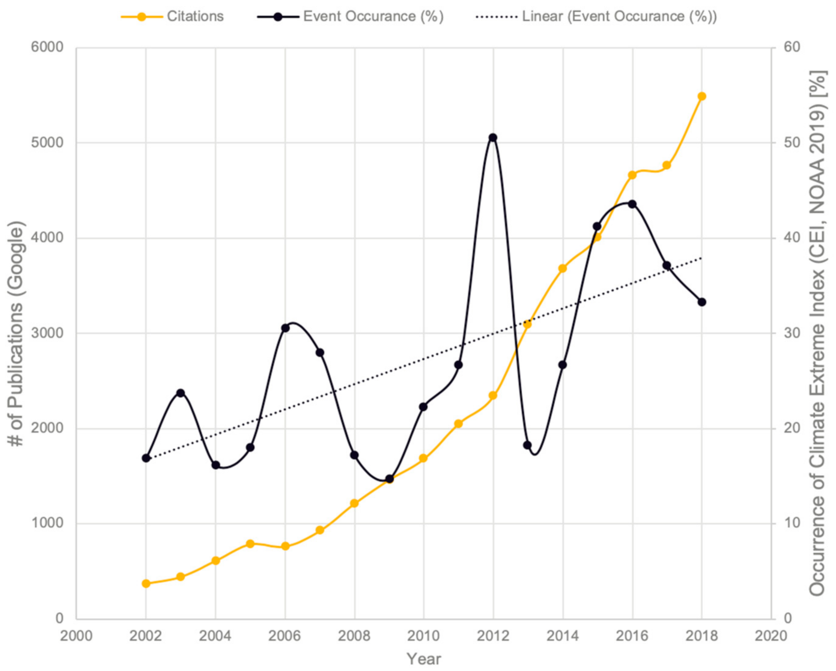
1. Introduction
2. Materials and Methods
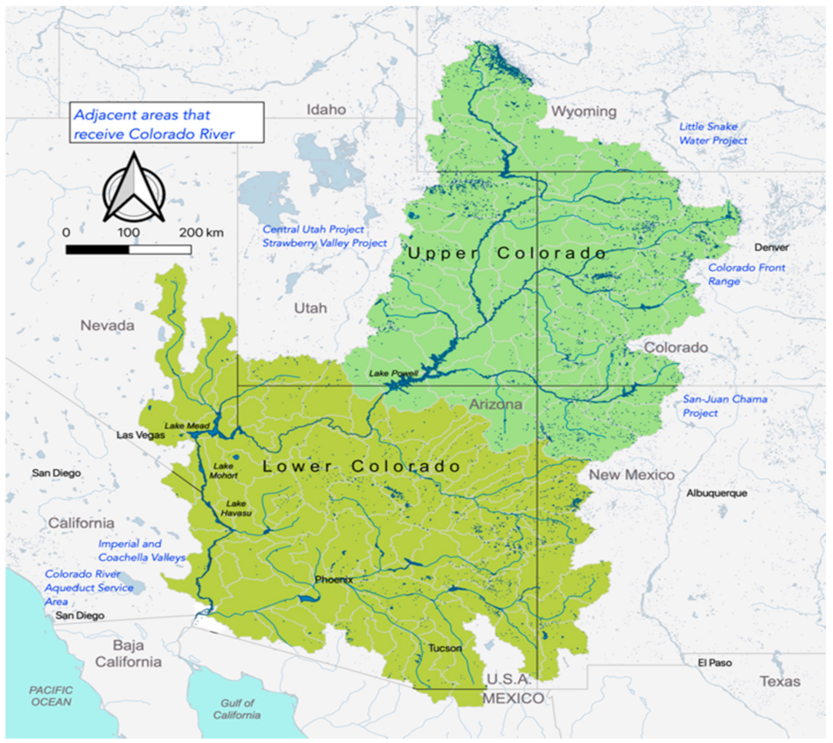
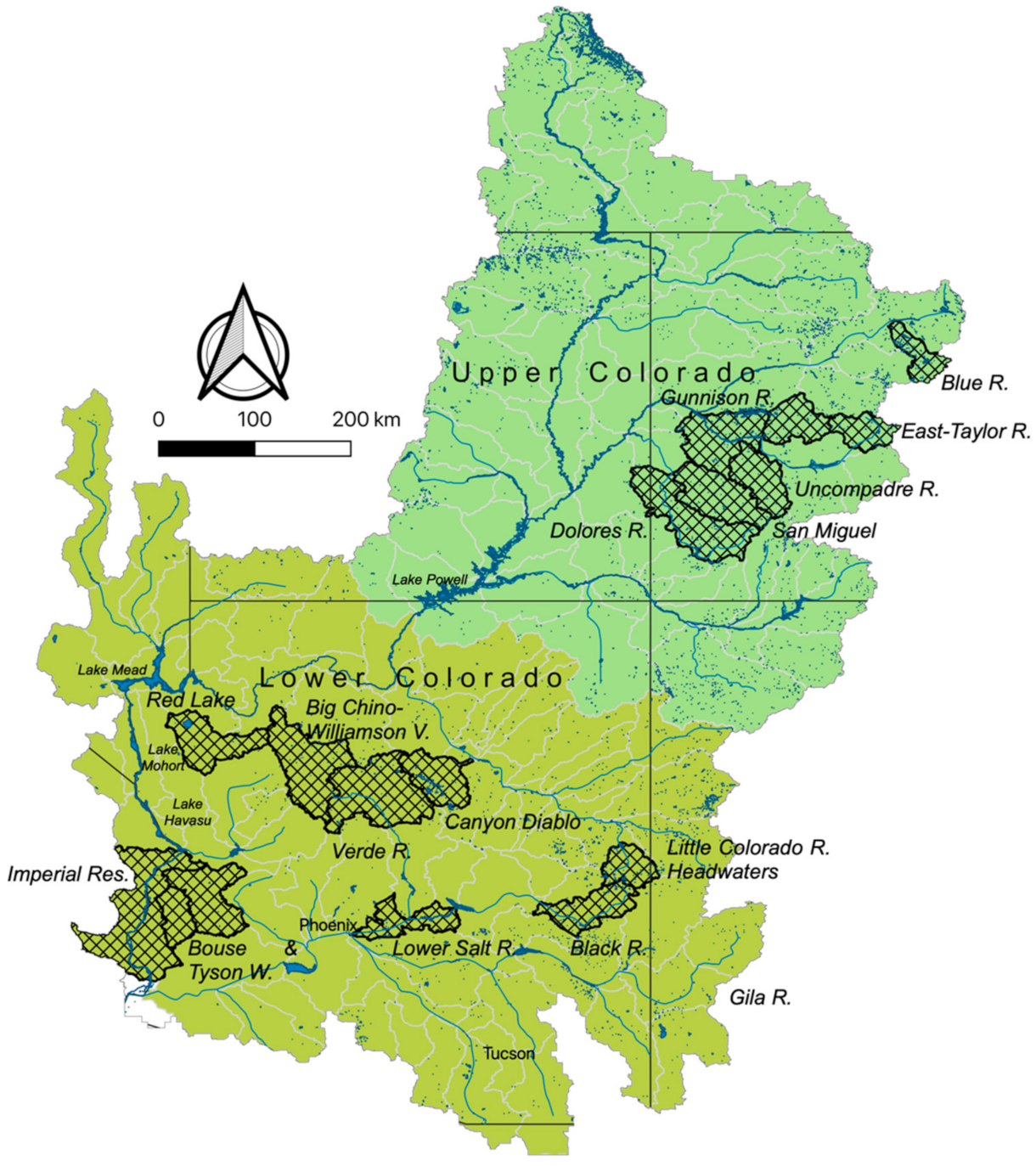
2.1. Study Site
2.2. Climate Simulations
2.3. Hydrological Simulations
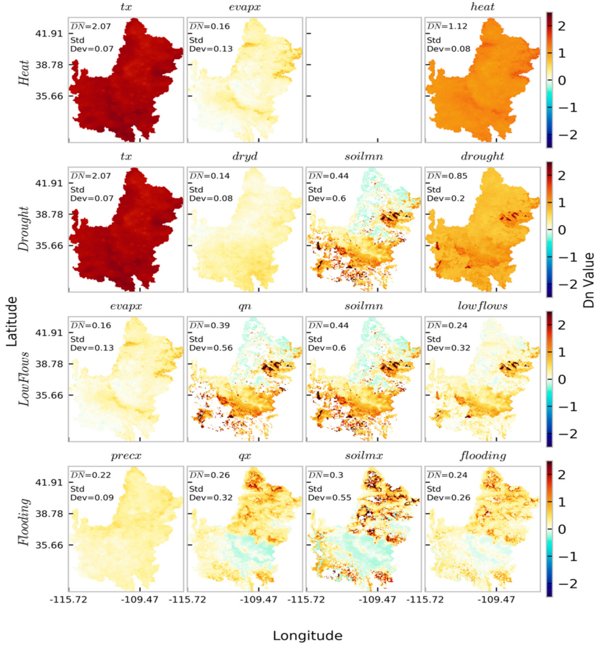
2.4. Extreme Indicators and Impacts
2.4.1. Peaks Over Threshold Extreme Exceedance
2.4.2. Distance Number
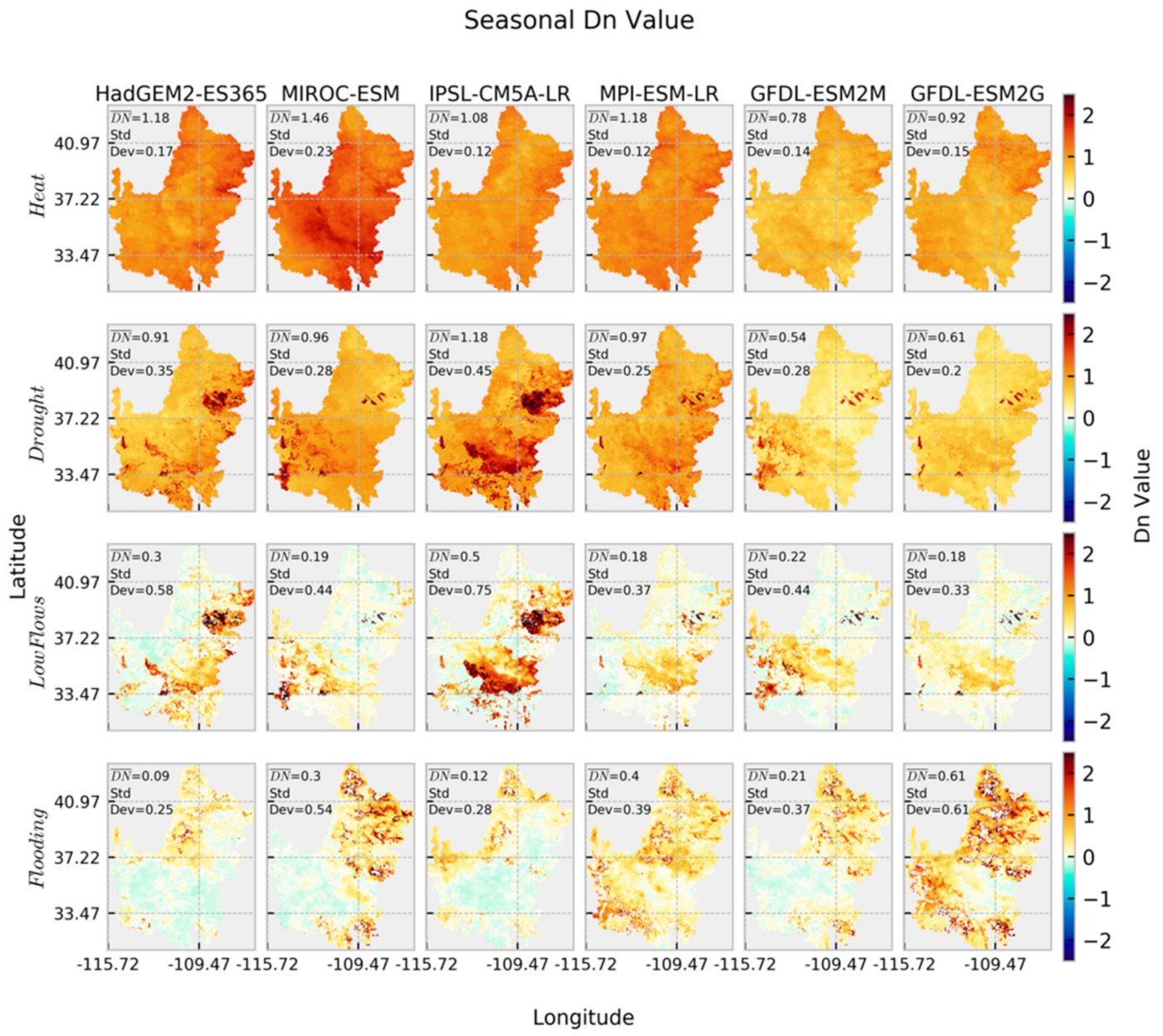
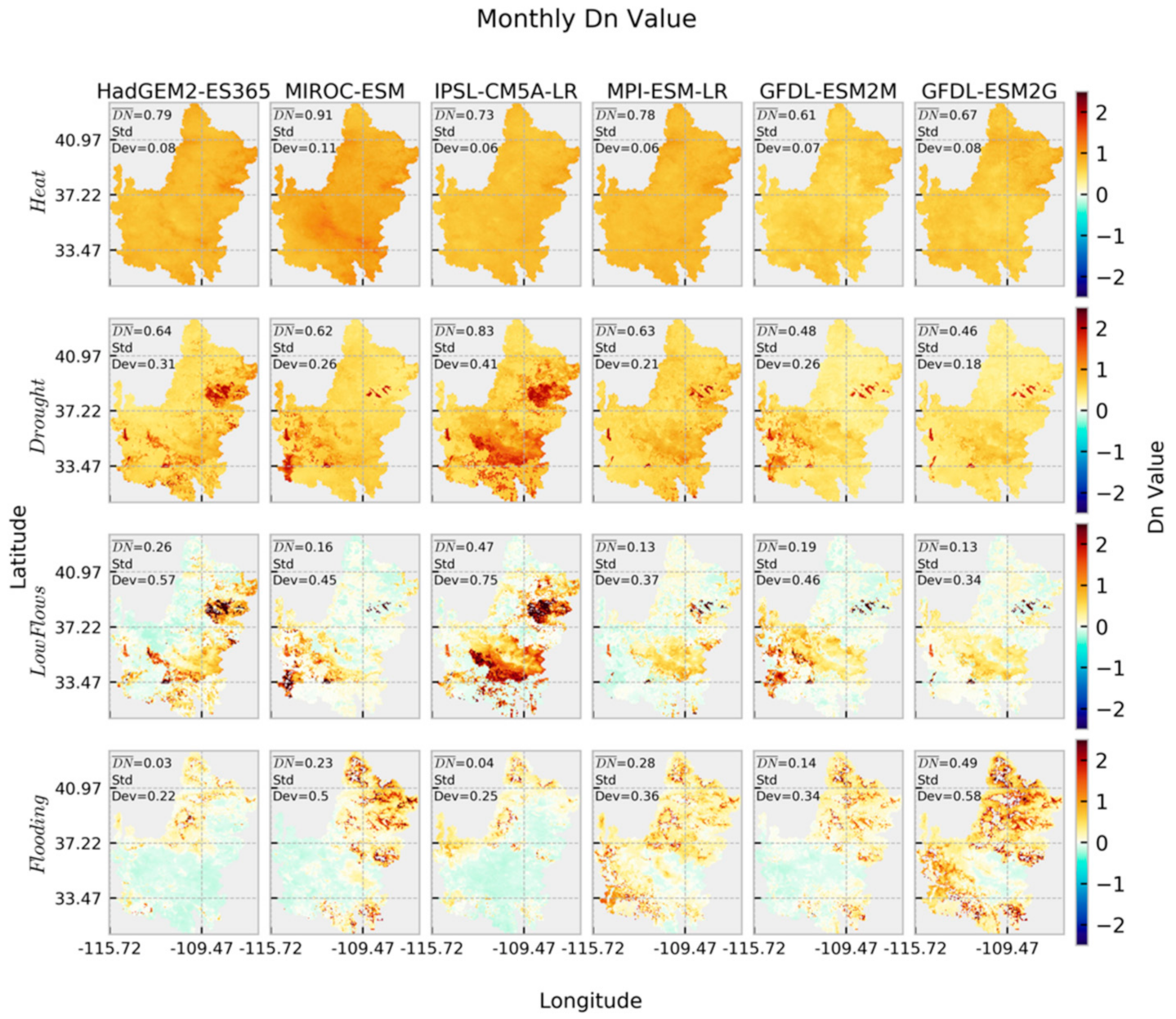
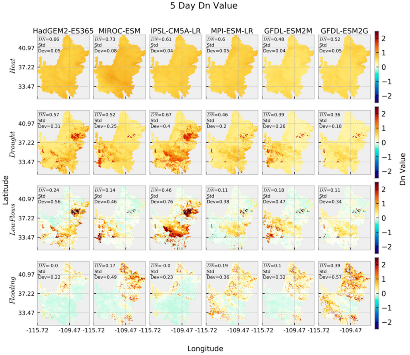
3. Results
3.1. Individual Indicators
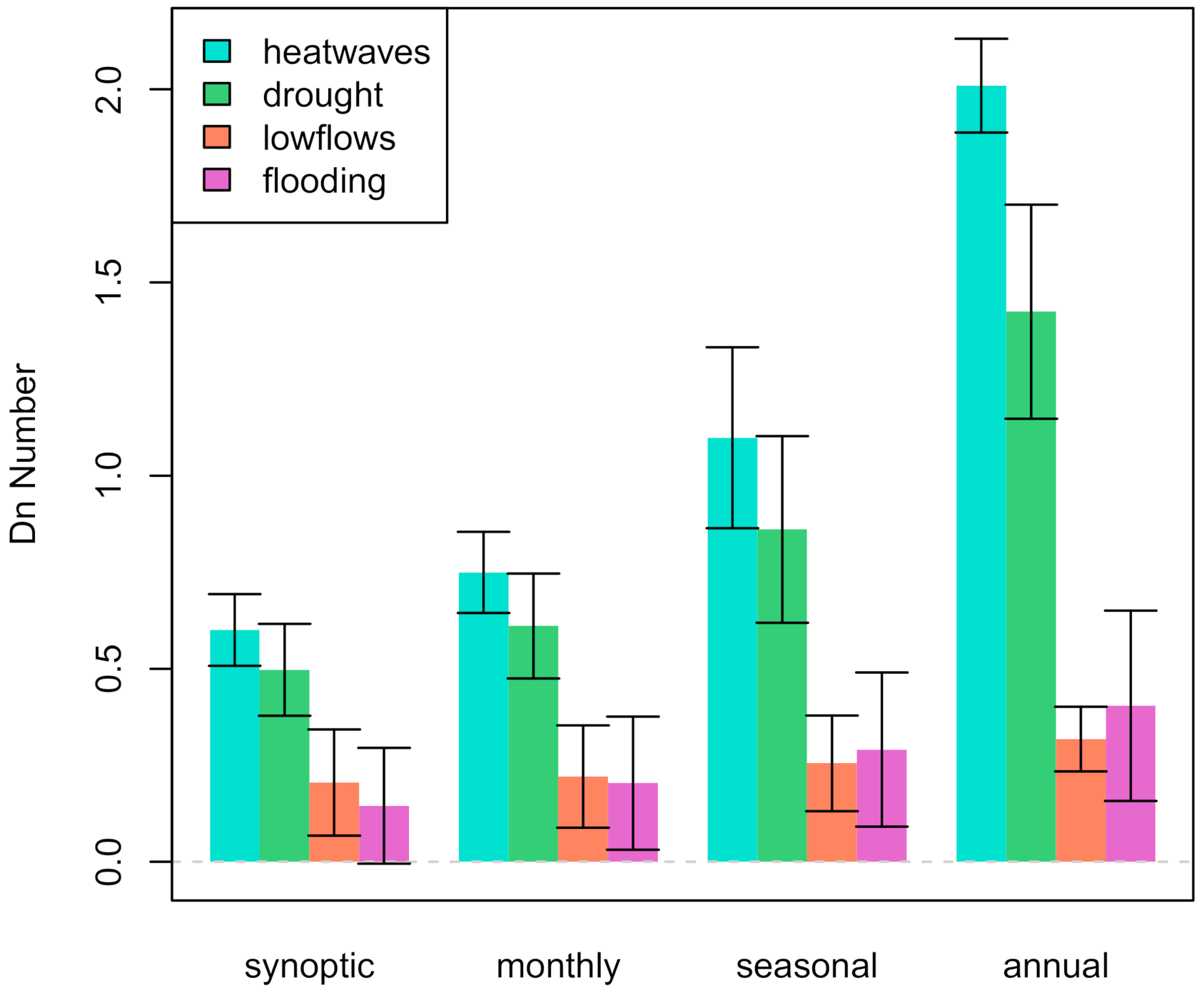
3.2. Impacts
4. Discussion
5. Conclusions
Author Contributions
Funding
Institutional Review Board Statement
Informed Consent Statement
Data Availability Statement
Acknowledgments
Conflicts of Interest
References
- NOAA. NOAA National Centers for Environmental Information (NCEI) U.S. Billion-Dollar Weather and Climate Disasters. 2021. Available online: https://www.ncdc.noaa.gov/billions/ (accessed on 30 March 2021).
- Stott, P. How climate change affects extreme weather events. Science 2016, 352, 1517–1518. [Google Scholar] [CrossRef]
- Chen, Y.; Moufouma-Okia, W.; Masson-Delmotte, V.; Zhai, P.; Pirani, A. Recent Progress and Emerging Topics on Weather and Climate Extremes Since the Fifth Assessment Report of the Intergovernmental Panel on Climate Change. Annu. Rev. Environ. Resour. 2018, 43, 35–59. [Google Scholar] [CrossRef]
- Trenberth, K.E.; Fasullo, J.T.; Shepherd, T.G. Attribution of climate extreme events. Nat. Clim. Chang. 2015, 5, 725–730. [Google Scholar] [CrossRef]
- National Academies of Sciences Engineering and Medicine. Attribution of Extreme Weather Events in the Context of Climate Change; National Academies Press: Washington, DC, USA, 2016. [Google Scholar] [CrossRef]
- Swain, D.L.; Singh, D.; Touma, D.; Diffenbaugh, N.S. Attributing extreme events to climate change: A new frontier in a warming world. One Earth 2020, 2, 522–527. [Google Scholar] [CrossRef]
- Field, C.B.; Barros, V.; Stocker, T.F.; Qin, D.; Dokken, D.J.; Ebi, K.L.; Mastrandrea, M.D.; Mach, K.J.; Plattner, G.-K.; Allen, S.K.; et al. Managing the Risks of Extreme Events and Disasters to Advance Climate Change Adaptation: Special Report of the Intergovernmental Panel on Climate Change; Cambridge University Press: Cambridge, UK; New York, NY, USA, 2012; p. 582. [Google Scholar]
- Blöschl, G.; Bierkens, M.F.; Chambel, A.; Cudennec, C.; Destouni, G.; Fiori, A.; Kirchner, J.W.; McDonnell, J.J.; Savenije, H.H.; Sivapalan, M. Twenty-three unsolved problems in hydrology (UPH)—A community perspective. Hydrol. Sci. J. 2019, 64, 1141–1158. [Google Scholar] [CrossRef]
- Fares, A.; Habibi, H.; Awal, R. Extreme events and climate change: A multidisciplinary approach. In Climate Change and Extreme Events; Elsevier: Amsterdam, The Netherlands, 2021; pp. 1–7. [Google Scholar]
- Driouech, F.; ElRhaz, K.; Moufouma-Okia, W.; Arjdal, K.; Balhane, S. Assessing future changes of climate extreme events in the CORDEX-MENA region using regional climate model ALADIN-climate. Earth Syst. Environ. 2020, 4, 477–492. [Google Scholar] [CrossRef]
- Bao, J.; Sherwood, S.C.; Alexander, L.V.; Evans, J.P. Future increases in extreme precipitation exceed observed scaling rates. Nat. Clim. Chang. 2017, 7, 128–132. [Google Scholar] [CrossRef]
- Maupin, M.A.; Ivahnenko, T.; Bruce, B. Estimates of Water Use and Trends in the Colorado River Basin, Southwestern United States, 1985–2010; Scientific Investigations Report 2018-5049; United States Geological Survey: Reston, VA, USA, 2018; p. 75.
- Broska, L.H.; Poganietz, W.-R.; Vögele, S. Extreme events defined—A conceptual discussion applying a complex systems approach. Futures 2020, 115, 102490. [Google Scholar] [CrossRef]
- McPhillips, L.E.; Chang, H.; Chester, M.V.; Depietri, Y.; Friedman, E.; Grimm, N.B.; Kominoski, J.S.; McPhearson, T.; Méndez-Lázaro, P.; Rosi, E.J.; et al. Defining Extreme Events: A Cross-Disciplinary Review. Earth Future 2018, 6, 441–455. [Google Scholar] [CrossRef]
- Sillmann, J.; Kharin, V.; Zhang, X.; Zwiers, F.; Bronaugh, D. Climate extremes indices in the CMIP5 multi-model ensemble. Part 1: Model evaluation in the present climate. J. Geophys. Res. Atmos. 2013. [Google Scholar] [CrossRef]
- Sillmann, J.; Kharin, V.; Zwiers, F.; Zhang, X.; Bronaugh, D. Climate extreme indices in the CMIP5 multi-model ensemble. Part 2: Future climate projections. J. Geophys. Res. Atmos. 2013, 118, 2473–2493. [Google Scholar] [CrossRef]
- Bennett, K.E.; Cannon, A.J.; Hinzman, L. Historical trends and extremes in boreal Alaska river basins. J. Hydrol. 2015, 527, 590–607. [Google Scholar] [CrossRef]
- Bennett, K.E.; Walsh, J. Spatial and temporal changes in indices of extreme precipitation and temperature for Alaska. Int. J. Climatol. 2015, 35, 1434–1452. [Google Scholar] [CrossRef]
- Tencer, B.; Weaver, A.; Zwiers, F. Joint occurrence of daily temperature and precipitation extreme events over Canada. J. Appl. Meteorol. Climatol. 2014, 53, 2148–2162. [Google Scholar] [CrossRef]
- Sadegh, M.; Moftakhari, H.; Gupta, H.V.; Ragno, E.; Mazdiyasni, O.; Sanders, B.; Matthew, R.; AghaKouchak, A. Multihazard scenarios for analysis of compound extreme events. Geophys. Res. Lett. 2018, 45, 5470–5480. [Google Scholar] [CrossRef]
- Tian, F.; Klingaman, N.P.; Dong, B. The driving processes of concurrent hot and dry extreme events in China. J. Clim. 2020. [Google Scholar] [CrossRef]
- Mazdiyasni, O.; AghaKouchak, A. Substantial increase in concurrent droughts and heatwaves in the United States. Proc. Natl. Acad. Sci. USA 2015, 112, 11484–11489. [Google Scholar] [CrossRef]
- Dowdy, A.J.; Catto, J.L. Extreme weather caused by concurrent cyclone, front and thunderstorm occurrences. Sci. Rep. 2017, 7, 40359. [Google Scholar] [CrossRef]
- Zhou, P.; Liu, Z. Likelihood of concurrent climate extremes and variations over China. Environ. Res. Lett. 2018, 13, 094023. [Google Scholar] [CrossRef]
- Zhou, S.; Williams, A.P.; Berg, A.M.; Cook, B.I.; Zhang, Y.; Hagemann, S.; Lorenz, R.; Seneviratne, S.I.; Gentine, P. Land-atmosphere feedbacks exacerbate concurrent soil drought and atmospheric aridity. Proc. Natl. Acad. Sci. USA 2019, 116, 18848–18853. [Google Scholar] [CrossRef]
- Hao, Z.; AghaKouchak, A.; Phillips, T.J. Changes in concurrent monthly precipitation and temperature extremes. Environ. Res. Lett. 2013, 8, 034014. [Google Scholar] [CrossRef]
- Toreti, A.; Cronie, O.; Zampieri, M. Concurrent climate extremes in the key wheat producing regions of the world. Sci. Rep. 2019, 9. [Google Scholar] [CrossRef]
- Kornhuber, K.; Coumou, D.; Vogel, E.; Lesk, C.; Donges, J.F.; Lehmann, J.; Horton, R.M. Amplified Rossby waves enhance risk of concurrent heatwaves in major breadbasket regions. Nat. Clim. Chang. 2020, 10, 48–53. [Google Scholar] [CrossRef]
- Beniston, M. Trends in joint quantiles of temperature and precipitation in Europe since 1901 and projected for 2100. Geophys. Res. Lett. 2009, 36. [Google Scholar] [CrossRef]
- Martin, J.-P.; Germain, D. Large-scale teleconnection patterns and synoptic climatology of major snow-avalanche winters in the Presidential Range (New Hampshire, USA). Int. J. Climatol. 2017, 37, 109–123. [Google Scholar] [CrossRef]
- Wazneh, H.; Arain, M.A.; Coulibaly, P.; Gachon, P. Evaluating the Dependence between Temperature and Precipitation to Better Estimate the Risks of Concurrent Extreme Weather Events. Adv. Meteorol. 2020, 2020, 8763631. [Google Scholar] [CrossRef]
- Luo, L.; Apps, D.; Arcand, S.; Xu, H.; Pan, M.; Hoerling, M. Contribution of temperature and precipitation anomalies to the California drought during 2012–2015. Geophys. Res. Lett. 2017, 44, 3184–3192. [Google Scholar] [CrossRef]
- Miao, C.; Sun, Q.; Duan, Q.; Wang, Y. Joint analysis of changes in temperature and precipitation on the Loess Plateau during the period 1961–2011. Clim. Dyn. 2016, 47, 3221–3234. [Google Scholar] [CrossRef]
- Fischer, E.M.; Knutti, R. Robust projections of combined humidity and temperature extremes. Nat. Clim. Chang. 2013, 3, 126–130. [Google Scholar] [CrossRef]
- Estrella, N.; Menzel, A. Recent and future climate extremes arising from changes to the bivariate distribution of temperature and precipitation in Bavaria, Germany. Int. J. Climatol. 2013, 33, 1687–1695. [Google Scholar] [CrossRef]
- AghaKouchak, A.; Cheng, L.; Mazdiyasni, O.; Farahmand, A. Global warming and changes in risk of concurrent climate extremes: Insights from the 2014 California drought. Geophys. Res. Lett. 2014, 41, 8847–8852. [Google Scholar] [CrossRef]
- Sedlmeier, K.; Feldmann, H.; Schädler, G. Compound summer temperature and precipitation extremes over central Europe. Theor. Appl. Climatol. 2018, 131, 1493–1501. [Google Scholar] [CrossRef]
- Sedlmeier, K.; Mieruch, S.; Schädler, G.; Kottmeier, C. Compound extremes in a changing climate—A Markov chain approach. Nonlinear Process. Geophys. 2016, 23, 375–390. [Google Scholar] [CrossRef]
- Hao, Z.; Singh, V.P. Drought characterization from a multivariate perspective: A review. J. Hydrol. 2015, 527, 668–678. [Google Scholar] [CrossRef]
- Hao, Z.; Singh, V.P.; Hao, F. Compound extremes in hydroclimatology: A review. Water 2018, 10, 718. [Google Scholar] [CrossRef]
- Beevers, L.; White, C.J.; Pregnolato, M. Editorial to the Special Issue: Impacts of Compound Hydrological Hazards or Extremes. Geosciences 2020, 10, 496. [Google Scholar] [CrossRef]
- Diffenbaugh, N.S.; Swain, D.L.; Touma, D. Anthropogenic warming has increased drought risk in California. Proc. Natl. Acad. Sci. USA 2015, 112, 3931–3936. [Google Scholar] [CrossRef]
- Raymond, C.; Horton, R.M.; Zscheischler, J.; Martius, O.; AghaKouchak, A.; Balch, J.; Bowen, S.G.; Camargo, S.J.; Hess, J.; Kornhuber, K.; et al. Understanding and managing connected extreme events. Nat. Clim. Chang. 2020, 10, 611–621. [Google Scholar] [CrossRef]
- Zscheischler, J.; Westra, S.; van den Hurk, B.J.J.M.; Seneviratne, S.I.; Ward, P.J.; Pitman, A.; AghaKouchak, A.; Bresch, D.N.; Leonard, M.; Wahl, T.; et al. Future climate risk from compound events. Nat. Clim. Chang. 2018, 8, 469–477. [Google Scholar] [CrossRef]
- Leonard, M.; Westra, S.; Phatak, A.; Lambert, M.; van den Hurk, B.; McInnes, K.; Risbey, J.; Schuster, S.; Jakob, D.; Stafford-Smith, M. A compound event framework for understanding extreme impacts. WIREs Clim. Chang. 2014, 5, 113–128. [Google Scholar] [CrossRef]
- Zscheischler, J.; Seneviratne, S.I. Dependence of drivers affects risks associated with compound events. Sci. Adv. 2017, 3, e1700263. [Google Scholar] [CrossRef]
- Livneh, B.; Bohn, T.J.; Pierce, D.W.; Munoz-Arriola, F.; Nijssen, B.; Vose, R.; Cayan, D.R.; Brekke, L. A spatially comprehensive, hydrometeorological data set for Mexico, the U.S., and Southern Canada 1950–2013. Sci. Data 2015, 2, 150042. [Google Scholar] [CrossRef]
- Christensen, N.S.; Lettenmaier, D.P. A multimodel ensemble approach to assessment of climate change impacts on the hydrology and water resources of the Colorado River Basin. Hydrol. Earth Syst. Sci. 2007, 11, 1417–1434. [Google Scholar] [CrossRef]
- Abatzoglou, J.T.; Brown, T.J. A comparison of statistical downscaling methods suited for wildfire applications. Int. J. Climatol. 2012, 32, 772–780. [Google Scholar] [CrossRef]
- Taylor, K.E.; Stouffer, R.J.; Meehl, G.A. An overview of CMIP5 and the experiment design. Bull. Am. Meteorol. Soc. 2012, 93, 485–498. [Google Scholar] [CrossRef]
- Collins, W.J.; Bellouin, N.; Doutriaux-Boucher, M.; Gedney, N.; Halloran, P.; Hinton, T.; Hughes, J.; Jones, C.D.; Joshi, M.; Liddicoat, S.; et al. Development and evaluation of an Earth-System model—HadGEM2. Geosci. Model Dev. 2011, 4, 1051–1075. [Google Scholar] [CrossRef]
- Cox, P.M. Description of the TRIFFID Dynamic Global Vegetation Model; Technical Note 24; Hadley Centre, United Kingdom Meteorological Office: Bracknell, UK, 2001.
- Sato, H.; Itoh, A.; Kohyama, T. SEIB-DGVM: A new Dynamic Global Vegetation Model using a spatially explicit individual-based approach. Ecol. Model. 2007, 200, 279–307. [Google Scholar] [CrossRef]
- Watanabe, S.; Hajima, T.; Sudo, K.; Nagashima, T.; Takcmura, T.; Okajima, H.; Nozawa, T.; Kawase, H.; Abe, M.; Yokohata, T. MIROC-ESM 2010: Model description and basic results of CMIP 5-20 c 3 m experiments. Geosci. Model Dev. 2011, 4, 845–872. [Google Scholar] [CrossRef]
- Giorgetta, M.A.; Jungclaus, J.; Reick, C.H.; Legutke, S.; Bader, J.; Böttinger, M.; Brovkin, V.; Crueger, T.; Esch, M.; Fieg, K. Climate and carbon cycle changes from 1850 to 2100 in MPI-ESM simulations for the Coupled Model Intercomparison Project phase 5. J. Adv. Model. Earth Syst. 2013, 5, 572–597. [Google Scholar] [CrossRef]
- Reick, C.; Raddatz, T.; Brovkin, V.; Gayler, V. Representation of natural and anthropogenic land cover change in MPI-ESM. J. Adv. Model. Earth Syst. 2013, 5, 459–482. [Google Scholar] [CrossRef]
- Krinner, G.; Viovy, N.; de Noblet-Ducoudré, N.; Ogée, J.; Polcher, J.; Friedlingstein, P.; Ciais, P.; Sitch, S.; Prentice, I.C. A dynamic global vegetation model for studies of the coupled atmosphere-biosphere system. Glob. Biogeochem. Cycles 2005, 19. [Google Scholar] [CrossRef]
- Dufresne, J.-L.; Foujols, M.-A.; Denvil, S.; Caubel, A.; Marti, O.; Aumont, O.; Balkanski, Y.; Bekki, S.; Bellenger, H.; Benshila, R. Climate change projections using the IPSL-CM5 Earth System Model: From CMIP3 to CMIP5. Clim. Dyn. 2013, 40, 2123–2165. [Google Scholar] [CrossRef]
- Shevliakova, E.; Pacala, S.W.; Malyshev, S.; Hurtt, G.C.; Milly, P.; Caspersen, J.P.; Sentman, L.T.; Fisk, J.P.; Wirth, C.; Crevoisier, C. Carbon cycling under 300 years of land use change: Importance of the secondary vegetation sink. Glob. Biogeochem. Cycles 2009, 23. [Google Scholar] [CrossRef]
- Delworth, T.L.; Broccoli, A.J.; Rosati, A.; Stouffer, R.J.; Balaji, V.; Beesley, J.A.; Cooke, W.F.; Dixon, K.W.; Dunne, J.; Dunne, K. GFDL’s CM2 global coupled climate models. Part I: Formulation and simulation characteristics. J. Clim. 2006, 19, 643–674. [Google Scholar] [CrossRef]
- Fajardo, J.; Corcoran, D.; Roehrdanz, P.R.; Hannah, L.; Marquet, P.A. GCM compareR: A web application to assess differences and assist in the selection of general circulation models for climate change research. Methods Ecol. Evol. 2020, 11, 656–663. [Google Scholar] [CrossRef]
- Le Quéré, C.; Moriarty, R.; Andrew, R.M.; Canadell, J.G.; Sitch, S.; Korsbakken, J.I.; Friedlingstein, P.; Peters, G.P.; Andres, R.J.; Boden, T. Global carbon budget 2015. Earth Syst. Sci. Data 2015, 7, 349–396. [Google Scholar] [CrossRef]
- Van Vuuren, D.P.; Edmonds, J.; Kainuma, M.; Riahi, K.; Thomson, A.; Hibbard, K.; Hurtt, G.C.; Kram, T.; Krey, V.; Lamarque, J.-F. The representative concentration pathways: An overview. Clim. Chang. 2011, 109, 5–31. [Google Scholar] [CrossRef]
- Bohn, T.J.; Vivoni, E.R. Process-based characterization of evapotranspiration sources over the North American monsoon region. Water Resour. Res. 2016, 52, 358–384. [Google Scholar] [CrossRef]
- Liang, X.; Lettenmaier, D.P.; Wood, E.F.; Burges, S.J. A simple hydrologically based model of land surface water and energy fluxes for general circulation models. J. Geophys. Res. 1994, 99, 14415–14428. [Google Scholar] [CrossRef]
- Franchini, M.; Pacciani, M. Comparative analysis of several conceptual rainfall-runoff models. J. Hydrol. 1991, 122, 161–219. [Google Scholar] [CrossRef]
- USBR. Colorado River Basin Natural Flow and Salt Data. Available online: https://www.usbr.gov/lc/region/g4000/NaturalFlow/supportNF.html (accessed on 24 December 2020).
- Yapo, P.O.; Gupta, H.V.; Sorooshian, S. Multi-objective global optimization for hydrologic models. J. Hydrol. 1998, 204, 83–97. [Google Scholar] [CrossRef]
- Bennett, K.E.; Bohn, T.J.; Solander, K.; McDowell, N.G.; Vivoni, E.; Middleton, R. Climate-driven disturbances in the San Juan River sub-basin of the Colorado River. Hydrol. Earth Syst. Sci. 2018, 22, 709–725. [Google Scholar] [CrossRef]
- Urrego-Blanco, J.R.; Hunke, E.C.; Urban, N.M.; Jeffery, N.; Turner, A.K.; Langenbrunner, J.R.; Booker, J.M. Validation of sea ice models using an uncertainty-based distance metric for multiple model variables. J. Geophys. Res. Ocean. 2017, 122, 2923–2944. [Google Scholar] [CrossRef]
- Langenbrunner, J.R.; Hemez, F.M.; Booker, J.M.; Ross, T.J. Model choice considerations and information integration using analytical hierarchy process. Procedia Soc. Behav. Sci. 2010, 2, 7700–7701. [Google Scholar] [CrossRef][Green Version]
- Booker, J.M. Interpretations of Langenbrunner’s Dn metric for V&V. In Los Alamos National Laboratory Technical Report; LA-UR-06-3720; Los Alamos National Laboratory: Los Alamos, NM, USA, 2006. [Google Scholar]
- IPCC. Climate Change 2013: The Physical Science Basis. Contribution of Working Group I to the Fifth Assessment Report of the Intergovernmental Panel on Climate Change (IPCC); Stocker, T., Qin, D., Plattner, G., Tignor, M., Allen, S., Boschung, J., Nauels, A., Xia, Y., Bex, B., Midgley, B., Eds.; Cambridge University Press: Cambridge, UK; New York, NY, USA, 2013; p. 1535. [Google Scholar]
- Omernik, J.M.; Griffith, G.E. Ecoregions of the conterminous United States: Evolution of a hierarchical spatial framework. Environ. Manag. 2014, 54, 1249–1266. [Google Scholar] [CrossRef]
- Hendricks, J.; Plescia, J. A review of the regional geophysics of the Arizona transition zone. J. Geophys. Res. Solid Earth 1991, 96, 12351–12373. [Google Scholar] [CrossRef]
- Sheppard, P.R.; Comrie, A.C.; Packin, G.D.; Angersbach, K.; Hughes, M.K. The climate of the US Southwest. Clim. Res. 2002, 21, 219–238. [Google Scholar] [CrossRef]
- Dirmeyer, P.A.; Schlosser, C.A.; Brubaker, K.L. Precipitation, recycling, and land memory: An integrated analysis. J. Hydrometeorol. 2009, 10, 278–288. [Google Scholar] [CrossRef]
- Garfin, G.; Franco, G.; Blanco, H.; Comrie, A.; Gonzalez, P.; Piechota, T.; Smyth, R.; Waskom, R. Southwest: The Third National Climate Assessment. In Climate Change Impacts in the United States: The Third National Climate Assessment; US Global Change Research Program: Washington, DC, USA, 2014; p. 25. [Google Scholar]
- Knutti, R.; Sedláček, J. Robustness and uncertainties in the new CMIP5 climate model projections. Nat. Clim. Chang. 2013, 3, 369–373. [Google Scholar] [CrossRef]
- Bennett, K.E.; Miller, G.; Talsma, C.; Jonko, A.; Bruggeman, A.; Atchley, A.; Lavadie-Bulnes, A.; Kwicklis, E.; Middleton, R. Future water resource shifts in the high desert Southwest of Northern New Mexico, USA. J. Hydrol. Reg. Stud. 2020, 28, 100678. [Google Scholar] [CrossRef]
- Frich, P.; Alexander, L.V.; Della-Marta, P.; Gleason, B.; Haylock, M.; Tank, A.K.; Peterson, T. Observed coherent changes in climatic extremes during the second half of the twentieth century. Clim. Res. 2002, 19, 193–212. [Google Scholar] [CrossRef]
- Livneh, B.; Hoerling, M.P. The physics of drought in the US central Great Plains. J. Clim. 2016, 29, 6783–6804. [Google Scholar] [CrossRef]
- Schoener, G.; Stone, M.C. Impact of antecedent soil moisture on runoff from a semiarid catchment. J. Hydrol. 2019, 569, 627–636. [Google Scholar] [CrossRef]
- Woldemeskel, F.; Sharma, A. Should flood regimes change in a warming climate? The role of antecedent moisture conditions. Geophys. Res. Lett. 2016, 43, 7556–7563. [Google Scholar] [CrossRef]
- Oubeidillah, A.; Tootle, G.; Piechota, T. Incorporating Antecedent Soil Moisture into Streamflow Forecasting. Hydrology 2019, 6, 50. [Google Scholar] [CrossRef]
- Castillo, V.; Gomez-Plaza, A.; Martınez-Mena, M. The role of antecedent soil water content in the runoff response of semiarid catchments: A simulation approach. J. Hydrol. 2003, 284, 114–130. [Google Scholar] [CrossRef]
- Tavakol, A.; Rahmani, V.; Harrington, J., Jr. Probability of compound climate extremes in a changing climate: A copula-based study of hot, dry, and windy events in the central United States. Environ. Res. Lett. 2020, 15, 104058. [Google Scholar] [CrossRef]
- Buma, B.; Livneh, B. Potential Effects of Forest Disturbances and Management on Water Resources in a Warmer Climate. For. Sci. 2015, 61, 895–903. [Google Scholar] [CrossRef]
- Vano, J.A.; Udall, B.; Cayan, D.R.; Overpeck, J.T.; Brekke, L.D.; Das, T.; Hartmann, H.C.; Hidalgo, H.G.; Hoerling, M.; McCabe, G.J. Understanding uncertainties in future Colorado River streamflow. Bull. Am. Meteorol. Soc. 2014, 95, 59–78. [Google Scholar] [CrossRef]
- Livneh, B.; Deems, J.S.; Buma, B.; Barsugli, J.J.; Schneider, D.; Molotch, N.P.; Wolter, K.; Wessman, C.A. Catchment response to bark beetle outbreak and dust-on-snow in the Colorado Rocky Mountains. J. Hydrol. 2015, 523, 196–210. [Google Scholar] [CrossRef]
- Hubbard, S.S.; Williams, K.H.; Agarwal, D.; Banfield, J.; Beller, H.; Bouskill, N.; Brodie, E.; Carroll, R.; Dafflon, B.; Dwivedi, D.; et al. The East River, Colorado, Watershed: A Mountainous Community Testbed for Improving Predictive Understanding of Multiscale Hydrological-Biogeochemical Dynamics. Vadose Zone J. 2018, 17, 180061. [Google Scholar] [CrossRef]
- Rivera, E.R.; Dominguez, F.; Castro, C.L. Atmospheric rivers and cool season extreme precipitation events in the Verde River basin of Arizona. J. Hydrometeorol. 2014, 15, 813–829. [Google Scholar] [CrossRef]
- House, P.K.; Hirschboeck, K.K. Hydroclimatological and paleohydrological context of extreme winter flooding in Arizona, 1993. In Storm-Induced Geological Hazards: Case Histories from the 1992–1993 Winter Storm in Southern California and Arizona. Reviews in Engineering Geology; Larson, R.A., Slosso, J.E., Eds.; Geological Society of America: Boulder, CO, USA, 1997; Volume 11, pp. 1–24. [Google Scholar]
- US Army Corps of Engineers. Flood Damage Report, State of Arizona, Floods of 1993; US Army Corps of Engineers: Los Angeles, CA, USA, 1994; p. 107. [Google Scholar]
- Kopytkovskiy, M.; Geza, M.; McCray, J. Climate-change impacts on water resources and hydropower potential in the Upper Colorado River Basin. J. Hydrol. Reg. Stud. 2015, 3, 473–493. [Google Scholar] [CrossRef]
- Molotch, N.P.; Fassnacht, S.R.; Bales, R.C.; Helfrich, S.R. Estimating the distribution of snow water equivalent and snow extent beneath cloud cover in the Salt-Verde River basin, Arizona. Hydrol. Process. 2004, 18, 1595–1611. [Google Scholar] [CrossRef]
- Rahmstorf, S.; Coumou, D. Increase of extreme events in a warming world. Proc. Natl. Acad. Sci. USA 2011, 108, 17905–17909. [Google Scholar] [CrossRef]


| Indicators | Description and Units | Abbreviation |
|---|---|---|
| Maximum temperature | Maximum temperature achieved over the time period (°C) | tx |
| Maximum precipitation | Maximum daily precipitation over the time period (mm) | precx |
| Low precipitation days | Number of days when accumulated precipitation is <0.01 mm. (count) | dryd |
| Maximum streamflow | Maximum daily streamflow over the time period (mm) | qx |
| Minimum streamflow | Minimum daily streamflow over the time period(mm) | qn |
| Maximum soil moisture | Maximum daily soil moisture from the third soil moisture layer over the time period (mm) | soilmx |
| Minimum soil moisture | Minimum daily soil moisture from the third soil moisture layer over the time period (mm) | soilmn |
| Maximum evapotranspiration (ET) | Maximum daily evapotranspiration over the time period (mm) | evapx |
| Impacts | Indicators |
|---|---|
| Heat Waves | Maximum temperature, maximum ET |
| Drought | Maximum temperature, low precipitation days, minimum soil moisture |
| Low Flows | Minimum streamflow, minimum soil moisture, maximum ET |
| Flooding | Maximum precipitation, maximum streamflow, maximum soil moisture |
| Historical | Future | Change | ||||
|---|---|---|---|---|---|---|
| Temp. (°C) | Precip. (mm) | Temp. (°C) | Precip. (mm) | Temp. (°C) | Precip. (mm) | |
| GFDL-ESM2G | 11.7 | 365.9 | 16.3 | 403 | 4.5 | 37.2 |
| GFDL-ESM2M | 11.7 | 366.5 | 15.8 | 377.9 | 4.1 | 11.3 |
| HadGEM2-ES365 | 11.8 | 366.8 | 18 | 360.4 | 6.2 | −6.4 |
| IPSL-CM5A-LR | 11.9 | 351.7 | 18.2 | 298.9 | 6.3 | −52.8 |
| MIROC-ESM | 11.8 | 369.9 | 18.8 | 400.7 | 7 | 30.8 |
| MPI-ESM-LR | 11.9 | 363.5 | 17 | 356.3 | 5.1 | −7.3 |
| Average | 11.8 | 364.1 | 17.3 | 366.2 | 5.5 | 2.1 |
| Standard Deviation | 0.1 | 6.4 | 1.2 | 38.3 | 1.2 | 32.6 |
| Synoptic | Monthly | Seasonal | Annual | ||
|---|---|---|---|---|---|
| CRB | Heatwaves | 0.60 (0.09) | 0.75 (0.11) | 1.10 (0.23) | 2.01 (0.12) |
| Drought | 0.50 (0.12) | 0.61 (0.14) | 0.86 (0.24) | 1.42 (0.28) | |
| Low Flows | 0.21 (0.14) | 0.22 (0.13) | 0.26 (0.12) | 0.32 (0.08) | |
| Flooding | 0.14 (0.15) | 0.20 (0.17) | 0.29 (0.20) | 0.40 (0.25) | |
| Upper CRB | Heatwaves | 0.60 (0.08) | 0.75 (0.10) | 1.11 (0.19) | 2.02 (0.13) |
| Drought | 0.44 (0.13) | 0.55 (0.15) | 0.79 (0.25) | 1.35 (0.29) | |
| Low Flows | 0.14 (0.15) | 0.15 (0.15) | 0.19 (0.15) | 0.27 (0.14) | |
| Flooding | 0.27 (0.20) | 0.34 (0.22) | 0.44 (0.24) | 0.60 (0.29) | |
| Lower CRB | Heatwaves | 0.60 (0.10) | 0.75 (0.12) | 1.09 (0.27) | 2.00 (0.14) |
| Drought | 0.55 (0.12) | 0.66 (0.14) | 0.92 (0.25) | 1.49 (0.28) | |
| Low Flows | 0.27 (0.15) | 0.28 (0.14) | 0.31 (0.13) | 0.36 (0.08) | |
| Flooding | 0.04 (0.12) | 0.09 (0.15) | 0.16 (0.18) | 0.24 (0.23) |
Publisher’s Note: MDPI stays neutral with regard to jurisdictional claims in published maps and institutional affiliations. |
© 2021 by the authors. Licensee MDPI, Basel, Switzerland. This article is an open access article distributed under the terms and conditions of the Creative Commons Attribution (CC BY) license (https://creativecommons.org/licenses/by/4.0/).
Share and Cite
Bennett, K.E.; Talsma, C.; Boero, R. Concurrent Changes in Extreme Hydroclimate Events in the Colorado River Basin. Water 2021, 13, 978. https://doi.org/10.3390/w13070978
Bennett KE, Talsma C, Boero R. Concurrent Changes in Extreme Hydroclimate Events in the Colorado River Basin. Water. 2021; 13(7):978. https://doi.org/10.3390/w13070978
Chicago/Turabian StyleBennett, Katrina E., Carl Talsma, and Riccardo Boero. 2021. "Concurrent Changes in Extreme Hydroclimate Events in the Colorado River Basin" Water 13, no. 7: 978. https://doi.org/10.3390/w13070978
APA StyleBennett, K. E., Talsma, C., & Boero, R. (2021). Concurrent Changes in Extreme Hydroclimate Events in the Colorado River Basin. Water, 13(7), 978. https://doi.org/10.3390/w13070978