Article

Relative Performance of 1-D Versus 3-D Hydrodynamic, Water-Quality Models for Predicting Water Temperature and Oxygen in a Shallow, Eutrophic, Managed Reservoir

1
Centre for Wind, Waves and Water, School of Civil Engineering, The University of Sydney, Sydney, NSW 2006, Australia
2
Department of Biological Sciences, Virginia Polytechnic Institute and State University, 2025 Derring Hall, Virginia Tech, Blacksburg, VA 24061, USA
3
Department of Civil and Environmental Engineering, Virginia Polytechnic Institute and State University, 401 Durham Hall, Virginia Tech, Blacksburg, VA 24061, USA
*
Author to whom correspondence should be addressed.
Water 2021, 13(1), 88; https://doi.org/10.3390/w13010088
Submission received: 28 November 2020 / Revised: 26 December 2020 / Accepted: 28 December 2020 / Published: 3 January 2021
(This article belongs to the Special Issue Physical Processes in Lakes)

Abstract

:
Many researchers use one-dimensional (1-D) and three-dimensional (3-D) coupled hydrodynamic and water-quality models to simulate water quality dynamics, but direct comparison of their relative performance is rare. Such comparisons may quantify their relative advantages, which can inform best practices. In this study, we compare two 1-year simulations in a shallow, eutrophic, managed reservoir using a community-developed 1-D model and a 3-D model coupled with the same water-quality model library based on multiple evaluation criteria. In addition, a verified bubble plume model is coupled with the 1-D and 3-D models to simulate the water temperature in four epilimnion mixing periods to further quantify the relative performance of the 1-D and 3-D models. Based on the present investigation, adopting a 1-D water-quality model to calibrate a 3-D model is time-efficient and can produce reasonable results; 3-D models are recommended for simulating thermal stratification and management interventions, whereas 1-D models may be more appropriate for simpler model setups, especially if field data needed for 3-D modeling are lacking.

1. Introduction

One-dimensional (1-D) coupled hydrodynamic models, which simulate water balance and thermal stratification dynamics in lake and reservoir ecosystems [1,2], are popular due to their low computational requirements. Linked with biogeochemical and ecological modeling libraries, their computational efficiency allows 1-D models to quickly simulate vertical stratification in lake dynamics [3,4] including oxygen and long-term nutrient cycles [5,6]. Verified against field data using metrics such as root mean square error (RMSE) and normalized mean absolute error (NMAE) [7], 1-D models have been adopted to simulate water-quality variables such as dissolved oxygen (DO) and nutrient concentrations with adequate accuracy in many water bodies [8,9,10].
In contrast, three-dimensional (3-D) coupled hydrodynamic models are necessary to simulate spatially-resolved hydrodynamic and water-quality variables including oxygen [11,12] and plankton [13], especially in large aquatic ecosystems and the ocean [14,15,16]. Further, 3-D models may be particularly useful in waterbodies with complex bathymetry or that experience dynamic conditions [
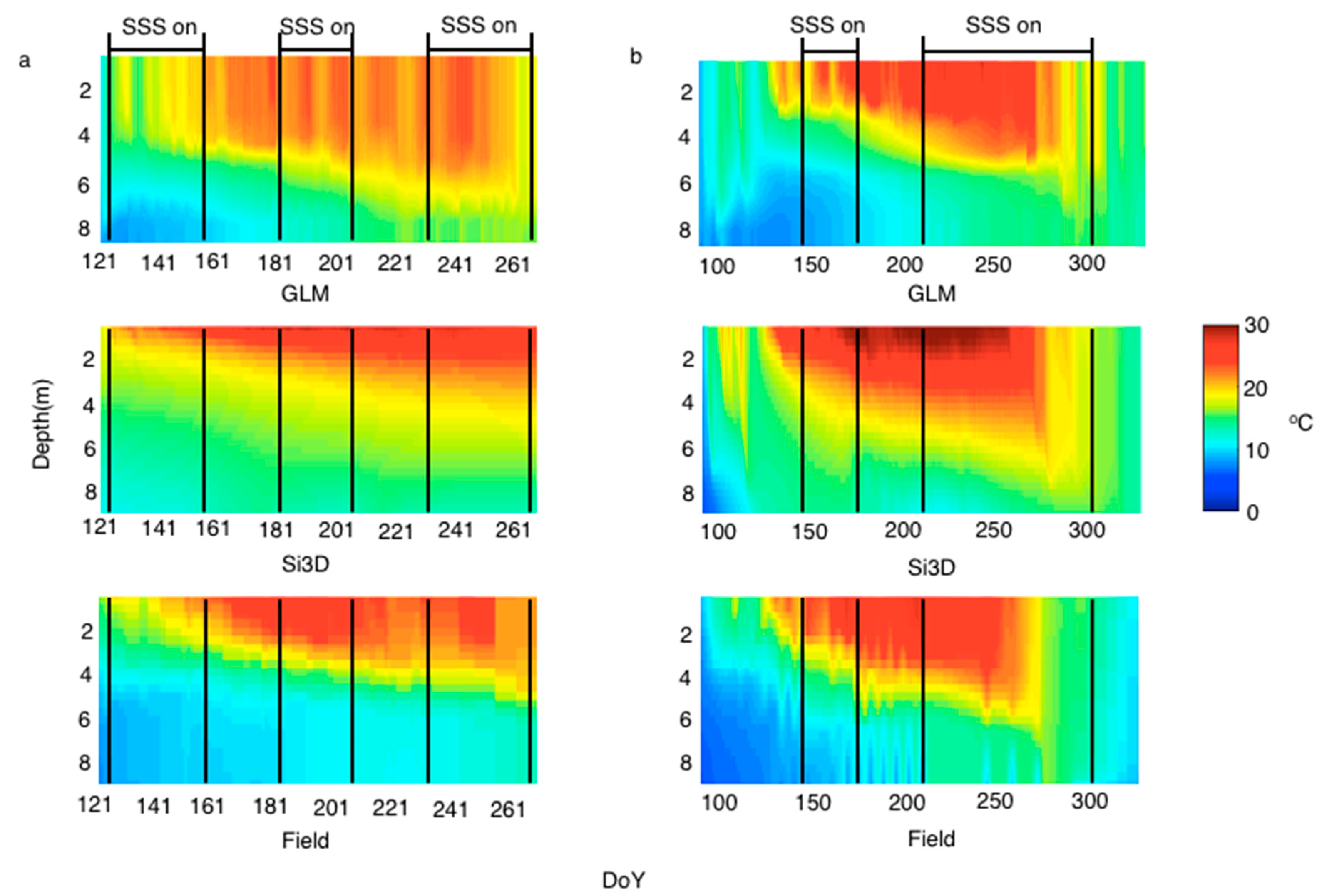
17]. For example, 3-D coupled hydrodynamic and water-quality models are useful for lake and reservoir management when engineered systems, including side steam supersaturation (SSS) and epilimnion mixing (EM), are installed to improve water quality [18,19]. One common perception [20] is that 3-D models are better in simulating engineered water bodies.
A direct comparison of the modeling results of 1-D and 3-D models may reveal the relative advantages of the different models in a quantitative manner. Fleischmann et al. [21] studied trade-offs between 1-D and 2-D regional river hydrodynamic models, but a similar study is absent in existing lake and reservoir research for 1-D and 3-D models. In addition, in certain situations, concurrent adoption of both 1-D and 3-D models may be needed to achieve simulation goals because of their complementary benefits.
One example of concurrent adoption of both 1-D and 3-D models is Romero et al. [22], who used a 3-D coupled hydrodynamic and aquatic ecological model to simulate a flood underflow through Lake Burragorang, a deep lake near Sydney, Australia. Due to the flood underflow, biogeochemical distributions varied spatially and temporally, which could not be captured by the 1-D model. At the same time, their team used a 1-D coupled hydrodynamic and aquatic ecological model to simulate Lake Burragorang for over two years due to the low computational needs for long-term calibration and validation of 1-D models. In this case, quantifying the relative advantages of the 1-D and 3-D models are crucial for obtaining reliable simulation results in a timely manner.
Romero et al. [22] also found that one set of biogeochemical parameters can be adopted in both 1-D and 3-D models to adequately simulate nutrient and plankton dynamics in the lake, which provides another reason for concurrent adoption of both 1-D and 3-D models. Parameter identification and sensitivity analysis are critical for performance evaluation when using ecological modeling libraries linked with hydrodynamic models [23], usually requiring thousands of repeated model runs. This is feasible with 1-D models due to their high computational efficiency. However, it is extremely time-consuming to do the same with 3-D models, for which a single one-year simulation may take up to a few days of real time even on high-performance computer clusters. Since most ecological parameters in 3-D models are chosen based on literature values or manual tuning, using 1-D models as a test-bed may be an efficient solution for parameter identification and sensitivity analysis for 3-D models.
Similar to the work carried out by Romero et al. [22], this study adopts a 1-D model as a test-bed environment to speed up the calibration of a 3-D hydrodynamic and water-quality model. Further, this study employs well-calibrated biogeochemical parameters of a 1-D coupled hydrodynamic and water-quality model in a 3-D model of a shallow eutrophic reservoir.
When performing numerical simulations, both the spatial and temporal resolutions may affect the numerical accuracy. Reducing spatial and temporal resolutions shortens computing time. However, a lower temporal resolution may lead to errors in energy balance [24], and a lower spatial resolution may fail to resolve the bathymetry of water bodies [25]. Therefore, it is necessary to compromise between the numerical accuracy and the computational efficiency when determining the spatial and temporal resolutions. Numerical tests are performed to determine a suitable cell size for calibration and simulation.
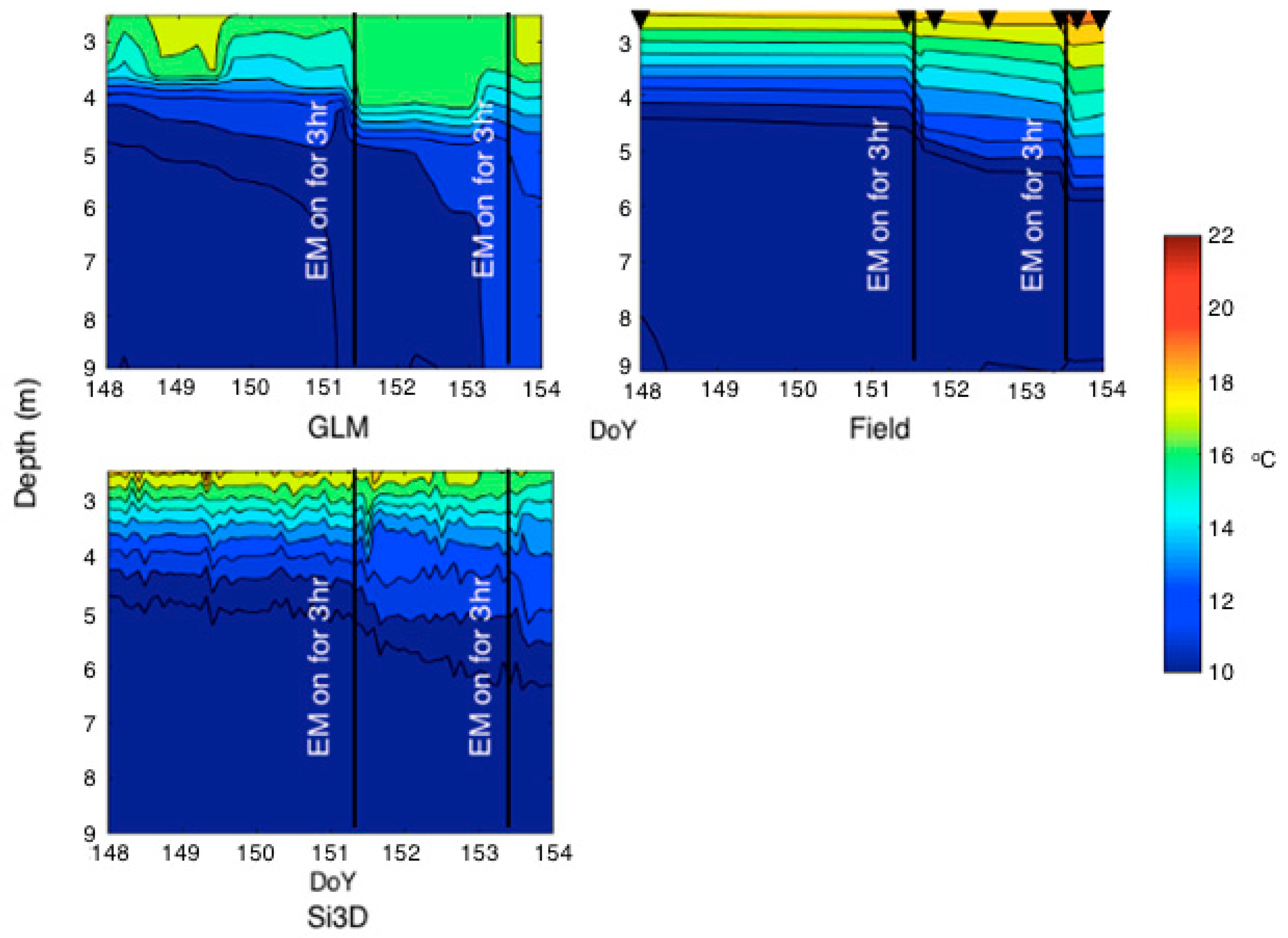
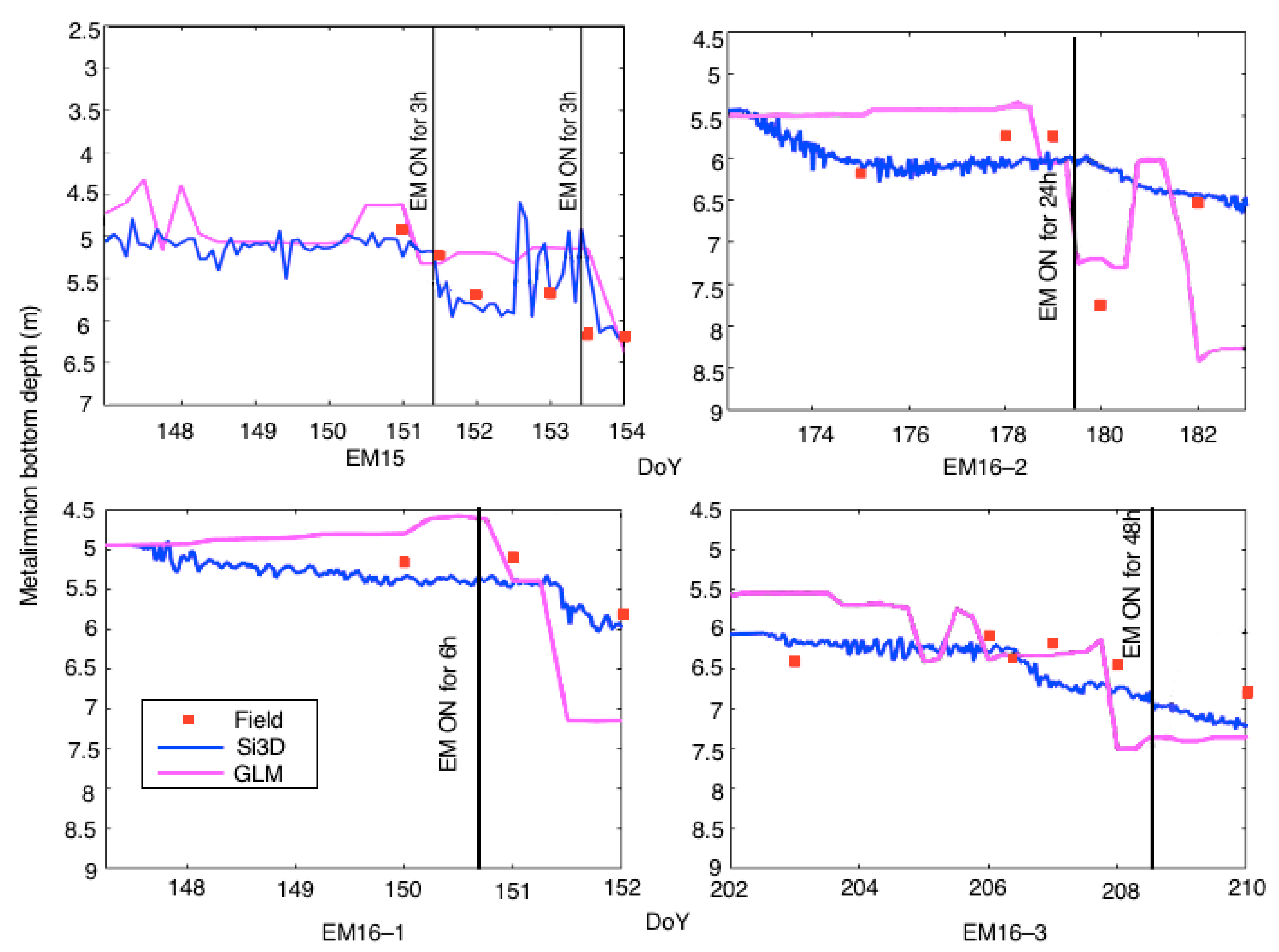
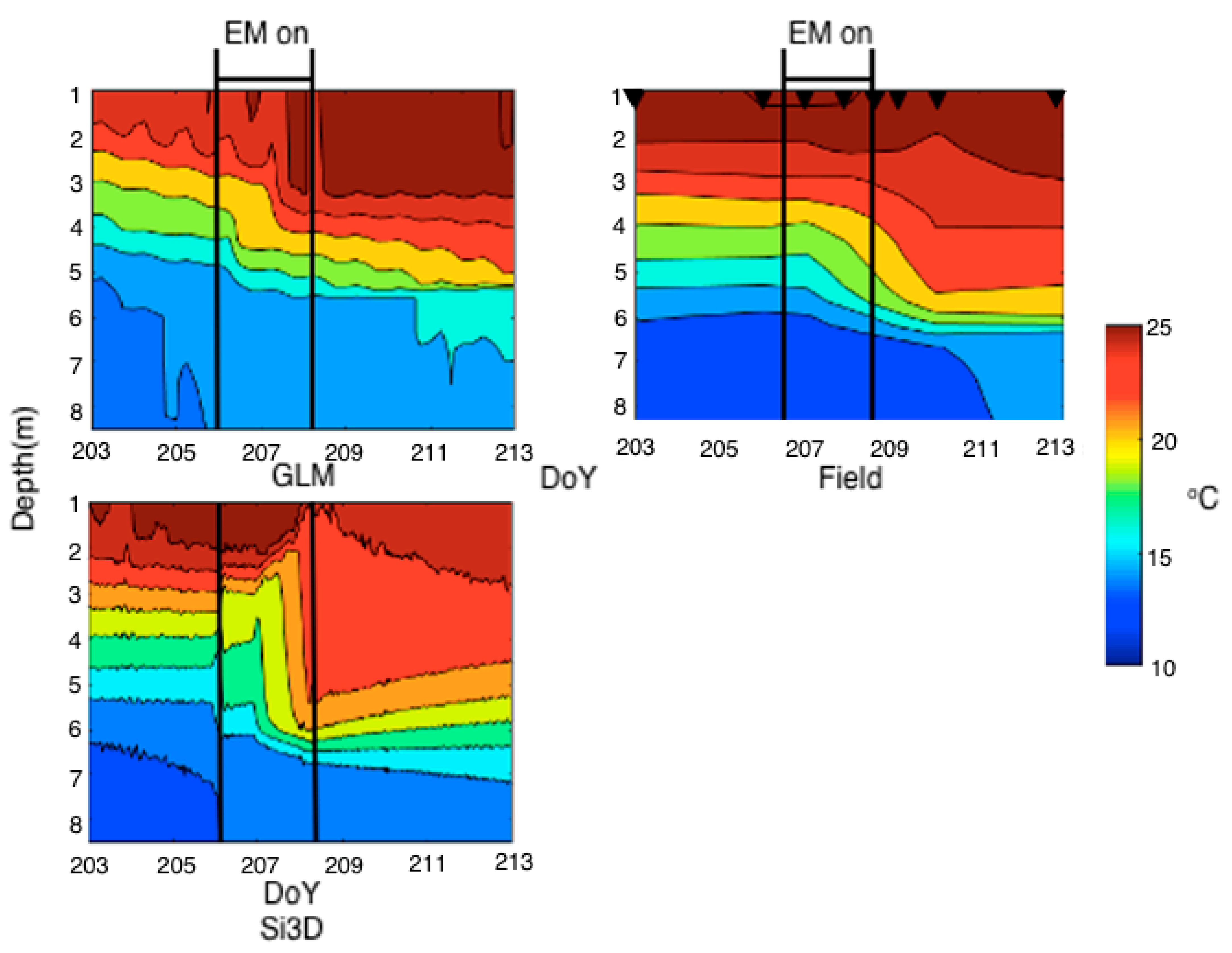
Temperature and DO field data collected over two one-year periods are used to verify the simulation results. The aim of this study is to quantify the relative advantages of 1-D and 3-D coupled hydrodynamic and water-quality models and determine the most time-efficient modeling approach with combined 1-D and 3-D calibration and modeling. In addition, this study is the first attempt to implement 1-D EM modeling, with two bubble plume model variants enabled in the 1-D and 3-D coupled models. Additional simulations of four EM periods over two years are carried out to compare the two bubble plume models and the 1-D and 3-D EM modeling approaches.

2. Study Methods

2.1. Study Sites and Artificial Mixing Systems

The study site is Falling Creek Reservoir (FCR) (Figure 1) in Virginia, USA (37°18′20″ N, 79°50′19″ W), a eutrophic, shallow, drinking-water reservoir managed by Western Virginia Water Authority (WVWA). Persistent hypolimnetic hypoxia and occasional algae blooms have caused water-quality problems in FCR during the stratified period [26,27], which shorten filter run times and increase soluble iron, manganese and phosphorus released from the sediment.
FCR is equipped with a side-stream supersaturation system and an epilimnion mixing system to address these concerns. The SSS system consists of a submersible pump, inlet piping, oxygen source, oxygen contact chamber, outlet piping and distribution header with nozzles [28]. The EM system consists of a compressed air system on land and a distribution header submerged in the water [29]. The SSS system aims to add DO to the hypolimnion, while the EM system is designed to inject air to mix and deepen the surface mixed layer above the hypolimnion, thereby hindering the growth of algae [29,30]. The SSS distribution header is positioned 1 m above the sediment in the hypolimnion, while the EM diffuser is located approximately 5 m below the water surface.
Field data was collected in FCR continuously over 5 years from 2013 to 2018. Figure 1 presents the locations of the SSS distribution header, the EM diffuser and the five locations (FCR10, FCR20, FCR30, FCR45 and FCR50) where data were collected. FCR50 is at the deepest point near the intake of the water treatment plant.
The collected field data included water temperature, DO and meteorological data. An SBE 19 plus high-resolution (4 Hz sampling rate) conductivity, temperature, and depth (CTD) profiler customized with an SBE 43 DO probe (Seabird Electronics, Bellevue, WA, USA) and a ProODO meter (YSI Inc., Yellow Springs, OH, USA) was used to collect depth profiles of the temperature and DO. The CTD can collect data at 0.1 m increments in the water column with a response time of 1.4 s at 20 °C, and the ProODO meter was used to check the quality of the temperature and DO data collected by the CTD. The hourly meteorological data required for the numerical modeling were obtained from North American Land Assimilation System-2 (NLDAS-2) project (https://ldas.gsfc.nasa.gov/nldas/v2/models).
Table 1 shows the details of the field campaign, simulation periods and oxygenation settings for 2014 and 2015, and Table 2 presents the simulation dates of Si3D-AED2 and GLM-AED2, the EM operation periods and the corresponding flow rates in the years 2015 and 2016.

2.2. The 1-D Model

To simulate freshwater systems at a global scale [31], the General Lake Model (GLM) was developed as a community 1-D hydrodynamic model for enclosed aquatic systems [32]. The open source model has been applied to natural and managed systems from wetlands and ponds to deep lakes with diverse climate conditions [33,34]. With continuous development of the GLM software and a growing modeling community, an increasing number of data visualization and processing tools are available for GLM [35,36].
GLM adopts a 1-D approach that resolves a series of horizontal layers [32], with core layer and mixing algorithms similar to the dynamic reservoir simulation model (DYRESM) [1] and the dynamic lake model (DLM) [37]. This approach defines each layer as a ‘control volume’ that can contract or expand in response to inflows/outflows and mixing with adjacent layers. The model solves the water balance in the lake domain, where the layers amalgamate, expand, contract or split due to water density changes caused by surface heating, vertical mixing and inflows/outflows. Regarding the energy balance approach, GLM estimates the amount of turbulent kinetic energy available for the surface mixed layer (surface mixing) and layers below the thermocline (deep mixing) respectively to simulate mixing dynamics. For surface mixing, the deepening rate of the surface mixed layer is calculated based on the balance between the available turbulent kinetic energy and the energy required for mixing to occur. The deep mixing is modeled using a characteristic vertical diffusivity, which is either approximated as a constant or using an equation introduced by Weinstock [38]. The vertical diffusivity is used to estimate the diffusion of scalars (including temperature and water-quality variables) between two neighboring layers.
Each layer also contains heat and other constituents, generally referred to as scalars. The scalars are conserved when layers change thickness or merge/split. The heat budget of the surface layer is determined by a balance of shortwave and longwave radiation fluxes as well as sensible and latent heat fluxes. In addition, a sediment heat module is available in GLM for modeling the heat exchange between the sediment and the water column. When the module is turned on, each water layer changes its temperature at a rate depending on the area in contact with the sediment and the local temperature gradient, as described by Hipsey et al. [32].
As already mentioned, coupled models are used to simulate the operation of the SSS and EM systems. GLM can include submerged inflows at any user-specified depth, which is used to simulate the SSS in FCR in the present investigation. The oxygenated water is first extracted then added to FCR at 8 m depth as a new layer.
A bubble plume module is enabled in GLM [39] to simulate epilimnion mixing. In this study, two variants of the bubble plume model are tested for GLM: the first bubble plume model detrains the entrained water at the depth of neutral buoyancy (GLM_DNB), and the second model detrains the entrained water at the depth of maximum plume rise (GLM_DMPR). The results of these two models are compared to determine which detrainment option simulates bubble plume mixing better in GLM, as described in Section 3 and Section S4 of Supplementary Materials.
GLM is pre-linked with the aquatic ecodynamic model (AED2) library to resolve the vertical profiles of water-quality variables of interest (such as oxygen, methane, etc.) [32]. GLM-AED2 was calibrated with field data collected over the period of 2013–2018 using manual adjustments and auto-calibrating scripts. The hydrodynamic model (GLM) was calibrated using Markov-chain Monte Carlo (MCMC) [40] tools, and the water-quality model (AED2) was calibrated by covariance matrix adaptation evolution strategy (CMA-ES) [41]. The version of GLM used in this study is 3.0.0 beta 10, and the version of AED2 is 1.3.4.

2.3. The 3-D Model

Si3D is a 3-D hydrodynamic model, which adopts a finite-difference method to obtain numerical solutions of the Navier–Stokes equations [42]. Si3D and its coupled models for simulating artificial mixing have been validated in previous studies of oxygenated reservoirs [12,43]. A coupled water-jet model with Si3D has been verified with field temperature data in FCR during oxygenation period [20]. The water-jet model accounts for both the momentum induced by the jet discharge and the ambient flow entrained by the expanding jet to resolve the small-scale jet flow within larger grid cells.
Details of the coupled bubble plume model with Si3D can be found in the literature [12,39], which has been verified for Spring Hollow Reservoir, VA, USA by Singleton et al. [12] and for FCR by Chen et al. [20]. Similar to the bubble plume models coupled with GLM, the bubble plume model in Si3D includes entrainment of ambient water and detrainment when the bubble-plume system is in operation. In this study, two variants of bubble plume models are tested for Si3D and the following acronyms are used to differentiate these two bubble plume models: Si3D_DNB for the plume model detraining the entrained water at the depth of neutral buoyancy; and Si3D_DMPR for the plume model detraining the entrained water at the depth of maximum plume rise (DMPR).
Si3D was coupled with AED2 through the Framework of Aquatic Biogeochemistry Model Library (FABM) [44]. FABM acts as an interface between the hydrodynamic host model (Si3D) and the coupled biogeochemical model (AED2). At each time-step, FABM first refers physical data (e.g., temperature, pressure) and tracer states (e.g., oxygen, phytoplankton) from the hydrodynamic host model to the coupled biogeochemical model, then the ecological variables (e.g., oxygen, phytoplankton) modelled by the biogeochemical model are returned to the hydrodynamic host model as biogeochemical source-sink terms [29]. With this coupling, the modules in AED2 can interactively simulate a range of water-quality variables of interest, including DO and sediment flux. The version of AED2 library coupled with Si3D is 1.3.4.

3. Numerical Tests

To determine appropriate spatial and temporal resolutions for the 1-D and 3-D models, GLM-AED2 time-step dependence test and Si3D-AED2 grid and time-step dependence tests are carried out.
In the existing studies using 1-D models including GLM, hourly time-steps are usually adopted [32]. These studies have demonstrated the capability of the 1-D models for correctly simulating water body temperature using hourly time-steps, confirming the high computational efficiency of the 1-D models. However, no GLM-AED2 time-step dependence test has been reported to reveal how model performance varies with the time-step. The purpose of the time-step dependence test is to examine the impact of the time-step on the simulated lake thermal structure. A number of time-steps ranging from one hour to one day are tested. Time-steps shorter than one hour are not tested here since the time resolution of meteorological data is one hour. These test runs with different time-steps simulate the temperature variation in FCR from 31 March (day of year—DoY 90) to 31 July (DoY 212) in 2015 without inflow/outflow and oxygenation. The details of the tested time-steps and the corresponding test results are presented in Section S1 of Supplementary Materials. Based on the time-step dependence test, the 3600 s time-step is adopted for the subsequent GLM-AED2 model runs due to its good compromise between the computational efficiency and numerical accuracy.
The sensitivity of the 3-D modeling results to the grid resolution and time-step is also examined to determine a suitable grid resolution and time-step setting for subsequent calculations. Starting with a relatively coarse grid of 10 m × 40 m × 0.6 m and a relatively large time-step of 10 s, the grid is refined twice by halving the cell sizes and in the meantime, the time-step is also halved twice to keep the CFL (Courant–Freidrich–Lewy) number [45] the same among the three sets of calculations. The tests run with the different cell sizes and time-steps calculate the temperature and DO in FCR using Si3D-AED2 over the period of 31 March (DoY 90) to 27 November (DoY 331) in 2015 without inflow/outflow and oxygenation. Further details of the test settings and the corresponding results are presented in 
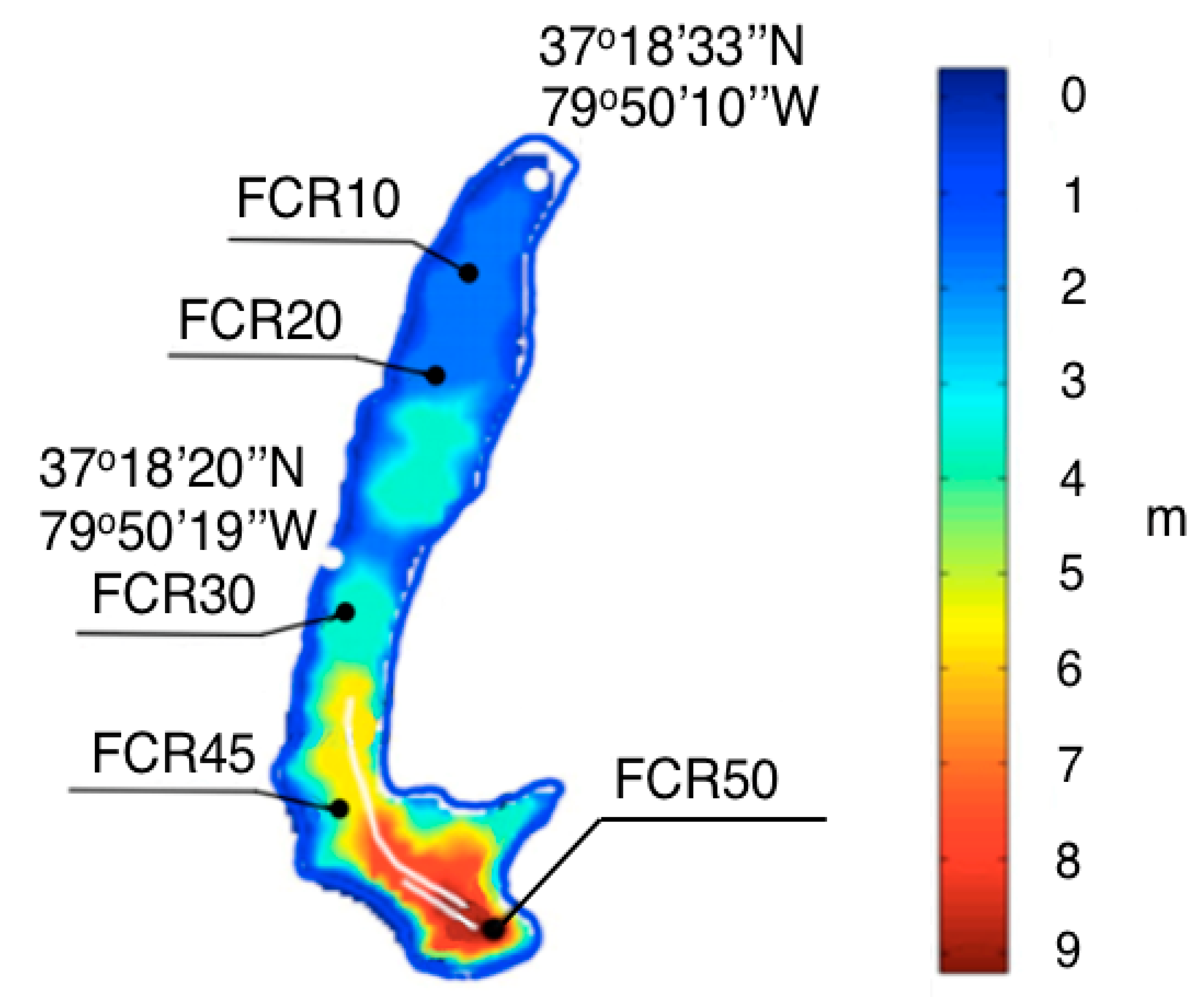
Section S2 of Supplementary Materials. Based on these test results, the 5 m × 20 m × 0.3 m cell size is adopted for subsequent Si3D-AED2 simulations to ensure good accuracy in both stratified and mixed periods. Here, the time period between the spring and fall turnover is referred to as the stratified period, and the rest of the year is referred to as the mixed period. Spring and fall turnover is defined as the days when the temperature at 1 m equals the temperature at 8 m using observations made every 15 min throughout the monitoring period by two optical INW DO2 DO sondes (Seametrics, WA, USA) [46].
In addition to the dependence on the spatial and temporal resolutions, different model configurations may also affect the numerical results. The sediment heat module is an optional module available for GLM-AED2, which accounts for the heat transfer between the sediment and the water body [32]. For a shallow reservoir like FCR, the impact of the water/sediment heat exchange may be significant. Accordingly, GLM-AED2 is tested with and without the sediment heat module. The test results are given in Section S3 of Supplementary Materials. Based on this test, the configuration with the sediment heat module turned on will be adopted for comparison with Si3D-AED2, which assumes zero heat flux at the water-sediment interface.
Further, both GLM-AED2 and Si3D-AED2 have two detrainment options for the coupled bubble plume models, denoted by GLM_DNB, GLM_DMPR, Si3D_DNB and Si3D_DMPR respectively (refer to Section S4 of Supplementary Materials for further information). GLM_DNB and Si3D_DNB detrain the entrained plume water at the depth of neutral buoyancy, while GLM_DMPR and Si3D_DMPR detrain the entrained plume water at the depth of maximum plume rise. The two detrainment options are tested for the 1-D and 3-D models to identify the better options for GLM-AED2 and Si3D-AED2. The comparisons are given in Section S4. Based on this test, GLM_DNB and Si3D_DNB are adopted for comparison in the following section.

4. Results and Discussion

4.1. Year 2014 and 2015 Simulations

Information about the simulation periods, the oxygenation durations and the corresponding flow rates in the years 2014 and 2015 has been presented in Section 2.1, Table 1. The 2014 simulation covers 152 days with the oxygenation system turned on and off three times over the period, while the 2015 simulation covers 241 days with the oxygenation system turned on for most of the period. The numerically obtained temperature and DO data for these two years is analyzed to study the performance of the 1-D and 3-D models under both dynamic and steady-state oxygenation conditions and for both the stratified and mixed periods. To evaluate the performance of the models, the RMSEs and NMAEs of the temperature and DO are calculated using Equations (1) and (2) respectively:
R M S E = 1 n ( v f i e l d v s i m ) 2 n 2
N M A E =   1 n | v f i e l d v s i m | n v f i e l d ¯
where vfield and vsim are respectively the field measurement and simulated data of the variable of interest, and n is the total number of field data points.
In what follows, we examine the RMSEs of the temperature and DO at different depths and the whole-lake NMAEs based on the 2014 and 2015 simulations. For 2015, the RMSEs of the temperature and DO is calculated separately for the stratified and mixed periods.

4.2. Qualitative Comparison of Simulated Temperature and DO Profiles of 2014 and 2015

The temperature and DO concentration profiles obtained from the 2014 and 2015 simulations are shown in Figure 2 (temperature) and Figure 3 (DO) respectively. Although the same initial and surface/flow boundary conditions are applied to the GLM-AED2 and Si3D-AED2 models, it is clear in Figure 2 and Figure 3 that there are major variations between the 1-D and 3-D model results, and they are also different from the field data to certain extent.
It can be observed in Figure 2 that GLM-AED2 simulates hypolimnion temperature better, whereas Si3D-AED2 simulates surface mixed layer temperature better. In terms of DO plots of the two models (refer to Figure 3), Si3D-AED2 and GLM-AED2 yield similar results. Both models manage to simulate anoxia in hypolimnion during stratified period (blue color in the field DO plot) and the hypolimnion oxygenation due to SSS operation (green color in the hypolimnion in the field DO plot). From visual observation, Si3D-AED2 simulates the field DO slightly better than GLM-AED2 for relatively deep water below the epilimnion.
While the different heat boundary conditions at the sediment/water interface (refer to Section 3 and Supplementary Materials) contribute to the variation of the simulation results between GLM-AED2 and Si3D-AED2, the main cause of the variation is considered to be related to the different solution methods of the 1-D and 3-D models: the 1-D model adopts an energy balance approach, with which the mixing dynamics are based on the estimation of the available amount of turbulent kinetic energy [32]; and the 3-D model solves the full momentum and energy equations. In addition, GLM-AED2 adopts a Lagragian method, with water layers that move vertically, expand or contract [4], whereas Si3D-AED2 adopts an Eulerian method, with water layers of fixed thicknesses and volumes [42]. The difference in these two approaches helps to explain the different results that GLM-AED2 and Si3D-AED2 have produced in the 2014 and 2015 simulations.
To quantitatively evaluate the relative performance of the 1-D and 3-D models, the RMSEs and NMAEs of the predicted temperature and DO by GLM-AED2 and Si3D-AED2 for the 2014 and 2015 simulation periods are presented in the following section.

4.3. Quantitative Comparison of Simulated Temperature and DO Profiles of Year 2014 and 2015

To quantitatively compare the performances of the 1-D and 3-D models, temperature and DO RMSEs of 2014 and 2015 simulations at the depths of 0.1 m, 3 m, 6 m and 9 m and for the whole-lake are presented in Table 3 and Table 4. Further, to investigate the performance of the 1-D and 3-D models at all depths between 0.1–9 m, profiles of the temperature and DO RMSEs of both models for 2014 and 2015 mixed periods are shown in Figure 4.
Referring to Table 3 and Table 4, the GLM-AED2 temperature results have relatively lower whole-lake RMSEs for 2014 and 2015 than those of Si3D-AED2 (over both the stratified and mixed periods). In 2014, and the mixed period of 2015, GLM-AED2 produces lower temperature RMSEs at almost all depths from 0.1 m to 9.0 m (Figure 4) and more than 50% lower whole-lake temperature RMSEs in the mixed period of 2015. The surprisingly good GLM-AED2 temperature prediction indicates the capability of the 1-D model to simulate temperature equally well or even better than the 3-D model in certain circumstances. A similar observation was made by Ladwig et al. [47], who found the 1-D model favorable for a long simulation period after studying summer anoxia dynamics in a eutrophic lake for a 37-year period. They suggested that 1-D model was adequate due to its lower computational needs and limited field data although the spatial extent of summer anoxia is fundamentally 3-D [48].
Si3D-AED2 produces less accurate results for the temperature in 2015. It should be noted that SSS was operating during most of the stratified period in 2015. Therefore, 2015 represents a relatively stable engineering scenario without changing from an anoxic hypolimnion to an oxic one during the simulation period. In this scenario, the temperature and DO are not likely to vary temporally to a great extent, which is suitable for the 1-D model. Regarding the higher DO RMSEs yielded by GLM-AED2, it should be noted that, although the temperature does not vary much spatially within a small reservoir like FCR [28], DO is spatially sensitive within the shallow and eutrophic reservoir due to spatially varying water column depths and sediment composition [46]. This explains why a better temperature result, but not DO result, is obtained with GLM-AED2 compared to that with Si3D-AED2.
Regarding the better DO result obtained by Si3D-AED2, Si3D-AED2 produces lower whole-lake RMSEs of the DO than GLM-AED2 for both 2014 and the stratified period of 2015. It is also seen in Figure 4 that Si3D-AED2 yields lower RMSEs of the DO at all depths below 3.0 m than GLM-AED2 in 2014. However, for the mixed period of 2015, the comparison is entirely the opposite. GLM-AED2 produces lower RMSEs of the DO at all depths below 3.0 m compared to Si3D-AED2 (Figure 4). Combined with the temperature comparison above, it indicates that GLM-AED2 has a better performance than Si3D-AED2 in the mixed period. Given that water temperature and DO in the water column do not vary much with depth in the mixed period, this provides further support for recommending the 1-D model for relatively stable engineering scenarios.
In addition to the RMSEs of the simulated temperature and DO for the whole-lake and various depths in 2014 and 2015 by both Si3D-AED2 and GLM-AED2, the whole-lake NMAEs are also calculated (Table 5). It is seen in Table 5 that the simulated temperature and DO in 2014 and 2015 by both Si3D-AED2 and GLM-AED2 are within the reported ranges in the literature [8,9,49]. This result indicates the validity of adopting calibrated GLM-AED2 parameters for Si3D-AED2 to produce satisfying water-quality results. The present finding is supported by the study of McDonald et al. [50], who developed a 1-D model as an efficient test-bed environment, in which model parameters were estimated by Markov chain Monte Carlo approach for a 3-D model for Lake Superior. The calibrated 3-D model reproduced major features of the observed concentration profiles of nutrients, dissolved organic carbon and chlorophyll at the calibration location.

4.4. Quantitative Analysis of the Predicted Thermal Structures

To further assess the performance of Si3D-AED2 and GLM-AED2, the RMSEs of the predicted thermocline depth and metalimnion bottom depth for 2015 are calculated, and the results are presented in Table 6. Thermocline is the layer with the largest density gradient, and the metalimnion is the layer with the steepest thermal gradient in a stratified water body [36]. It is seen in Table 6 that the simulated thermocline depths and metalimnion bottom depths of Si3D-AED2 have similar RMSEs as those of GLM-AED2 in 2014 and have lower RMSEs than those of GLM-AED2 in 2015. The lower RMSEs in 2015 indicate that Si3D-AED2 simulates the reservoir heat structure in the stratification period better. It supports the finding in Section 4.3 that Si3D-AED2 results are more accurate than GLM-AED2 in relatively sophisticated engineering scenarios (referring to the stratified period in the previous section). To further evaluate the validity of this finding, GLM-AED2 and Si3D-AED2 simulations are compared with artificial mixing as another example of sophisticated engineering scenarios in the following section (Section 4.5).

4.5. Comparison of GLM-AED2 and Si3D-AED2 with EM

Table 2 presents the simulation dates of Si3D-AED2 and GLM-AED2, the EM operation periods and the corresponding flow rates in 2015 and 2016. The model results are compared with the field data in Figure 5 and Figure 6.
Figure 5 and Figure 6 respectively show the field and simulated temperature contours of EM15 and EM16–3. For both EM15 and EM16–3, the bubble plume model coupled with GLM-AED2 and Si3D-AED2 is able to simulate the EM mixing effect [20], reasonably representing the deepening of the surface mixed layer. For EM15, the Si3D-AED2 temperature contours agree well with the field temperature structure and are evidently better than the GLM-AED2 temperature contours since GLM-AED2 underestimates the surface mixed layer temperature. For EM16–3, the situation is different. After EM is turned on (after DoY 206), Si3D-AED2 over-predicts mixing in epilimnion, while the thermal structure predicted by GLM-AED2 is similar to the field thermal structure. One possible explanation for the conflicting predictions of EM15 and EM16–3 is that the time resolutions for the GLM-AED2 and Si3D-AED2 plots are both 1 h, but the field data time resolutions are much coarser (see the black triangles in Figure 5 and Figure 6). With such a coarse temporal resolution, the field temperature contours may not reflect the characteristics of the transient thermal structures in the field during the EM periods. Quantitative analysis will be carried out below to compare between GLM-AED2 and Si3D-AED2 (Figure 7 and Table 7).
To further evaluate the performance of the 1-D and 3-D models with EM, the metalimnion bottom depths are calculated for the field and simulated data, which are plotted in Figure 7. While both GLM-AED2 and Si3D-AED2 reasonably simulate the increase of metalimnion bottom depth during EM operation, it is clear in Figure 7 that Si3D-AED2 predicts the plume temperature structure much better than GLM-AED2 for all the EM periods. Quantitative analysis presented in Table 7 also proves this with lower RMSEs of the simulated metalimnion bottom depth in all four simulations by Si3D compared to those by GLM. This observation indicates that Si3D-AED2 instead of GLM-AED2 should be adopted if artificial mixing is in operation. A similar conclusion was drawn by Chen et al. [20], who studied the 3-D effect of artificial mixing on thermal structures in FCR and found that EM leads to 3-D heterogeneity in the thermal structures, which is impossible to capture by 1-D models. Accordingly, they concluded that 3-D models are more suitable than 1-D models for the design and operation of engineered systems although artificial mixing in lakes and reservoirs has mostly been studied with 2-D models [12,51]. The better performance of 3-D models may be due to their capability to simulate the horizontal momentum added by the injected bubble, while 1-D models do not include horizontal mixing.

4.6. Performance of Si3D-AED2

Table 8 presents the NMAEs of the predicted temperature and DO concentration at FCR20, FCR30 and FCR45 for the 2014 simulation using the 3-D model. The average NMAE is 0.080 for temperature and 0.18 for DO, which compare with the NMAE ranges of 0.037–0.12 for temperature and 0.054–0.33 for DO reported in the literature [8,9,49]. It shows that Si3D-AED2 simulates 3-D temperature and DO well even in a long simulation period.

5. Conclusions

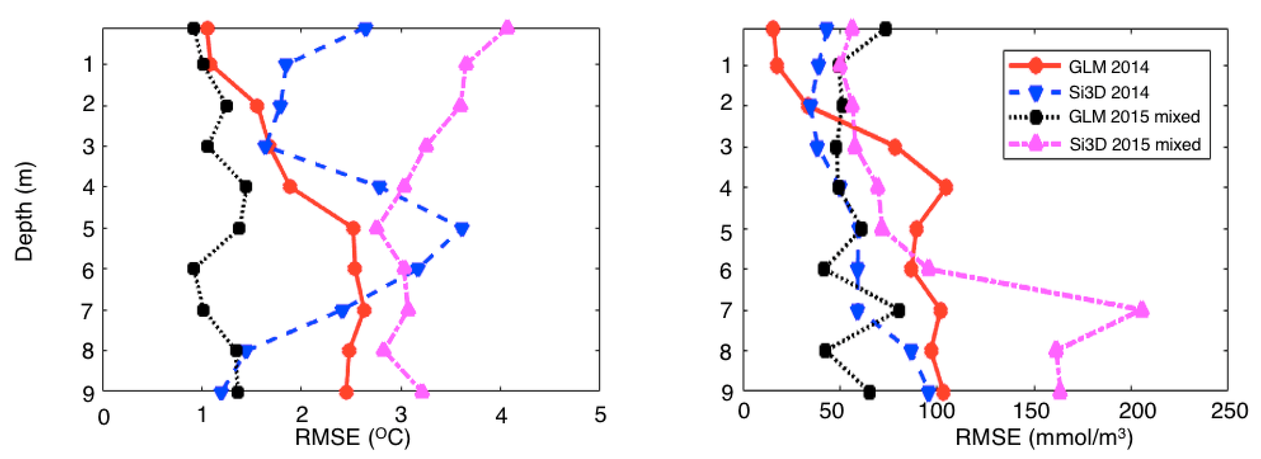
Choosing between 1-D and/or 3-D coupled hydrodynamic and water-quality models for efficient and accurate simulations of natural water bodies is important. In certain circumstances, for example, where the water body is managed to control water quality, it is reasonable to adopt both 1-D and 3-D models for one water body but for different simulation periods. To determine an ideal simulation setup for different engineering scenarios, a community 1-D model and a 3-D hydrodynamic model are coupled with artificial mixing models and the same water-quality model library. The bubble plume model, which is coupled with the community 1-D model for the first time in this study, adequately simulates the bubble plume mixing effect. It is found that the 3-D coupled model adopting the calibrated water-quality parameters from the 1-D model produces satisfactory water-quality results. Based on the comparison between two one-year simulation results using the 1-D and 3-D models for a shallow, eutrophic, managed reservoir, the relative performance of these models is evaluated quantitatively. The 1-D model is recommended when stratification and artificial mixing do not substantially vary during the simulation period, while the 3-D model is recommended to simulate stratification, artificial mixing and spatially sensitive water-quality variables during dynamic periods.

Supplementary Materials

The following are available online at https://www.mdpi.com/2073-4441/13/1/88/s1. The details and results of the numerical tests described in Section 3 are presented in Supplementary Materials.

Author Contributions

The following statements should be used Conceptualization, X.M., C.L., C.C.C., J.C.L.; methodology, X.M., C.L., C.C.C., J.C.L.; software, X.M., C.C.C.; validation, X.M., C.C.C.; formal analysis, X.M., C.C.C.; data curation, X.M, C.C.C.; writing—original draft preparation, X.M.; writing—review and editing, X.M., C.L., C.C.C., J.C.L.; visualization, X.M.; supervision, C.L., C.C.C., J.C.L.; project administration, C.L., C.C.C., J.C.L. All authors have read and agreed to the published version of the manuscript.

Funding

This research was supported by U.S. National Science Foundation grants 1737424 and 1753639.

Institutional Review Board Statement

Not applicable.

Informed Consent Statement

Not applicable.

Data Availability Statement

Software and data used for this study is available through the GitHub repositories. https://github.com/xman2403/1D3D_codes.

Acknowledgments

The authors thank the Reservoir Group at Virginia Tech and FCR Carbon team for field data collection and feedback.

Conflicts of Interest

The authors declare no conflict of interest.

References

  1. Patterson, J.C.; Imberger, J. Simulation of bubble plume destratification systems in reservoirs. Aquat. Sci. 1989, 51, 3–18. [Google Scholar] [CrossRef]
  2. Stepanenko, V.M.; Martynov, A.; Joehnk, K.D.; Subin, Z.M.; Perroud, M.; Fang, X.; Beyrich, F.; Mironov, D.; Goyette, S. A one-dimensional model intercomparison study of thermal regime of a shallow, turbid midlatitude lake. Geosci. Model Dev. 2013, 6, 1337–1352. [Google Scholar] [CrossRef] [Green Version]
  3. Gal, G.; Imberger, J.; Zohary, T.; Antenucci, J.; Anis, A.; Rosenberg, T. Simulating the thermal dynamics of Lake Kinneret. Ecol. Model. 2003, 162, 69–86. [Google Scholar] [CrossRef]
  4. Hamilton, D.P.; Schladow, S. Prediction of water quality in lakes and reservoirs. Part I—Model description. Ecol. Model. 1997, 96, 91–110. [Google Scholar] [CrossRef]
  5. Hu, F.; Bolding, K.; Bruggeman, J.; Jeppesen, E.; Flindt, M.R.; Van Gerven, L.P.A.; Janse, J.H.; Janssen, A.B.G.; Kuiper, J.J.; Mooij, W.M.; et al. FABM-PCLake—Linking aquatic ecology with hydrodynamics. Geosci. Model Dev. 2016, 9, 2271–2278. [Google Scholar] [CrossRef] [Green Version]
  6. Peeters, F.; Traile, D.I.S.; Orke, A.L.; Ivingstone, D.M.L. Earlier onset of the spring phytoplankton bloom in lakes of the temperate zone in a warmer climate. Glob. Chang. Biol. 2007, 13, 1898–1909. [Google Scholar] [CrossRef] [Green Version]
  7. Perroud, M.; Goyette, S.; Martynov, A.; Beniston, M.; Annevillec, O. Simulation of multiannual thermal profiles in deep Lake Geneva: A comparison of one-dimensional lake models. Limnol. Oceanogr. 2009, 54, 1574–1594. [Google Scholar] [CrossRef] [Green Version]
  8. Farrell, K.J.; Ward, N.K.; Krinos, A.I.; Hanson, P.C.; Daneshmand, V.; Figueiredo, R.J.; Carey, C.C. Ecosystem-scale nutrient cycling responses to increasing air temperatures vary with lake trophic state. Ecol. Model. 2020, 430, 109134. [Google Scholar] [CrossRef]
  9. Snortheim, C.A.; Hanson, P.C.; McMahon, K.D.; Read, J.S.; Carey, C.C.; Dugan, H.A. Meteorological drivers of hypo-limnetic anoxia in a eutrophic, north temperate lake. Ecol. Model. 2017, 343, 39–53. [Google Scholar] [CrossRef] [Green Version]
  10. Ward, N.K.; Steele, B.G.; Weathers, K.C.; Cottingham, K.L.; Ewing, H.A.; Hanson, P.C.; Carey, C.C. Differential Responses of Maximum Versus Median Chlorophyll- a to Air Temperature and Nutrient Loads in an Oligotrophic Lake Over 31 Years. Water Resour. Res. 2020, 56. [Google Scholar] [CrossRef]
  11. McKinley, G.; Follows, M.J.; Marshall, J. Mechanisms of air-sea CO2flux variability in the equatorial Pacific and the North Atlantic. Glob. Biogeochem. Cycles 2004, 18, 2011. [Google Scholar] [CrossRef]
  12. Singleton, V.L.; Gantzer, P.; Little, J.C. Linear bubble plume model for hypolimnetic oxygenation: Full-scale validation and sensitivity analysis. Water Resour. Res. 2007, 43. [Google Scholar] [CrossRef] [Green Version]
  13. Six, K.D.; Maier-Reimer, E. Effects of plankton dynamics on seasonal carbon fluxes in an ocean general circulation model. Glob. Biogeochem. Cycles 1996, 10, 559–583. [Google Scholar] [CrossRef]
  14. Cerco, C.F.; Cole, T. Three-Dimensional Eutrophication Model of Chesapeake Bay. J. Environ. Eng. 1993, 119, 1006–1025. [Google Scholar] [CrossRef]
  15. Follows, M.J.; Dutkiewicz, S.; Grant, S.; Chisholm, S.W. Emergent Biogeography of Microbial Communities in a Model Ocean. Science 2007, 315, 1843–1846. [Google Scholar] [CrossRef] [Green Version]
  16. Hoyer, A.B.; Wittmann, M.E.; Chandra, S.; Schladow, S.G.; Rueda, F.J. A 3D individual-based aquatic transport model for the assessment of the potential dispersal of planktonic larvae of an invasive bivalve. J. Environ. Manag. 2014, 145, 330–340. [Google Scholar] [CrossRef]
  17. Acosta, M.; Anguita, M.; Fernández-Baldomero, F.J.; Ramón, C.L.; Schladow, S.G.; Rueda, F.J. Evaluation of a nested-grid implementation for 3D finite-difference semi-implicit hydrodynamic models. Environ. Model. Softw. 2015, 64, 241–262. [Google Scholar] [CrossRef]
  18. Preece, E.P.; Moore, B.C.; Skinner, M.M.; Child, A.; Dent, S. A review of the biological and chemical effects of hypo-limnetic oxygenation. Lake Reserv. Manag. 2019, 35, 229–246. [Google Scholar] [CrossRef]
  19. Singleton, V.L.; Little, J.C. Designing Hypolimnetic Aeration and Oxygenation Systems—A Review. Environ. Sci. Technol. 2006, 40, 7512–7520. [Google Scholar] [CrossRef]
  20. Chen, S.; Little, J.C.; Carey, C.C.; McClure, R.P.; Lofton, M.E.; Lei, C. Three-Dimensional Effects of Artificial Mixing in a Shallow Drinking-Water Reservoir. Water Resour. Res. 2018, 54, 425–441. [Google Scholar] [CrossRef]
  21. Fleischmann, A.S.; Paiva, R.C.D.; Collischonn, W.; Siqueira, V.A.; Paris, A.; Moreira, D.M.; Papa, F.; Bitar, A.A.; Parrens, M.; Aires, F.; et al. Trade-Offs Between 1-D and 2-D Regional River Hydrodynamic Models. Water Resour. Res. 2020, 56, e2019WR026812. [Google Scholar] [CrossRef]
  22. Romero, J.; Antenucci, J.; Imberger, J. One- and three-dimensional biogeochemical simulations of two differing reservoirs. Ecol. Model. 2004, 174, 143–160. [Google Scholar] [CrossRef]
  23. Saloranta, T.M.; Andersen, T. MyLake—A multi-year lake simulation model code suitable for uncertainty and sensitivity analysis simulations. Ecol. Model. 2007, 207, 45–60. [Google Scholar] [CrossRef]
  24. Alobaid, F.; Baraki, N.; Epple, B. Investigation into improving the efficiency and accuracy of CFD/DEM simulations. Particuology 2014, 16, 41–53. [Google Scholar] [CrossRef]
  25. Andersson, A.G.; Hellström, J.G.I.; Andreasson, P.; Lundström, T.S. Effect of Spatial Resolution of Rough Surfaces on Numerically Computed Flow Fields with Application to Hydraulic Engineering. Eng. Appl. Comput. Fluid Mech. 2014, 8, 373–381. [Google Scholar] [CrossRef] [Green Version]
  26. Gerling, A.B.; Munger, Z.W.; Doubek, J.P.; Hamre, K.D.; Gantzer, P.A.; Little, J.C.; Carey, C.C. Whole-Catchment Manipulations of Internal and External Loading Reveal the Sensitivity of a Century-Old Reservoir to Hypoxia. Ecosystems 2016, 19, 555–571. [Google Scholar] [CrossRef]
  27. Munger, Z.W.; Carey, C.C.; Gerling, A.B.; Doubek, J.P.; Hamre, K.D.; McClure, R.P.; Schreiber, M.E. Oxygenation and hydrologic controls on iron and manganese mass budgets in a drinking-water reservoir. Lake Reserv. Manag. 2019, 35, 277–291. [Google Scholar] [CrossRef]
  28. Gerling, A.B.; Browne, R.G.; Gantzer, P.A.; Mobley, M.H.; Little, J.C.; Carey, C.C. First report of the successful operation of a side stream supersaturation hypolimnetic oxygenation system in a eutrophic, shallow reservoir. Water Res. 2014, 67, 129–143. [Google Scholar] [CrossRef]
  29. Chen, S.; Carey, C.C.; Little, J.C.; Lofton, M.E.; McClure, R.P.; Lei, C. Effectiveness of a bubble-plume mixing system for managing phytoplankton in lakes and reservoirs. Ecol. Eng. 2018, 113, 43–51. [Google Scholar] [CrossRef]
  30. Hamre, K.D.; Lofton, M.E.; McClure, R.P.; Munger, Z.W.; Doubek, J.P.; Gerling, A.B.; Schreiber, M.E.; Carey, C.C. In situ fluorometry reveals a persistent, perennial hypolimnetic cyanobacterial bloom in a seasonally anoxic reservoir. Freshw. Sci. 2018, 37, 483–495. [Google Scholar] [CrossRef]
  31. Hanson, P.C.; Weathers, K.C.; Kratz, T.K. Networked lake science: How the Global Lake Ecological Observatory Network (GLEON) works to understand, predict, and communicate lake ecosystem response to global change. Inland Waters 2016, 6, 543–554. [Google Scholar] [CrossRef]
  32. Hipsey, M.R.; Bruce, L.C.; Boon, C.; Busch, B.; Carey, C.C.; Hamilton, D.P.; Hanson, P.C.; Read, J.S.; De Sousa, E.; Weber, M.; et al. A General Lake Model (GLM 3.0) for linking with high-frequency sensor data from the Global Lake Ecological Observatory Network (GLEON). Geosci. Model Dev. 2019, 12, 473–523. [Google Scholar] [CrossRef] [Green Version]
  33. Bruce, L.C.; Frassl, M.A.; Arhonditsis, G.B.; Gal, G.; Hamilton, D.P.; Hanson, P.C.; Hetherington, A.L.; Melack, J.M.; Read, J.S.; Rinke, K.; et al. A multi-lake comparative analysis of the General Lake Model (GLM): Stress-testing across a global observatory network. Environ. Model. Softw. 2018, 102, 274–291. [Google Scholar] [CrossRef] [Green Version]
  34. Read, J.S.; Winslow, L.A.; Hansen, G.J.; Hoek, J.V.D.; Hanson, P.C.; Bruce, L.C.; Markfort, C.D. Simulating 2368 temperate lakes reveals weak coherence in stratification phenology. Ecol. Model. 2014, 291, 142–150. [Google Scholar] [CrossRef] [Green Version]
  35. Hamilton, D.P.; Carey, C.C.; Arvola, L.; Arzberger, P.; Brewer, C.; Cole, J.J.; Gaiser, E.; Hanson, P.C.; Ibelings, B.W.; Jennings, E.; et al. A Global Lake Ecological Observatory Network (GLEON) for synthesising high–frequency sensor data for validation of deterministic ecological models. Inland Waters 2015, 5, 49–56. [Google Scholar] [CrossRef] [Green Version]
  36. Read, J.S.; Hamilton, D.P.; Jones, I.D.; Muraoka, K.; Winslow, L.A.; Kroiss, R.; Wu, C.H.; Gaiser, E. Derivation of lake mixing and stratification indices from high-resolution lake buoy data. Environ. Model. Softw. 2011, 26, 1325–1336. [Google Scholar] [CrossRef]
  37. Chung, E.G.; Schladow, S.G.; Pérez-Losada, J.; Robertson, D.M. A linked hydrodynamic and water quality model for the Salton Sea. Hydrobiologia 2008, 604, 57–75. [Google Scholar] [CrossRef]
  38. Weinstock, J. Vertical turbulence diffusivity for weak or strong stable stratification. J. Geophys. Res. Space Phys. 1981, 86, 9925. [Google Scholar] [CrossRef]
  39. Wüest, A.; Brooks, N.H.; Imboden, D.M. Bubble plume modeling for lake restoration. Water Resour. Res. 1992, 28, 3235–3250. [Google Scholar] [CrossRef]
  40. Haario, H.; Laine, M.; Mira, A.; Saksman, E. DRAM: Efficient adaptive MCMC. Stat. Comput. 2006, 16, 339–354. [Google Scholar] [CrossRef]
  41. Hansen, N.; Müller, S.D.; Koumoutsakos, P. Reducing the Time Complexity of the Derandomized Evolution Strategy with Covariance Matrix Adaptation (CMA-ES). Evol. Comput. 2003, 11, 1–18. [Google Scholar] [CrossRef] [PubMed]
  42. Smith, P.E. A Semi-Implicit, Three-Dimensional Model for Estuarine Circulation. In Open-File Report; U.S. Geological Survey: Reston, VA, USA, 2006. [Google Scholar]
  43. Rueda, F.; Singleton, V.; Stewart, M.; Little, J.; Lawrence, G. Modeling the fate of oxygen artificially injected in the hypolimnion of a lake with multiple basins: Amisk Lake revisited, paper presented at Environmental Hydraulics. In Proceedings of the 6th International Symposium on Environmental Hydraulics, Athens, Greece, 23–25 June 2010; Volume 1, pp. 379–384. [Google Scholar] [CrossRef]
  44. Bruggeman, J.; Bolding, K. A general framework for aquatic biogeochemical models. Environ. Model. Softw. 2014, 61, 249–265. [Google Scholar] [CrossRef] [Green Version]
  45. Courant, R.; Friedrichs, K.; Lewy, H. On the Partial Difference Equations of Mathematical Physics. IBM J. Res. Dev. 1967, 11, 215–234. [Google Scholar] [CrossRef]
  46. McClure, R.P.; Hamre, K.D.; Niederlehner, B.; Munger, Z.W.; Chen, S.; Lofton, M.E.; Schreiber, M.E.; Carey, C.C. Metalimnetic oxygen minima alter the vertical profiles of carbon dioxide and methane in a managed freshwater reservoir. Sci. Total. Environ. 2018, 636, 610–620. [Google Scholar] [CrossRef]
  47. Ladwig, R.; Hanson, P.C.; Dugan, H.A.; Carey, C.C.; Zhang, Y.; Shu, L.; Duffy, C.J.; Cobourn, K.M. Lake thermal structure drives inter-annual variability in summer anoxia dynamics in a eutrophic lake over 37 years. Hydrol. Earth Syst. Sci. Discuss 2020. in review. [Google Scholar] [CrossRef]
  48. Biddanda, B.A.; Weinke, A.D.; Kendall, S.T.; Gereaux, L.C.; Holcomb, T.M.; Snider, M.J.; Dila, D.K.; Long, S.A.; Vandenberg, C.; Knapp, K.; et al. Chronicles of hypoxia: Time-series buoy observations reveal annually recurring seasonal basin-wide hypoxia in Muskegon Lake—A Great Lakes estuary. J. Great Lakes Res. 2018, 44, 219–229. [Google Scholar] [CrossRef]
  49. Kara, E.L.; Hanson, P.C.; Hamilton, D.P.; Hipsey, M.R.; McMahon, K.D.; Read, J.S.; Winslow, L.A.; Dedrick, J.; Rose, K.; Carey, C.C.; et al. Time-scale dependence in numerical simulations: Assessment of physical, chemical, and biological predictions in a stratified lake at temporal scales of hours to months. Environ. Model. Softw. 2012, 35, 104–121. [Google Scholar] [CrossRef]
  50. McDonald, C.P.; Bennington, V.; Urban, N.R.; McKinley, G.A. 1-D test-bed calibration of a 3-D Lake Superior biogeo-chemical model. Ecol. Model. 2012, 225, 115–126. [Google Scholar] [CrossRef]
  51. Toffolon, M.; Serafini, M. Effects of artificial hypolimnetic oxygenation in a shallow lake. Part 2: Numerical modelling. J. Environ. Manag. 2013, 114, 530–539. [Google Scholar] [CrossRef]
Figure 1. Bathymetry contours of Falling Creek Reservoir (FCR) and field data collection sites. The locations of the side stream supersaturation (SSS) system (short white line) and the epilimnion mixing (EM) system (long white line) are also shown.
Water 13 00088 g001
Figure 2. Comparisons of the one-dimensional (1-D, sediment module on, top row) and three dimensional (3-D) model temperature results (middle row) with field data (bottom row). (a) Temperature plot of 2014. (b) Temperature plot of 2015.
Water 13 00088 g002
Figure 3. Comparisons of the 1-D (sediment module on, top row) and 3-D model DO results (middle row) with field data (bottom row). (a) Dissolved oxygen (DO) plot of 2014. (b) DO plot of 2015.
Water 13 00088 g003
Figure 4. Profiles of the RMSEs of the temperature (left) and DO (right) RMSEs of the 1-D and 3-D models for 2014 and the mixed period of 2015.
Water 13 00088 g004
Figure 5. Comparison of the simulated temperature and field data for EM15 at FCR50 (year 2015). The time of the field data collection is indicated by black inverse triangles on the plot of the field data.
Water 13 00088 g005
Figure 6. Comparison of the simulated temperature and field data for EM16–3 at FCR50. The time of the field data collection is indicated by black inverse triangles on the plot of the field data.
Water 13 00088 g006
Figure 7. The field and simulated metalimnion bottom depths during the EM periods of 2015 and 2016.
Water 13 00088 g007
Table 1. Information about the operation of the oxygenation system in the years 2014 and 2015 and the corresponding simulation periods.
YearField Campaign DoYOxygenation SettingsSimulation Period
(DoY)
DoYOxygen Flow Rate (kg/day)Water Flow Rate (L/min)
2014121–310126–15420208121–273
180–21020
230–27325
201590–331125–1521590–331
Table 2. The Si3D-AED2 and GLM-AED2 simulation dates, the EM operation periods and the corresponding flow rates in the years 2015 and 2016.
YearNameSimulation DoYEM Period DoYTimeFlow Rate (L/min)
2015EM15146–15415112:00–15:00708
15312:00–15:00
2016EM16–1 147–15315012:00–18:00708
EM16–2 172–18317812:00–19:00425
19:00–24:00283
1790:00–12:00
EM16–3 202–21320612:00–17:00227
17:00–24:00708
2070:00–12:00
12:00–24:00340
2080:00–12:00
Table 3. The root mean square errors (RMSEs) of the predicted temperatures (in °C) at different depths for 2014 and 2015. The lower RMSEs between the 1-D and 3-D model results for both stratified and mixed conditions are shown in bold.
1-D3-D
2014 *20152014 *2015
StratifiedMixedStratifiedMixed
0.1 m1.051.180.922.643.404.07
3.0 m1.682.391.061.641.643.25
6.0 m2.543.120.923.174.543.03
9.0 m2.451.421.361.203.843.21
Whole lake **1.991.981.172.283.143.25
* FCR is stratified during the 2014 simulation period. ** The whole-lake RMSEs calculate the RMSEs of the variable of interest over 0.1–9 m depths with 1 m resolution.
Table 4. The RMSEs of the predicted DO (in mmol/m3) at different depths for 2014 and 2015. Lower RMSEs between the 1-D and 3-D model results are shown in bold.
1-D3-D
2014 *20152014 *2015
StratifiedMixedStratifiedMixed
0.1 m15.8736.2973.6343.3651.6356.24
3.0 m78.71130.0448.3438.5170.4257.91
6.0 m86.8859.8042.0259.2388.3795.42
9.0 m103.25143.6364.9395.95153.58163.59
Whole lake **72.8496.5056.3156.5989.4498.79
* FCR is stratified during the 2014 simulation period. ** The whole-lake RMSEs calculate the RMSEs of the variable of interest over 0.1–9 m depths with 1 m resolution.
Table 5. The whole-lake normalized mean absolute error (NMAEs) of the predicted temperature and DO for 2014 and 2015. The literature range [8,9,49] is shown in the last row. The relatively lower NMAEs between the 1-D and 3-D model results are shown in bold.
1-D3-DLiterature Range
2014 *20152014 *2015
StratifiedMixedStratifiedMixed
Temperature0.0720.0810.110.0840.120.120.037–0.12
DO0.290.290.180.240.230.320.054–0.33
* FCR is stratified during the Year 2014 simulation period.
Table 6. The RMSEs of the predicted thermocline depths and the metalimnion bottom depths for the entire stratified period of 2014 and 2015 from Si3D and GLM-AED2 simulations. The relatively lower RMSEs between the 1-D and 3-D model results are shown in bold.
Si3D-AED2GLM-AED2
Year2014201520142015
RMSE of the thermocline depth (m)1.71.21.73.0
RMSE of the metalimnion bottom depth (m)2.40.922.32.2
Table 7. RMSEs (in m) of simulated metalimnion bottom depths during the EM periods of 2015 and 2016.
EM15EM16–1EM16–2EM16–3Weighted Average
GLM0.60.610.70.7
Si3D0.50.20.80.30.5
Table 8. The NMAEs of the temperature and DO of the 3-D model at FCR20, FCR30 and FCR45 for the 2014 simulation.
FCR20FCR30FCR45Average
Temperature0.0770.0770.0850.080
DO0.170.160.200.18
Publisher’s Note: MDPI stays neutral with regard to jurisdictional claims in published maps and institutional affiliations.

