Indicative Lake Water Quality Assessment Using Remote Sensing Images-Effect of COVID-19 Lockdown

Abstract

The major lockdown due to the COVID-19 pandemic has affected the socio-economic development of the world. On the other hand, there are also reports of reduced pollution levels. In this study, an indicative analysis is adopted to understand the effect of lockdown on the changes in the water quality parameters for Lake Hussain Sagar using two remote sensing techniques: (i) spectral reflectance (SR) and (ii) chromaticity analysis (Forel-Ule color Index (FUI) and Excitation Purity). The empirical relationships from earlier studies imply that (i) increase in SR values (band B2) indicates a reduction in Chlorophyll-a (Chl-a) and Colored Dissolved Organic Matter (CDOM) concentrations, and (ii) increase in FUI indicates an increase in Total Suspended Solids (TSS). The Landsat 8 OLI satellite images are adopted for comparison between (i) January to May of year 2020: the effect of lockdown on water quality, and (ii) March and April for years 2015 to 2020: historical variations in water quality. The results show notable changes in SR values and FUI due to lockdown compared to before lockdown and after unlock suggesting a significant reduction in lake water pollution. In addition, the historical variations within April suggest that the pollution levels are least in the year 2020.

1. Introduction

The entire globe has witnessed a major socio-economic lockdown due to the spread of the COVID-19 (COronaVIrus Disease-2019) pandemic. This has affected a large proportion of the population worldwide and resulted in significant financial losses due to disruptions in primary activities such as industries and transportation [1]. On the contrary, the critical environmental factors, particularly the quality of air and water bodies across the world, have shown improvements [2,3,4]. These factors significantly impact ecosystems, human health, and overall economic growth, especially for developing countries [5]. Water pollution has been one of India’s crucial challenges over the past few decades due to urbanization, industrialization, poor water quality regulations, and disposal of untreated sewage [6,7,8]. The clean-up and rejuvenation of heavily polluted water bodies pose an enormous monetary liability on the country. Several reports have indicated a betterment of water quality across India over the lockdown period [4,9,10]. The lockdown imposed by the country during the COVID-19 crisis is one of the largest of its kind and halted the entire country’s vital operations. The present study has attempted to explore the effect of COVID-19 lockdown on the urban lake water quality using satellite imagery.

The quality of freshwater bodies depends on diverse anthropogenic, hydrogeological, and environmental factors such as (i) discharge of untreated effluents from industries and residential areas; (ii) proximity of water bodies to agricultural, mining, and waste disposal areas; (ii) possibility of saline water intrusion; (iii) extreme climatic events such as hurricane/storm, drought, and flood; (iv) weather conditions like temperature, rainfall, wind, and evaporation [11,12]; and (v) soil type, aquatic, and terrestrial vegetation. The pollutants reaching water bodies from different sources are subjected to various physical, biological, and chemical attenuation processes and will undergo a considerable reduction in concentration, toxicity, and volume [13,14]. However, the anthropogenic activities substantially influence the self-cleansing process of water bodies [15]. A thorough insight into the effect of anthropogenic activities on water quality is crucial for planning, managing, and implementing the decontamination strategies for the polluted water bodies. As these activities are stalled during the lockdown period, the comparison of water qualities before, during, and after the lockdown period can provide a major understanding of the influence on water quality.

The traditional methods of water quality assessment are carried out either by in situ field sampling or laboratory analysis. Even though these methods provide accurate results, they have certain disadvantages like laborious, slow, restricted to point-scale sampling (limited spatial assessment), and data collection in inaccessible locations [16,17]. Alternatively, aerial and spaceborne Remote Sensing (RS) techniques can be adopted as a viable and cost-effective tool for monitoring the water quality [18,19]. In this technique, the sensors on satellites and other airborne platforms measure the radiation reflected from the water surface at various wavelengths. Each of these wavelengths constitutes a unique spectral signature with the absorption changes indicating the variation in the water quality. Several studies have adopted the spectral reflectance (SR) data obtained from satellite images as a reliable indicator in estimating the changes in water quality [4,20,21,22,23]. Moreover, with the advent of technologies and computational power, these techniques are proving to be vital in decision-making, especially during disasters and pandemics.

On the other hand, the concept of “color” has been used to draw inferences through the human eye for decades. It was envisaged that the “color” of the water is strongly correlated to the water quality. Therefore, one can perceive water as “clean” when there is an absence of blue absorbing and scattering constituents. However, the presence of phytoplankton pigments (if found in predominance), such as Chlorophyll-a (Chl-a), Suspended Particulate Matter (SPM), and Colored Dissolved Organic Matter (CDOM), result in green, yellow, and brown colors of water [24]. The changes in water colors are mainly due to variation in these Optically Active Constituents (OAC). Thus, the color of the water can be used implicitly to indicate water quality. For example, water body with blue or green color is generally recognized as acceptable water quality on the other hand dark brown, grayish brown, or red, indicate water quality anomaly [25].

Chromaticity analysis is widely used for quantitative determination of the color of ocean and inland waters, using the chromaticity parameters, such as Forel–Ule Color Index and Excitation Purity [26,27,28,29,30,31,32,33]. In [34,35], the authors presented the Forel–Ule Color Index (FUI), which can be used as a proxy for natural waters with different optical properties (indicating anomaly in water quality). Oceanographers and limnologists have widely used it since the 19th century. The FUI scale distinguishes the apparent colors of water based on the amount of absorption and scattering of OAC. FUI strongly correlates with turbidity, Secchi Disk Depth (SDD), Chl-a, and CDOM [24,26,28]. FUI is typically observed using a handheld color scale. With the recent advancements of technology, it can also be derived from the remote sensing products (reflectance or water-leaving radiance) and through smartphone apps [28]. FUI scale comprises 21 color standards ranging from blue to green and brown (1: indigo-blue; 21: cola brown) [28]. As water becomes more turbid or muddy due to increasing suspended particulate and dissolved matter, the apparent color of water darkens. This gives higher FUI showing brownish water colors. The light penetration depth given by SDD shows an inverse correlation with both FUI and turbidity [28]. The other chromaticity parameter called Excitation Purity is a qualitative measure of saturation of a color [36].

In this study, it is envisaged that the variations in the water color and SR obtained from the RS data can provide an indicative assessment of the changes in the quality of water bodies. The analysis is similar to the studies carried out in understanding the changes in land use and land cover, vegetation, and soil moisture using RS data [37]. However, it is challenging to quantify the water quality parameters directly from the surface reflectance, unlike land use and land cover classification, wherein the latter has well-established techniques and requires few ground truth values through field studies. Due to the heterogeneous characteristics and limited surface penetration of the electromagnetic spectrum, it is not easy to assess the parameters through remote sensing. However, there are few water quality parameters that are optically active such as Chl-a, CDOM, and TSS which can be monitored using RS. The study presents an indicative comparative analysis using remote sensing data. The changes in the surface reflectance, Forel–Ule color index, and excitation purity will be used to identify the changes in the lake water quality. To understand the effect of COVID-19 pandemic lockdown, the analysis is carried out for (i) before, during, and after lockdown, and (ii) previous years RS data to understand the historical variations. Lake Hussain Sagar, one of the most polluted urban human-made lake water bodies in India, is selected for the analysis.

The paper is organized as follows. Section 2 provides details of the methods and data used for the analysis. This section presents details about indicative analysis using the spectral bands and FUI and their relationship with water quality parameters. Section 3 provides the salient features of the study area. Section 4 presents the results and discussion using the indicative analysis representing the changes in the lake water quality due to lockdown. Finally, in Section 5, the conclusions and limitations of the study are presented.

2. Data and Methods

2.1. Satellite Data

Reflectance is the ratio of total radiation reflected from the surface to the total incoming radiation. In this study, variation in the optical property of the water surface is related to the change in lake water quality. The data sets, data processing methodology, and the statistical approaches to access the differences in the spectral values are as follows. The satellite-based reflectance data are extracted from onboard Landsat 8 sensor Operational Land Imager (OLI). Imagery for the study area was downloaded from Earth Explorer U.S. Geological Survey (USGS) for the required periods [38]. The processed data for the case study can be downloaded at [39]. The salient features of the Landsat 8 spectral bands are presented in

Table 1. Landsat 8 Operational Land Imager (OLI) spectral band details.

Sl. No.	Band	Region in EM Spectrum	Wavelength (nm)	Resolution (m)
1	Band 1	Visible ( Coastal aerosol)	430–450	30
2	Band 2	Visible (Blue)	450–510	30
3	Band 3	Visible (Green)	530–590	30
4	Band 4	Visible (Red)	640–670	30
5	Band 5	Near-Infrared (NIR)	850–880	30
6	Band 6	Short Wave-Infrared 1 (SWIR 1)	1570–1650	30
7	Band 7	Short Wave-Infrared 2 (SWIR 2)	2110–2290	30
8	Band 8	Panchromatic (PAN)	500–680	15
9	Band 9	Cirrus	1360–1380	30

.

OLI captures data with improved radiometric precision over a 12-bit dynamic range, which improves the overall signal to noise ratio. Improved signal to noise performance enables improved characterization of land cover state and condition. In this study, the blue band (Band 2) in the visible range of the electromagnetic (EM) spectrum is used for the surface reflectance based comparative analysis. Note that the other bands can also be associated with the water quality parameters. However, the studies have shown that B2 band reflectance is found to be a dominant factor in water quality assessment [4,40], whereas the visible range bands—band 1 (B1), band 2 (B2), band 3 (B3), and band 4 (B4)—are used in the chromaticity analysis.

2.2. Remote Sensing and Spectral Bands

Remote sensing techniques mainly use three approaches to derive water quality parameters: (i) analytical method, (ii) semi-analytical or semi-empirical method, and (iii) empirical method. In the case of an analytical or model-based approach, the SR is based on the inherent optical properties of the water through radiative transfer modeling [41,42]. The development of a robust model is sophisticated and demands fieldwork, algorithm training, computational time, and knowledge of local Inherent Optical Properties (IOP). The semi-analytical method utilizes the algebraic solution of the reflectance approximation to derive the parameters [43]. Similarly, the semi-empirical method uses absorption features to develop the algorithms correlated to the measured constituents [44]. Empirical methods directly relate the reflectance to the parameter of interest using statistical regression techniques [45,46]. These methods provide robust results for the sites and data sets from which they are derived but lack universality.

Several studies have derived the relationship between the SR and water quality parameters using semi-empirical or empirical methods [47,48,49]. Among various water quality parameters, only a few parameters such as TSS, Chl-a, and CDOM are OAC and thus directly related to the SR [50]. The key reflectance band which is found to be dominant in the literature is in the visible spectrum, specifically the blue band. SR in the blue band is inversely proportional to the concentration of Chl-a and CDOM (

Table 2. List of spectral bands and their relationship with water quality parameters.

Spectral Band	Water Quality Parameters	Inference	References
Blue band	Chl-a	inversely proportional	[47,52,53]
	CDOM	inversely proportional	[40,41,49,54,55,56]

). Thus, the increment in reflectance value of this band will indicate a reduction in the concentration of Chl-a and CDOM. This may be due to the absorption of radiation by these two parameters in wavelengths between 450 and 510 nm [40,51]. The details about the water quality parameters are discussed in the following paragraphs.

2.3. Spectral Analysis of Water Quality Parameters

In general, the water quality assessment involves the analysis of various parameters such as pH, Chlorophyll, Total Dissolves Solids (TDS), hardness, pH, turbidity, Electrical Conductivity (EC), Secchi Disk Depth (SDD), Colored Dissolved Organic Matter (CDOM), Biochemical Oxygen Demand (BOD), Chemical Oxygen Demand (COD), Ammonia Nitrogen (NH3-N), Dissolved Oxygen (DO), Total Phosphorous (TP), Total Nitrogen (TN), alkalinity, chlorides, and other heavy metals. Out of all these water quality parameters, only Chl-a, CDOM, and TSS are Optically Active Constituents (OAC), indicating they interact with electromagnetic radiation and therefore can be inferred using remote sensing techniques [50]. They have unique optical spectral signatures that are detected by the observatory sensors. The rest of the parameters are found to be undetectable through reflectance but can be indirectly evaluated using empirical relations, as they have shown to exhibit a good correlation with OAC. The link between OACs and light signals is the Inherent Optical Properties (IOP) like absorption and backscattering, which are distinct for various constituents. The details about the selected water quality parameters and their spectral characteristics are as follows.

• Chlorophyll pigment in vegetation allows them to create energy by photosynthesis. One of its forms is Chlorophyll-a (Chl-a), which is found in all photosynthesis plants and algae. The presence of Chl-a is used to estimate the amount of suspended algae and the extent of eutrophication in water bodies. Higher water temperatures and longer daylight hours contribute to their growth. The major anthropogenic sources which enhance the Chl-a content in water are untreated sewage, agricultural runoff, and industrial wastes. The extent of damage due to eutrophication can be determined by evaluating Chl-a concentration using the spectral band in visible wavelengths. Chl-a absorbs radiation mainly in the blue (450–520 nm) band [17,20].
• Total suspended solids (TSS) are the inorganic materials comprising of salts and a small quantity of organic matter present in water. An undesirable amount of particulate matter in freshwater bodies increases turbidity, resulting in high nutrient load, and blocks light transmission at the surface, affecting the overall health of aquatic life. Major sources of solids in water bodies are (i) untreated industrial wastes and sewage, (ii) urban land runoff, (iii) agricultural runoff, (iv) bits of decaying vegetation, (v) atmospheric deposition, (vi) wind-driven resuspension, and (vii) phytoplankton (suspended algae). TSS is strongly related to water color or chromaticity, which increases with turbidity [57].
• Colored Dissolved Organic Matter (CDOM) is made up of various macromolecules of carbohydrates, fatty acids, humic substances, and other hydrocarbons, which are an essential source of carbon and energy for heterotrophic organisms living in the water. It indicates the amount of organic carbon resulting from aquatic and terrestrial vegetation (humus) decomposition and soil organic matter of the catchment area. The anthropogenic activities causing an increase in CDOM are untreated domestic sewage, runoff from agricultural land, and animal farms [55]. The presence of high CDOM concentration can also block light from entering the water column, thus reducing the phytoplankton productivity [58,59]. Studies have reported that CDOM absorbs radiation below the 500 nm wavelength [41,46,60]. The optimal concentration is useful in the absorption of UV radiation and hence protects the aquatic biota. However, the high concentration of CDOM is a threat to the functioning of the ecosystem. This compound gives the greenish-brown color to inland water bodies depending on their quantity.

2.4. Satellite Data Processing

The geographically corrected satellite imagery from USGS is processed to convert the Digital Numbers (DN) of the image to the surface reflectance values for the selected bands. This involves three main steps: (i) conversion of DN to spectral radiance using the rescaling factors as proposed in [61], (ii) atmospheric correction for spectral radiance, and (iii) spectral radiance to SR. The last two steps are derived using the improved Dark Object Subtraction (DOS) method [62]. The mathematical form for obtaining the surface reflectance is given as:

2.4.1. Step 1—Conversion of DN to Spectral Radiance

The radiance at satellite sensor, $Lsa{t}_{rad}$$(Watts/\left(m^2\times srad\times \mu m\right))$ of each pixel is calculated using the radiance rescaling factors present in the metadata file for each band.

$$Lsa{t}_{rad}=M_L\times Q_{cal}+A_L$$

(1)

where $M_L$ and $A_L$ are the band-specific multiplicative and additive rescaling factor, respectively, from the metadata file, $Q_{cal}$ = pixel values or DN.

2.4.2. Step 2—Atmospheric Correction

The radiance calculated from Equation (1) has to be corrected for atmospheric scattering by deducting the haze amount (radiance at the sensor that is increased due to the effect of atmospheric haze) from total radiance value.

$$Lhaze1{\%}_{rad}=L{\lambda }_{min}-L\lambda ,1\%$$

(2)

where $L{\lambda }_{min}$ is minimum spectral radiance value at the satellite sensor, $L\lambda$, 1% is the radiance of an object on each band. It is assumed to have a reflectance of 1%.

$$L\lambda ,1\%=0.01\times \frac{Eo\lambda \times cos\theta s}{d^2\times \pi }$$

(3)

where $Eo\lambda$ is the exoatmospheric solar irradiance (also called ESUN$\lambda$), $\theta$ is the sun zenith angle, and $TA{U}_v$ is the atmospheric transmittance along the path from the ground surface to the sensor.

2.4.3. Step 3—Conversion of Radiometrically Corrected Radiance to SR

The SR from the water surface, $\rho \lambda$ is calculated by the following equation,

$$\rho \lambda =\frac{\left(Lsa{t}_{rad}-Lhaze1{\%}_{rad}\right)\pi \times d^2}{Eo\lambda \times cos\theta s\times TA{U}_v}$$

(4)

where d is the distance between earth and sun (in astronomical units), $Lsa{t}_{rad}$ is the spectral radiance at the satellite sensor $(Watts/\left(m^2\times srad\times \mu m\right))$.

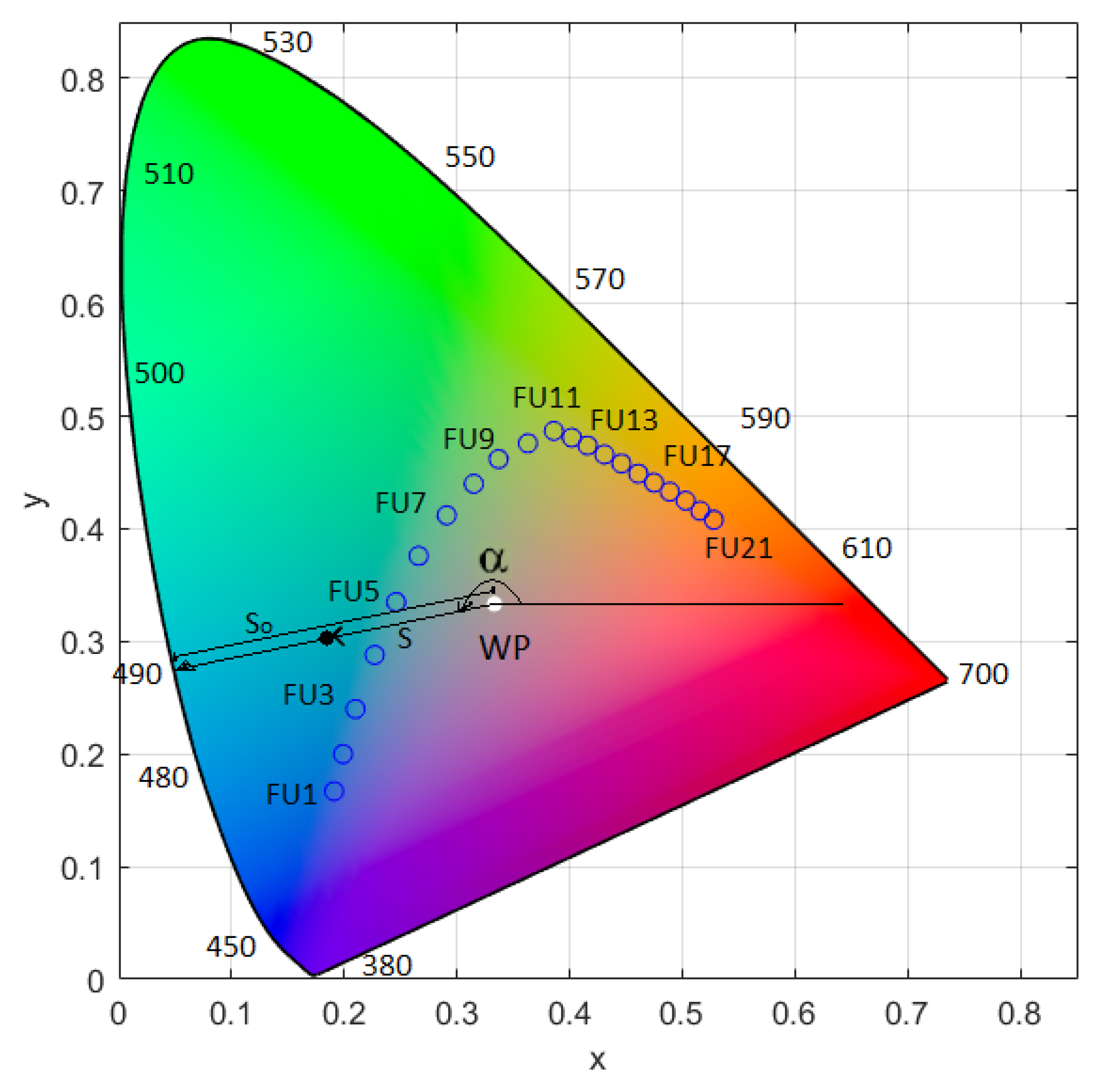
2.5. Forel–Ule Color Index (FUI)

The concept of “color” has been used in several studies for indicative analysis due to its strong correlation with the water quality [26,29]. The International Commission on Illumination (CIE) system provides an approach to describe the “Color” using luminosity, dominant wavelength, and excitation purity (analogous to brightness, hue, and saturation, respectively). The Chromaticity Diagram (Figure 1) helps us plot the hue and saturation values of a particular color [36]. The diagram shows pure spectral colors (truly monochromatic light) on a tilted horseshoe-shaped locus of points. The space enclosed encompasses all possible chromaticity values.

Chromaticity analysis uses three color primaries X, Y, and Z (tristimulus values) to describe the color of an object as perceived by the human eye [24]. The tristimulus values are integrals of the weighted upwelling reflectance spectrum $\rho \left(\lambda \right)$ for 390–740 nm (the region to which the human eye is sensitive). $\overline{x}\left(\lambda \right),\overline{y}\left(\lambda \right)$ and $\overline{z}\left(\lambda \right)$ are weighing functions, which represent the color mixture values based on wavelength dependence of human vision for red, green, and blue light, respectively.

$$X=\underset{390}{\overset{740}{\int }}\rho \left(\lambda \right)\overline{x}\left(\lambda \right)d\left(\lambda \right)$$

(5)

$$Y=\underset{390}{\overset{740}{\int }}\rho \left(\lambda \right)\overline{y}\left(\lambda \right)d\left(\lambda \right)$$

(6)

$$Z=\underset{390}{\overset{740}{\int }}\rho \left(\lambda \right)\overline{z}\left(\lambda \right)d\left(\lambda \right)$$

(7)

The tristimulus values can be reconstructed based on the linear weighted sum of reflectance [27,30] of Landsat 8 OLI bands; Band 1(B1), Band 2(B2), Band 3(B3), and Band 4(B4) as given in Table 1. van der Woerd and Wernand [30] have provided the coefficients for the equations as given below.

$$X=11.053\rho \left(B1\right)+6.950\rho \left(B2\right)+51.135\rho \left(B3\right)+34.457\rho \left(B4\right)$$

(8)

$$Y=1.320\rho \left(B1\right)+21.053\rho \left(B2\right)+66.023\rho \left(B3\right)+18.034\rho \left(B4\right)$$

(9)

$$Z=58.038\rho \left(B1\right)+34.931\rho \left(B2\right)+2.606\rho \left(B3\right)+0.016\rho \left(B4\right)$$

(10)

These individual tristimulus values are normalized to get the chromaticity coordinates x, y, and z, as follows. “White Point (WP)” is the center of the chromaticity diagram at which x = y = z = 1/3 (CIE-E illuminant). Any pair of x, y coordinates can be identified by a hue angle ($\alpha$). It is drawn between a line joining the white point and the x, y coordinate in an anticlockwise direction. The following equation is used to calculate the hue angle.

$$\alpha =arctan(y-(1/3),x-(1/3\left)\right)modulus2\pi$$

(11)

The angles between WP and the FU chromaticity coordinates (${\alpha }_{iT}$) can be used to determine the FUI [63], as shown in the

Table 3. Determination of FUI based Hue angle for i = 1 to 21 as shown in Figure 1.

i	${\mathit{\alpha }}_{\mathit{iT}}$	If $\mathit{\alpha }$ > ${\mathit{\alpha }}_{\mathit{iT}}$, Then FUI =		i	${\mathit{\alpha }}_{\mathit{iT}}$	If $\mathit{\alpha }$ > ${\mathit{\alpha }}_{\mathit{iT}}$, Then FUI =
1	227.168	1		12	62.186	12
2	220.977	2		13	56.435	13
3	209.994	3		14	50.665	14
4	190.779	4		15	45.129	15
5	163.084	5		16	39.769	16
6	132.999	6		17	34.906	17
7	109.054	7		18	30.439	18
8	94.037	8		19	26.337	19
9	83.346	9		20	22.741	20
10	74.572	10		21		21
11	67.572	11

.

The correction ($▵\alpha$) is applied to hue angle as described by van der Woerd and Wernand [27], van der Woerd and Wernand [30]. The coefficients of the following equations for Landsat 8 OLI are also provided in [30].

$$▵\alpha =-52.16a^5+373.81a^4-981.83a^3+1134.19a^2-533.61a76.72$$

(12)

where, a = $\alpha$ / 100.

Excitation Purity (S*)

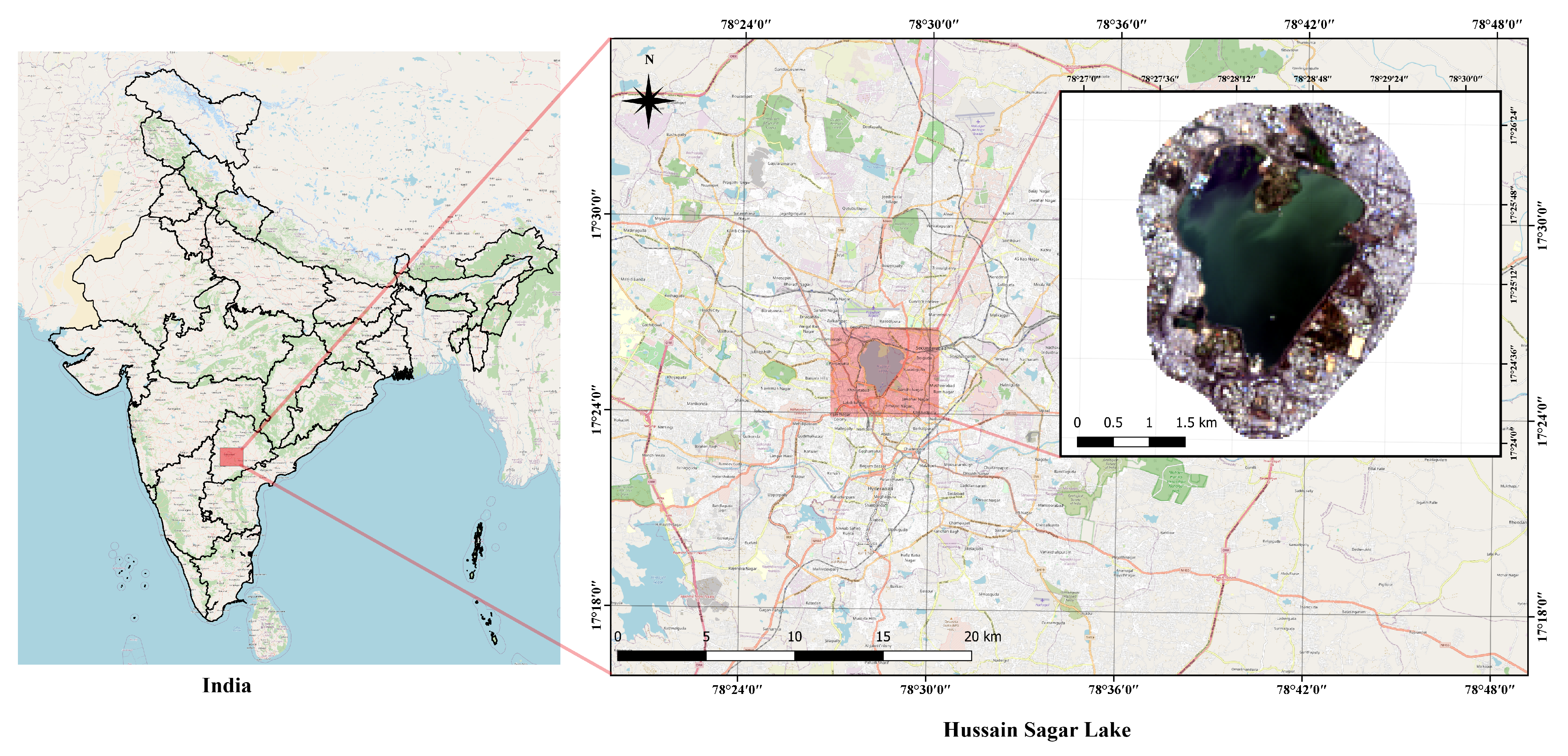
Excitation purity (S*) is a qualitative measure of saturation of a particular color, i.e., how similar the color is to its dominant wavelength. It is the ratio of the distance between WP and x, y coordinates (S) to the distance between WP and spectral locus of the dominant wavelength, $\left(S_o\right)$ [36]. The corrected hue angle ($\alpha +▵\alpha$) is used to determine the dominant wavelength by constructing a line between the x, y coordinates, and WP, and then extrapolating the line until it intersects the locus of the chromaticity diagram. Similar to hue angle correction, a correction ($▵S$ ) is applied to S as suggested by Lehman et al. [24].

$$▵S=-0.0099a^5+0.1199a^4-0.4594a^3+0.7515a^2-0.5095a+0.1222$$

(13)

Thus, excitation purity is given as

$$S^{*}=\frac{S+▵S}{S_o}$$

(14)

3. Study Area

During the lockdown, the most affected activities which directly influence the pollution characteristics of the water bodies are (i) commercial/small-scale businesses, (ii) transportation, (iii) industries, (iv) educational institutions, and (v) tourism [1,4,64]. In this study, Lake Hussain Sagar (HS), one of the most polluted urban water bodies in India, is selected for the analysis. The Lake HS is located at the heart of the city (as shown in Figure 2), and the pollution is mainly due to the domestic sewage (generated from commercial locations, educational institutions, and industries), industrial effluents, and storm sewage.

Lake HS (latitude 15 N and longitude 81 E) is the largest human-made lake in Asia built in the year 1562 A.D. It was constructed to meet the drinking water and irrigation water demands of the twin cities Hyderabad and Secunderabad during the years 1894–1930. The lake is also known as Tank Bund, as initially it is constructed by forming a bund. The lake was once famous for the aquatic life and particularly for the delicious Murrel fish and a stopover point for the migrating birds, including flamingos. It is also a popular spot for sailing. The 16 m high Buddha statue, also known as India’s “Statue of Liberty”, has been a huge attraction for many tourists. This has given rise to boating in the lake. The full tank level of the lake is about 513 m above the mean sea level. The total catchment area of the lake is 240 sq.km, where the present water spread area at full tank level is 4.73 sq.km. The average depth at full capacity is 5.02 m. The shoreline length is about 14 km. The lake is fed by four incoming major drains ($nalas$): Kukatpally $nala$, Picket $nala$, Banjara $nala$, and Balkapur $nala$. Along with untreated domestic sewage, Kukatpally $nala$ also drains industrial effluents into the lake [65]. The increased pollution of the lake has led to a huge reduction in aquatic life. One of the major goals of the local municipalities is to restore the lake as a freshwater source for the city and recreation purposes.

4. Results and Discussion

The level-1 Landsat 8 satellite images for bands B1, B2, B3, B4, and B5 are downloaded from the USGS for the pre- and post-conditions of the first COVID-19 lockdown in India. The available satellite data for the case study was coincidentally before (25 March), during (14 April), and after (2 May) the first lockdown period. The satellite imagery for indicative analysis is collected for (i) January to May 2020 to study the lockdown effect, and (ii) March and April for years 2015 to 2020 to study the historical variations. In the year 2020, no cloud-free images were available for the month of February. The details of all the selected data (97–98% cloud free images) are provided in

Table 4. Details of the Landsat 8 OLI images of lake Hussain Sagar used in this study covering Path 144—Row 48. Cloud-free satellite images are only selected in the analysis. No could-free satellite images were found in February 2020. For historical variations, only the months March and April during years 2015 to 2020 are considered.

Sl. No.	Year	Date of Image Captured	Image ID	Remarks
1	2020	2 May	LC08_L1TP_144048_20200502_20200509_01_T1	Initial unlock
2		16 April	LC08_L1TP_144048_20200416_20200423_01_T1	During lockdown
3		15 March	LC08_L1TP_144048_20200315_20200325_01_T1	Before lockdown
4		27 January	LC08_L1TP_144048_20200127_20200210_01_T1	-
5	2019	14 April	LC08_L1TP_144048_20190414_20190422_01_T1	-
6		29 March	LC08_L1TP_144048_20190329_20190404_01_T1	-
7	2018	27 April	LC08_L1TP_144048_20180427_20180502_01_T1	-
8		10 March	LC08_L1TP_144048_20180310_20180320_01_T1	-
9	2017	24 April	LC08_L1TP_144048_20170424_20170502_01_T1	-
10		23 March	LC08_L1TP_144048_20170323_20170329_01_T1	-
11	2016	21 April	LC08_L1TP_144048_20160421_20170326_01_T1	-
12		20 March	LC08_L1TP_144048_20160320_20170327_01_T1	-
13	2015	19 April	LC08_L1TP_144048_20150419_20170409_01_T1	-
14		18 March	LC08_L1TP_144048_20150318_20170412_01_T1	-

. In this study, the water quality of the lake HS is studied using two indicative remote sensing based analysis: (i) spatio-temporal variation of Band B2 surface reflectance and (ii) chromaticity analysis such as FUI and Excitation Purity.

The variations in the SR is restricted to B2 band as most of the studies indicate that this band is highly correlated to water quality, mainly Chl-a and CDOM [17,20,41,46]. The atmospherically corrected B2 reflectance band image for the lake HS before and during lockdown is shown in Figure 3. Through visual inspection of Figure 3, it is evident that the reflectance (false color) of the lake surface is different for the selected periods indicating changes in the water quality. In Figure 3, it is observed that the SR of the lake during lockdown (April 2020) shows higher reflectance (brighter) when compared to March 2020.

In order to understand the differences in the variations of the reflectance before, during, and after lockdown, further analysis of the data is carried out by mapping the Empirical Cumulative Distribution Functions (ECDF) and quantiles of surface reflectance values over the lake as shown in Figure 4 and Figure 5. The ECDF and Q-Q plots provide statistical insights on the spatial variations of the SR values for a given water body and help to understand the spatio-temporal characteristics of the water quality. Quantile–Quantile (Q–Q) is a graphical technique to compare two datasets’ statistical characteristics without fitting any distributions or finding the unknown parameters. A reference line is a 45line and the deviation of plots from the reference line help to draw inferences about how the two samples differ from each other. The Q–Q plot lies on the reference line if both the datasets have same statistical parameters. The plot lies above the reference line if the latter dataset has a higher mean or location parameter than the former. Slope of the plot increases more than the reference line when the standard deviation of latter dataset is more than former. The earlier studies (Section 2) indicate that increment in B2 band reflectance values shows a decrease in Chl-a and CDOM concentrations.

The FUI has been widely used in indicative analysis to understand variations in the ocean and inland water quality [26,27,28,29,30,31,32,33]. The water colors can be assigned with FUI ranging from 1 (indigo-blue) to 21 (cola-brown). The higher FUI show brownish water color indicating turbidity due to suspended particulate and dissolved matter, thus reducing the light penetration depth value (SDD) [28]. On the other hand, lower FUI (blue water color) indicates clear water [29]. Figure 4c and Figure 6a show the FUI comparison in the year 2020 (Jan–May) and previous years (2015–2019) for the months of March and April. In addition, the study uses excitation purity to analyze the saturation of a particular color which is useful in analyzing the spatial variation of the color in the water body. The purity percentage is compared between March and April for the years 2015–2020 as shown in Figure 6b.

4.1. Before, during and after Lockdown

Indicative analysis of B2 band SR and FUI for months January, March, April, and May in the year 2020 is illustrated in Figure 4. The major observations are listed below.

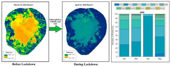
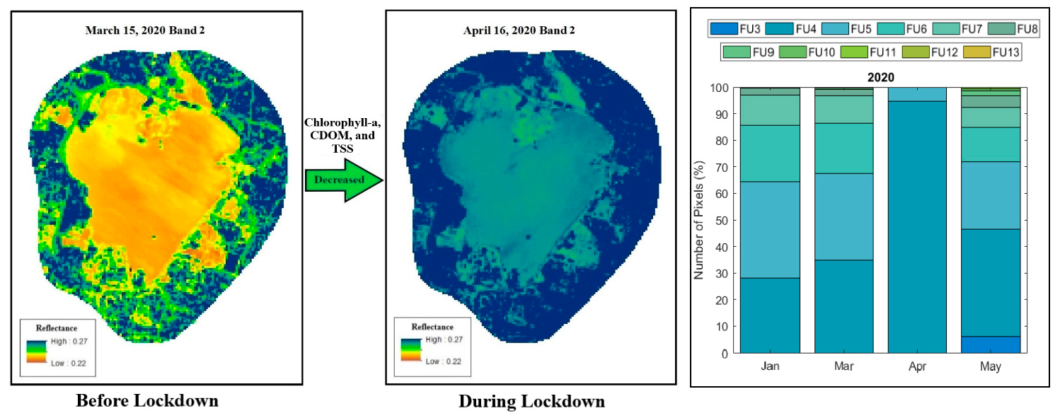
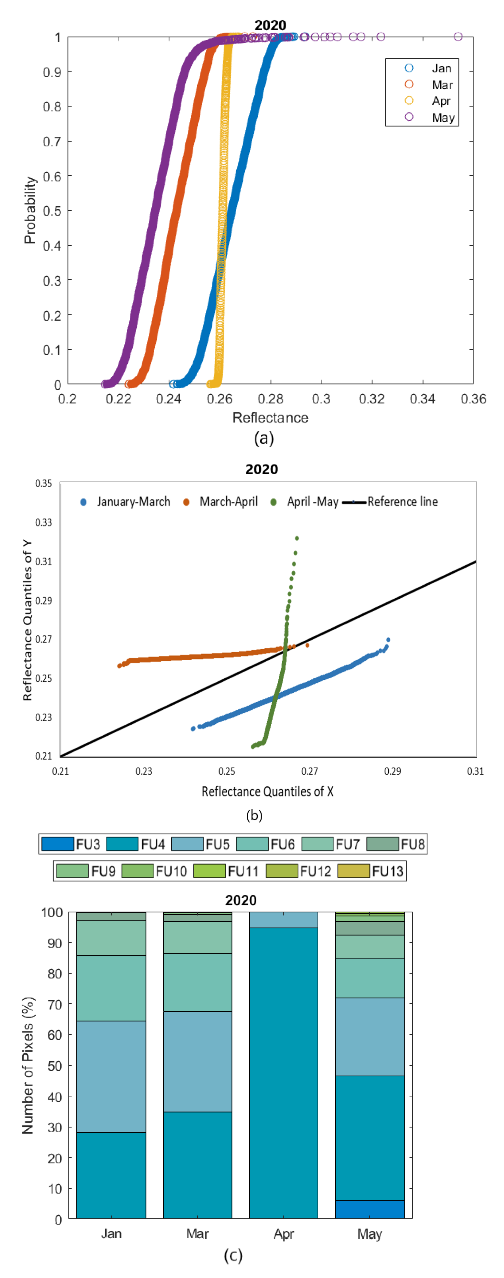
• ECDF (Figure 4a): The SR for April 2020 has increased when compared to January, March, and May 2020. This indicates that there is an improvement in the water quality in April (i.e., decreased Chl-a and CDOM (Section 2)). The SR values of before lockdown and after unlock are similar, indicating an increase in pollution after unlock. SR values for the month of April have the smallest range, unlike other months, which implies that the SR values are uniformly distributed over the lake.
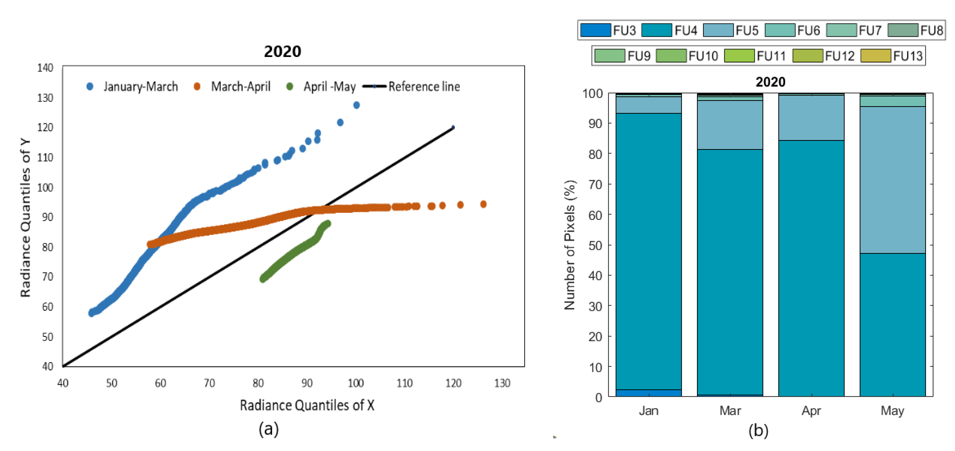
• Q–Q analysis (Figure 4b): It is evident from the figure that there are considerable changes in the SR values for March–April when compared to the changes in other months. Further, the SR values clearly lie above the reference line because the reflectance has increased in April compared to March. It is to be noted that after unlock, the Q–Q plot for April-May indicates there is a decrease in SR values, i.e., a decrease in lake water quality. In addition, the January–March and April–May lines lie below the 45reference line, which shows that the reflectance has decreased in March and May due to an increase in Chl-a and CDOM levels in the before lockdown and after unlock months. The March–April line has a mild slope indicating that the standard deviation in April is less than that in March and May.
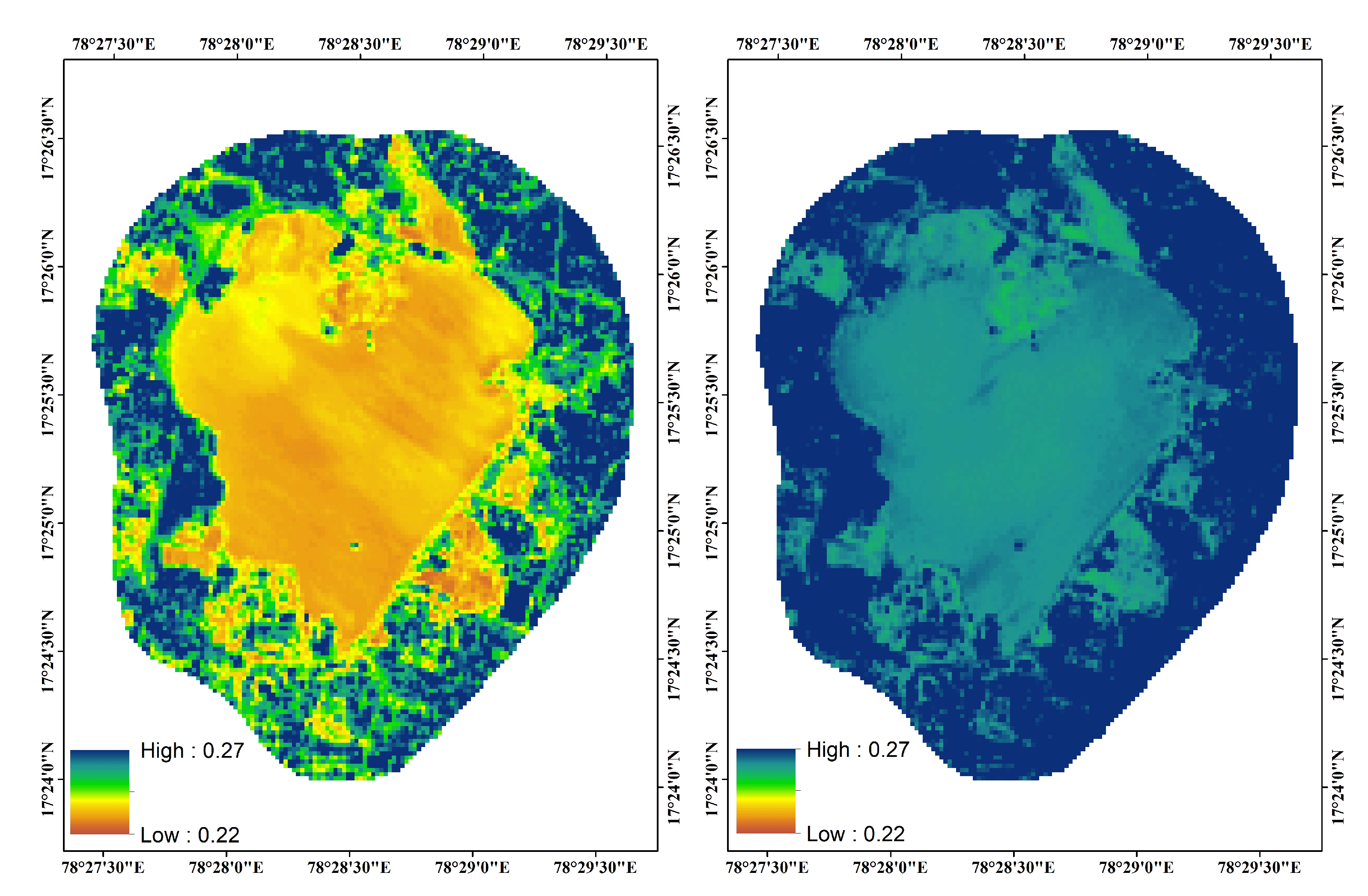
• FUI (Figure 4c): The maximum number of pixels (95%) have low FUI in month April 2020, when compared to the before lockdown and after unlock months, indicating there is a decrease in turbidity of the lake. This might be due to the decrease in TSS concentration [28] and an increase in SDD [31]. In case of unlock phase (May, 2020), the FUI index (50% of pixels) increases similar to the before lockdown phase (March, 2020). It is worth noting that in the month May due to the initial unlock effect, it shows 50% of the pixels with higher FUI (greater than 4), which is very similar to the pre-lockdown conditions. Further, in both before lockdown and unlock conditions the spatial FUI of the lake is similar. On the other hand, April 2020 shows the maximum number of pixels (95%) having a uniform water color with the least FUI (FU4).

4.2. Historical Variations (2015–2020)

The monthly variability of SR in the months March and April for years 2015 to 2020 are analyzed using ECDF, Q-Q, FUI and Excitation Purity plots (Figure 5 and Figure 6). Our observations are listed below.

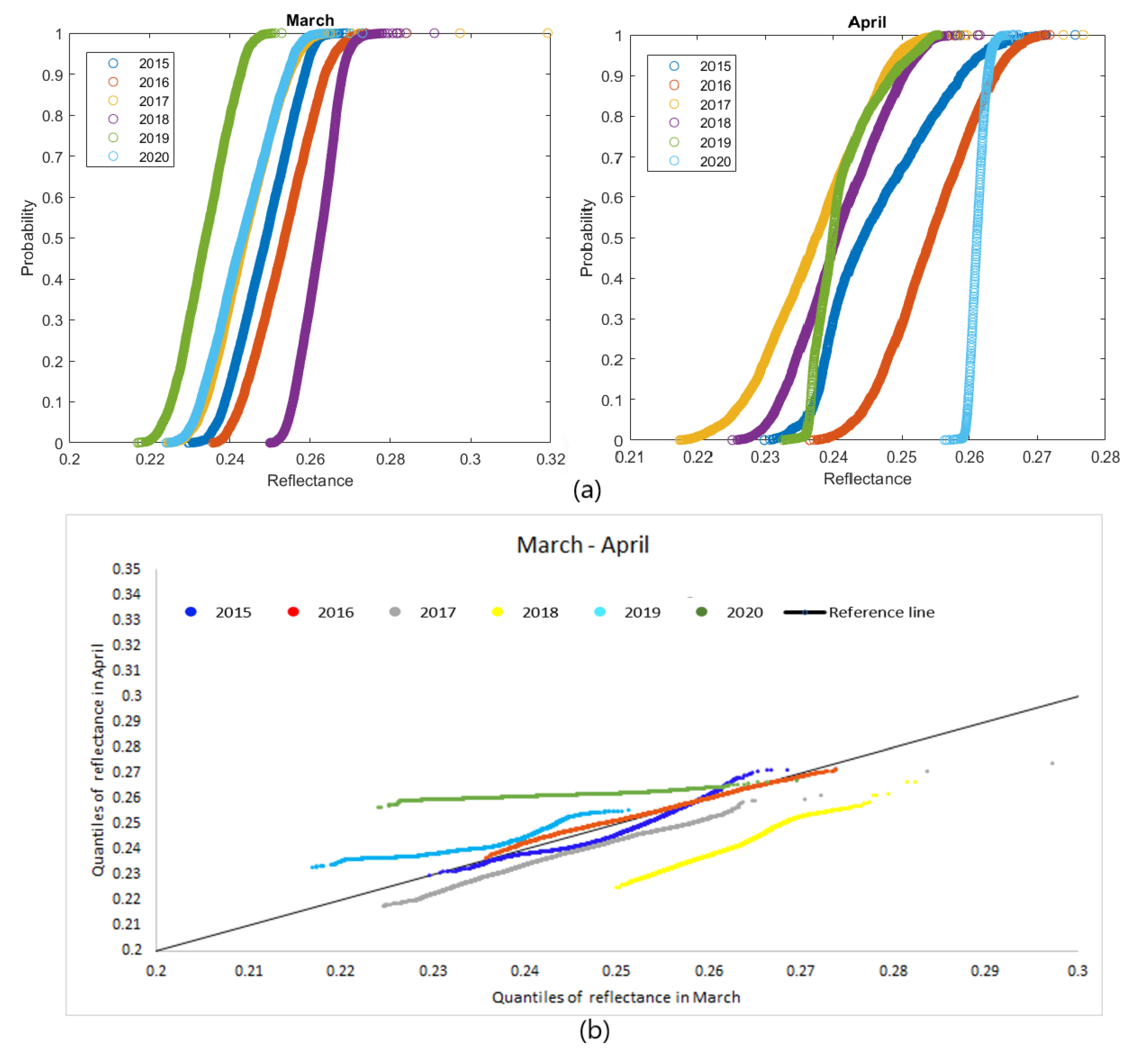
• ECDF (Figure 5a): Except for April 2020, both March and April months show similar behavior in SR values for all the given years. For April 2020, B2 has a considerable increase in the SR values in comparison to the previous years. Furthermore, the range of B2 SR values is consistent for all pixels of the lake in April 2020 as discussed earlier.
• Q–Q plot (Figure 5b): The March–April Q–Q plot clearly shows that the inter-month (March–April) for the year 2020 lies above the reference line when compared to the previous years. This clearly implies an improvement in water quality in month April 2020 due to the lockdown. In the previous years, the mean reflectance is nearly the same (line parallel to reference line) or lower than March (line below reference line).
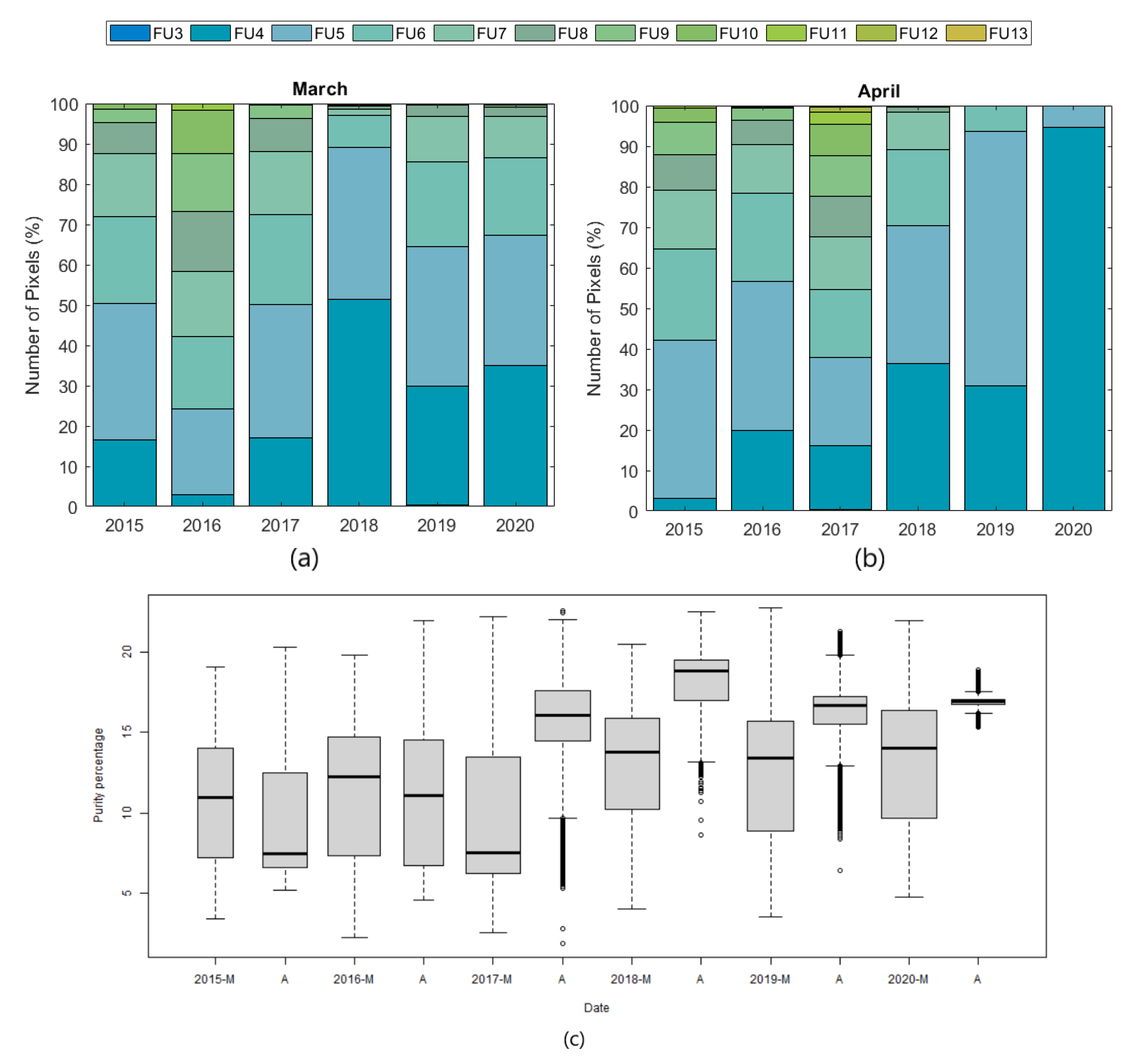
• FUI (Figure 6a): It is expected to have variations in the water colors throughout the lake HS due to its multiple effluent inlets, indicating nonuniform water color (FUI) throughout the lake area. This can be seen through the FUI variations in March and April months for all the given years. However, April 2020 shows a maximum number of pixels with a uniform color with the least FUI (FU4) compared to all the given years. This implies the improvement and uniformity in the watercolor over the maximum lake area. As no industrial effluents were discharged in the lake during the lockdown, the lake water quality has improved and the water color is uniform over the lake area.
• Excitation Purity (Figure 6b): This refers to qualitative measure of water color saturation. The box plot for purity percentage representing the spatial variations in water color saturation over the lake area. The figure indicates that in month April 2020, the purity percentage is found to be consistent throughout the lake area when compared to the other months and previous years. The effect of lockdown on excitation purity is clearly visible in April 2020 box plot.

It is evident from the results that the trend in SR has considerably changed in April 2020 due to the lockdown when compared to the previous years (2015–2019). The significant increase in SR during April 2020 could imply a reduction in Chl-a and CDOM concentrations in the lake water. Similarly, FUI in April 2020 is found to be uniform and minimum FUI over the lake area, indicating decrease in turbidity and TSS concentration due to low industrial effluent influx in the lake.

4.3. Satellite Imagery: Effect of Atmospheric Correction

Satellite image quality is affected by the molecules (such as gases and water vapor) and aerosols present in the atmosphere, which cause scattering and absorption of sunlight. This increases the top of atmosphere reflectance (radiance) due to the additional path or scattering (as shown in Equation (1) which does not account for the influence of atmospheric haze). Therefore, the atmospheric correction is carried out to remove the effect of haze Equation (2). It is evident from Q–Q plots and FUI (Figure 4 and Figure 7) that the radiance is unable to capture the near field conditions when compared to the surface reflectance. Especially in the FUI analysis, radiance shows no variations in the FU color when compared to that of surface reflectance. This implies that the radiance will not be effective in the indicative analysis for detecting the changes in water quality. Thus the atmospheric correction plays a significant role in deriving the surface reflectance from satellite imagery [66].

5. Summary and Conclusions

This study compares the effect of COVID-19 lockdown on the changes in the water quality parameters for lake Hussain Sagar using the remote sensing techniques. It is envisaged that the changes in the SR values and FUI (water color) over the lockdown period indicate changes in the water quality of the lake. In this study, an indicative analysis using (i) spatio-temporal variation of Band B2 SR and (ii) chromaticity analysis, such as FUI and Excitation Purity, is carried out. It is evident from the results that due to the lockdown the lake had a significant effect on the pollution characteristics when compared to the previous years (2015–2019), suggesting a considerable reduction in the concentrations of Chl-a, CDOM, and TSS. Water quality cannot be uniform throughout the water body [67]. However, this study shows that during the lockdown, the concentration levels in the lake are found to be more uniformly distributed when compared to before lockdown and after unlock (2020) or previous years (2015–2019). This suggests that the lake pollutant concentrations are uniformly distributed on the lake surface due to low effluent influx during the lockdown. Reduction in pollutant levels was due to restrictive measures to limit the anthropogenic activities and closure of several large and small-scale industries in the city of Hyderabad.

Major Limitations and Extension

• The comparison analysis is based on the SR (qualitative relationships with OAC) and FUI. The field observations will be required to quantify the actual concentration levels and changes in the lake water quality. However, in the absence of these values, it is envisaged that the indicative analysis of remote sensing images are useful for stakeholders and decision-makers.
• The study is restricted to only three water quality parameters: Optically Active Constituents (OAC) Chl-a, CDOM, and TSS. However, there are other important parameters such as pH, DO, BOD, and COD which need to be evaluated for effective water quality management. There are limited studies that are successful in relating the SR values to non-OAC parameters and hence unable to provide any assessment on these parameters. This indicates that for effective management of water quality of large lakes, both remote sensing and continuous field-based monitoring is essential. This can help generate a large dataset for developing spatio-temporal empirical relationship for the water quality parameters.
• In this study, Landsat 8–30 m resolution data are used. The high-resolution data can provide greater insights into the variations of the lake SR and FUI values. Moreover, the higher resolution images can help in investigating the water quality variations of smaller water bodies, including rivers.
• The study is restricted to the B2 (blue) band and its empirical relationship with pollutants Chl-a, CDOM, and TSS. However, there are other important bands and band ratios such as B3/B2, B5/B4, B2/B4, and NDVI, which can be used in developing empirical relations [48,68]. Further, it is observed that there is a limited consistency among these ratios and water quality parameters when compared to B2 band. The study is in progress to understand these ratios over various scenarios, as discussed in point 5.
• The study is in progress to develop a similar analysis for several large water bodies across the globe to understand the variations of SR and FUI over different scenarios such as urban vs. non-urban, developed vs. developing countries, various climate scenarios (humid vs. arid vs. cold), and coastal vs. inland lakes. In addition, the monitoring of these lakes will be continued during the subsequent lockdown periods in India. Efforts are being made to collect the ground truth values for these lakes.

References

1. Arora, S.; Bhaukhandi, K.; Mishra, P. Coronavirus lockdown helped the environment to bounce back. Sci. Total. Environ. 2020, 742. [Google Scholar] [CrossRef] [PubMed]
2. Braga, F.; Scarpa, G.M.; Brando, V.E.; Manfè, G.; Zaggia, L. COVID-19 lockdown measures reveal human impact on water transparency in the Venice Lagoon. Sci. Total. Environ. 2020, 736, 139612. [Google Scholar] [CrossRef] [PubMed]
3. Hallema, D.; Robinne, F.; McNulty, S. Pandemic spotlight on urban water quality. Ecol. Process 2020, 9. [Google Scholar] [CrossRef] [PubMed]
4. Yunus, A.P.; Masago, Y.; Hijioka, Y. COVID-19 and surface water quality: Improved lake water quality during the lockdown. Sci. Total. Environ. 2020, 731, 139012. [Google Scholar] [CrossRef] [PubMed]
5. Chakraborty, I.; Maity, P. COVID-19 outbreak: Migration, effects on society, global environment and prevention. Sci. Total. Environ. 2020, 728, 138882. [Google Scholar] [CrossRef]
6. Amrutha, K.; Warrier, A. The first report on the source-to-sink characterization of microplastic pollution from a riverine environment in tropical India. Sci. Total. Environ. 2020, 739, 140377. [Google Scholar] [CrossRef]
7. Bhardwaj, S.; Soni, R.; Gupta, S.; Shukla, D.P. Mercury, arsenic, lead and cadmium in waters of the Singrauli coal mining and power plants industrial zone, Central East India. Environ. Monit. Assess. 2020, 192, 251. [Google Scholar] [CrossRef] [PubMed]
8. Duttagupta, S.; Mukherjee, A.; Bhattacharya, A.; Bhattacharya, J. Wide exposure of persistent organic pollutants (PoPs) in natural waters and sediments of the densely populated Western Bengal basin, India. Sci. Total. Environ. 2020, 717, 137187. [Google Scholar] [CrossRef] [PubMed]
9. Mishra, D.R.; Kumar, A.; Muduli, P.R.; Equeenuddin, S.M.; Rastogi, G.; Acharyya, T.; Swain, D. Decline in Phytoplankton Biomass along Indian Coastal Waters due to COVID-19 Lockdown. Remote. Sens. 2020, 12, 2584. [Google Scholar] [CrossRef]
10. Aman, M.A.; Salman, M.S.; Yunus, A.P. Some respite for India’s dirtiest river? Examining the Yamuna’s water quality at Delhi during the COVID-19 lockdown period. Sci. Total. Environ. 2020, 20, 100382. [Google Scholar] [CrossRef]
11. Chawla, I.; Karthikeyan, L.; Mishra, A.K. A Review of Remote Sensing Applications for Water Security: Quantity, Quality, and Extremes. J. Hydrol. 2020, 585, 124826. [Google Scholar] [CrossRef]
12. Mokarram, M.; Saber, A.; Sheykh, V. Effects of heavy metal contamination on river water quality due to the release of industrial effluents. J. Clean. Prod. 2020. [Google Scholar] [CrossRef]
13. Glaser, C.; Zarfl, C.; Werneburg, M.; Böckmann, M.; Zwiener, C.; Schwientek, M. Temporal and spatial variable in-stream attenuation of selected pharmaceuticals. Sci. Total. Environ. 2020, 741, 139514. [Google Scholar] [CrossRef] [PubMed]
14. Ollivier, P.; Engevin, J.; Bristeau, S.; Mouvet, C. Laboratory study on the mobility of chlordecone and seven of its transformation products formed by chemical reduction in nitisol lysimeters of a banana plantation in Martinique (French Caribbean). Sci. Total. Environ. 2020, 743, 140757. [Google Scholar] [CrossRef]
15. Zereg, S.; Boudoukha, A.; Benaabidate, L. Impacts of natural conditions and anthropogenic activities on groundwater quality in Tebessa plain, Algeria. Sustain. Environ. Res. 2018, 28(6), 340–349. [Google Scholar] [CrossRef]
16. Korostynska, O.; Mason, A.; Al-Shamma’a, A. Monitoring Pollutants in Wastewater: Traditional Lab Based versus Modern Real-Time Approaches. In Smart Sensors for Real-Time Water Quality Monitoring, Smart Sensors, Measurement and Instrumentation; Springer: Berlin/Heidelberg, Germany, 2013; Volume 4. [Google Scholar]
17. Gholizadeh, M.H.; Melesse, A.M.; Reddi, L. A Comprehensive Review on Water Quality Parameters Estimation Using Remote Sensing Techniques. Sensors 2016, 16, 1298. [Google Scholar] [CrossRef] [Green Version]
18. Franch-Pardo, I.; Napoletano, B.M.; Rosete-Verges, F.; Billa, L. Spatial analysis and GIS in the study of COVID-19. A review. Sci. Total. Environ. 2020, 739, 140033. [Google Scholar] [CrossRef]
19. Muhammad, S.; Long, X.; Salman, M. COVID-19 pandemic and environmental pollution: A blessing in disguise? Sci. Total. Environ. 2020, 728, 138820. [Google Scholar] [CrossRef]
20. Song, K.; Wang, Z.; Blackwell, J.; Zhang, B.; Li, F.; Zhang, Y.; Jianga, G. Water quality monitoring using Landsat Themate Mapper data with empirical algorithms in Chagan Lake, China. J. Appl. Remote. Sens. 2011, 5, 53506. [Google Scholar] [CrossRef]
21. Hafeez, S.; Wong, M.S.; Abbas, S.; Kwok, C.Y.T.; Nichol, J.; Lee, K.H.; Tang, D.; Pun, L. Detection and Monitoring of Marine Pollution Using Remote Sensing Technologies. In Monitoring of Marine Pollution, Houma Bachari Fouzia; InTech Open: Rijeka, Croatia, 2018. [Google Scholar]
22. Sheffield, Z.; Wood, E.; Pan, M.; Beck, H.; Coccia, G.; Serrat-Capdevila, A.; Verbist, K. Satellite Remote Sensing for Water Resources Management: Potential for Supporting Sustainable Development in Data-Poor Regions. Water Resour. Res. 2018, 54, 9724–9758. [Google Scholar] [CrossRef] [Green Version]
23. Niroumand-Jadidi, M.; Bovolo, F.; Bruzzone, L. Novel Spectra-Derived Features for Empirical Retrieval of Water Quality Parameters: Demonstrations for OLI, MSI, and OLCI Sensors. IEEE Trans. Geosci. Remote. Sens. 2019, 57, 10285–10300. [Google Scholar] [CrossRef]
24. Lehmann, M.K.; Nguyen, U.; Allan, M.; van der Woerd, H.J. Colour Classification of 1486 Lakes across a Wide Range of Optical Water Types. Remote. Sens. 2018, 10, 1273. [Google Scholar] [CrossRef] [Green Version]
25. Zhao, Y.; Shen, Q.; Wang, Q.; Yang, F.; Wang, S.; Li, J.; Zhang, F.; Yao, Y. Recognition of Water Colour Anomaly by Using Hue Angle and Sentinel 2 Image. Remote. Sens. 2020, 12, 716. [Google Scholar] [CrossRef] [Green Version]
26. Wernand, M.R.; van der Woerd, H.J.; Gieskes, W.W.C. Trends in Ocean Colour and Chlorophyll Concentration from 1889 to 2000, Worldwide. PLoS ONE 2013, 8, e63766. [Google Scholar] [CrossRef]
27. Van der Woerd, H.J.; Wernand, M.R. True Colour Classification of Natural Waters with Medium-Spectral Resolution Satellites: SeaWiFS, MODIS, MERIS and OLCI. Sensors 2015, 15, 25663–25680. [Google Scholar] [CrossRef] [Green Version]
28. Garaba, S.P.; Friedrichs, A.; Voß, D.; Zielinski, O. Classifying Natural Waters with the Forel-Ule Colour Index System: Results, Applications, Correlations and Crowdsourcing. Int. J. Environ. Res. Public Health 2015, 12, 16096–16109. [Google Scholar] [CrossRef] [Green Version]
29. Li, J.; Wang, S.; Wu, Y.; Zhang, B.; Chen, X.; Zhang, F.; Shen, Q.; Peng, D.; Tian, L. MODIS observations of water color of the largest 10 lakes in China between 2000 and 2012. Int. J. Digit. Earth 2016, 9, 788–805. [Google Scholar] [CrossRef]
30. van der Woerd, H.J.; Wernand, M.R. Hue-Angle Product for Low to Medium Spatial Resolution Optical Satellite Sensors. Remote. Sens. 2018, 10, 180. [Google Scholar] [CrossRef] [Green Version]
31. Pitarch, J.; van der Woerd, H.J.; Brewin, R.J.; Zielinski, O. Optical properties of Forel-Ule water types deduced from 15 years of global satellite ocean color observations. Remote. Sens. Environ. 2019, 231, 111249. [Google Scholar] [CrossRef]
32. Cao, P.; Zhu, Y.; Zhao, W.; Liu, S.; Gao, H. Chromaticity Measurement Based on the Image Method and Its Application in Water Quality Detection. Water 2019, 11, 2339. [Google Scholar] [CrossRef] [Green Version]
33. Wang, S.; Li, J.; Zhang, B.; Lee, Z.; Spyrakos, E.; Feng, L.; Liu, C.; Zhao, H.; Wu, Y.; Zhu, L.; et al. Changes of water clarity in large lakes and reservoirs across China observed from long-term MODIS. Remote. Sens. Environ. 2020, 247, 111949. [Google Scholar] [CrossRef]
34. Forel, F.A. Le Léman, Monographie Limnologique II; Librairie de l’Université: Lausanne, Switzerland, 1895. [Google Scholar]
35. Ule, W. Beitrag zur Instrumentenkunde auf dem Gebiete der Seenforschung. Dr. A. Petermanns Mitth. Aus Justus Perthes Geogr. Anst. 1894, 40, 212–214. [Google Scholar]
36. Erdogan, T. How to Calculate Luminosity, Dominant Wavelength, and Excitation Purity; Semrock Whitepaper Series; IDEX: Westbrook, ME, USA, 2002. [Google Scholar]
37. Elaji, A.; Ji, W. Urban Runoff Simulation: How Do Land Use/Cover Change Patterning and Geospatial Data Quality Impact Model Outcome? Water 2020, 12, 2715. [Google Scholar] [CrossRef]
38. USGS. Earth Explorer U.S. Geological Survey-Landsat 8 Operational Land Imager (OLI) Imagery. Available online: https://earthexplorer.usgs.gov/ (accessed on 20 November 2020).
39. Wagh, P.; Babu, S.J.; Sojan, J.M.; Srivastav, R. Water Quality Analysis During COVID-19 Lockdown-Remote Sensing Data for Lake Hussain Sagar, India. Mendeley Data 2020, V1. [Google Scholar] [CrossRef]
40. Brezonik, P.; Menken, K.D.; Bauer, M. Landsat-based Remote Sensing of Lake Water Quality Characteristics, Including Chlorophyll and Colored Dissolved Organic Matter (CDOM). Lake Reserv. Manag. 2005, 21, 373–382. [Google Scholar] [CrossRef]
41. Matthews, M.W. A current review of empirical procedures of remote sensing in inland and near-coastal transitional waters. J. Remote. Sens. 2011, 32, 6855–6899. [Google Scholar] [CrossRef]
42. Volpe, V.; Silvestri, S.; Marani, M. Remote sensing retrieval of suspended sediment concentration in shallow waters. Remote. Sens. Environ. 2011, 115, 44–54. [Google Scholar] [CrossRef]
43. Miao, S.; Li, Y.; Wu, Z.; Lyu, H.; Li, Y.; Bi, S.; Xu, J.; Lei, S.; Mu, M.; Wang, Q. A semianalytical algorithm for mapping proportion of cyanobacterial biomass in eutrophic inland lakes based on OLCI data. IEEE Trans. Geosci. Remote. Sens. 2020, 58, 5148–5161. [Google Scholar] [CrossRef]
44. Tyler, A.N.; Svab, E.; Preston, T.; Présing, M.; Kovács, W.A. Remote sensing of the water quality of shallow lakes: A mixture modelling approach to quantifying phytoplankton in water characterized by high-suspended sediment. Int. J. Remote. Sens. 2006, 27, 1521–1537. [Google Scholar] [CrossRef]
45. Wang, X.; Fu, L.; He, C. Applying support vector regression to water quality modelling by remote sensing data. Int. J. Remote. Sens. 2011, 32, 8615–8627. [Google Scholar] [CrossRef]
46. Chen, J.; Zhu, W.; Zheng, Y.; Tian, Y.Q.; Yu, Q. Monitoring seasonal variations of colored dissolved organic matter for the Saginaw River based on Landsat-8 data. Water Supply 2019, 19, 274–281. [Google Scholar] [CrossRef]
47. George, D.G. The airborne remote sensing of phytoplankton chlorophyll in the lakes and tarns of the English Lake District. Int. J. Remote. Sens. 1997, 18, 1961–1975. [Google Scholar] [CrossRef]
48. Markogianni, V.; Kalivas, D.; Petropoulos, G.P.; Dimitriou, E. An Appraisal of the Potential of Landsat 8 in Estimating Chlorophyll-a, Ammonium Concentrations and OtherWater Quality Indicators. Remote. Sens. 2018, 10, 1018. [Google Scholar] [CrossRef] [Green Version]
49. Chen, J.; Zhu, W.; Tian, Y.Q.; Yu, Q. Monitoring dissolved organic carbon by combining Landsat-8 and Sentinel-2 satellites: Case study in Saginaw River estuary, Lake Huron. Sci. Total. Environ. 2020, 718, 137374. [Google Scholar] [CrossRef]
50. Sagan, V.; Peterson, K.T.; Maimaitijiang, M.; Sidike, P.; Sloan, J.; Greeling, B.A.; Maalouf, S.; Adams, C. Monitoring inland water quality using remote sensing: Potential and limitations of spectral indices, bio-optical simulations, machine learning, and cloud computing. Earth Sci. Rev. 2020, 205, 103187. [Google Scholar] [CrossRef]
51. Gitelson, A.; Szilagyi, F.; Miitenzwey, K. Improving quantitative remote sensing for monitoring of inland water quality. Wat. Res. 1993, 27, 1185–1194. [Google Scholar] [CrossRef]
52. Pattiaratchi, C.; Lavery, P.; Wyllite, A.; Hick, P. Estimates of water quality in coastal waters using multi-date Landsat Thematic Mapper data. Int. J. Remote. Sens. 1994, 15, 1571–1584. [Google Scholar] [CrossRef]
53. Alparslan, E.; Aydöner, C.; Tufekci, V.; Tüfekci, H. Water quality assessment at Ömerli Dam using remote sensing techniques. Environ. Monit. Assess 2007, 135, 391–398. [Google Scholar] [CrossRef]
54. Dekker, A.G.; Vos, R.J.; Peters, S.W.M. Analytical algorithms for lake water TSM estimation for retrospective analyses of TM and SPOT sensor data. Int. J. Remote. Sens. 2002, 23, 15–35. [Google Scholar] [CrossRef]
55. Slonecker, E.T.; Jones, D.K.; Pellerin, B.A. The new Landsat 8 potential for remote sensing of colored dissolved organic matter (CDOM). Mar. Pollut. Bull. 2016, 107, 518–527. [Google Scholar] [CrossRef]
56. Dörnhöfer, K.; Oppelt, N. Remote sensing for lake research and monitoring—Recent advances. Ecol. Indic. 2016, 64, 105–122. [Google Scholar] [CrossRef]
57. Yu, X.; Lee, Z.; Shen, F.; Wang, M.; Wei, J.; Jiang, L.; Shang, Z. An empirical algorithm to seamlessly retrieve the concentration of suspended particulate matter from water color across ocean to turbid river mouths. Remote. Sens. Environ. 2019, 235. [Google Scholar] [CrossRef]
58. Bricaud, A.; Morel, A.; Prieur, L. Absorption by dissolved organic matter of the sea (yellow substance) in the UV and visible domains. Limnol. Oceanogr. 1981, 26, 43–53. [Google Scholar] [CrossRef]
59. Joshi, I.; D’Sa, E. Seasonal Variation of Colored Dissolved Organic Matter in Barataria Bay, Louisiana, Using Combined Landsat and Field Data. Remote Sens. 2015, 7, 12478–12502. [Google Scholar] [CrossRef] [Green Version]
60. Coble, P.G. Characterization of marine and terrestrial DOM in seawater using excitation-emission matrix spectroscopy. Mar. Chem. 1996, 51, 325–346. [Google Scholar] [CrossRef]
61. USGS. Using the USGS Landsat Level-1 Data Product. 2013. Available online: https://www.usgs.gov/land-resources/nli/landsat/using-usgs-landsat-level-1-data-product (accessed on 25 July 2020).
62. Chavez, J.P.S. An improved dark-object subtraction technique for atmospheric scattering correction of multispectral data. Remote. Sens. Environ. 1988, 24, 459–479. [Google Scholar] [CrossRef]
63. Novoa, S.; Wernand, M.; van der Woerd, H.J. WACODI: A generic algorithm to derive the intrinsic color of natural waters from digital images. Limnol. Oceanogr. Methods 2015, 13. [Google Scholar] [CrossRef] [Green Version]
64. Dutta, V.; Dubey, D.; Kumar, S. Cleaning the River Ganga: Impact of lockdown on water quality and future implications on river rejuvenation strategies. Sci. Total. Environ. 2020, 743. [Google Scholar] [CrossRef]
65. Reddy, M.V.; Babu, K.S.; Balaram, V.; Satyanarayanan, M. Assessment of the effects of municipal sewage, immersed idols and boating on the heavy metal and other elemental pollution of surface water of the eutrophic Hussainsagar Lake (Hyderabad, India). Environ. Monit. Assess 2012, 184, 1991–2000. [Google Scholar] [CrossRef]
66. Bi, S.; Li, Y.; Wang, Q.; Lyu, H.; Liu, G.; Zheng, Z.; Du, C.; Mu, M.; Xu, J.; Lei, S.; et al. Inland Water Atmospheric Correction Based on Turbidity Classification Using OLCI and SLSTR Synergistic Observations. Remote. Sens. 2018, 10, 1002. [Google Scholar] [CrossRef] [Green Version]
67. Bartram, J.; Ballance, R. Water Quality Monitoring: A Practical Guide to the Design and Implementation of Freshwater Quality Studies and Monitoring Programmes; CRC Press: Boca Raton, FL, USA, 1996. [Google Scholar]
68. Barrett, D.C.; Frazier, A.E. Automated Method for MonitoringWater Quality Using Landsat Imagery. Water 2016, 8, 257. [Google Scholar] [CrossRef] [Green Version]
Figure 1. Chromaticity Diagram showing location of white point (WP), 21 FUI (blue circles), hue angle ( α ), and dominant wavelengths (on the locus of diagram). S and S o denote the distances from WP. The axes of diagram represent the chromaticity coordinates.
Water 13 00073 g001
Figure 2. Location Map of Lake Hussain Sagar, India.
Water 13 00073 g002
Figure 3. False color images showing changes in Band 2 spectral reflectance values for Lake HS: (Left panel) 15 March 2020 (Before the COVID-19 lockdown); (Right panel) 16 April 2020 (During COVID-19 lockdown). Blue color shows the maximum reflectance, and orange color shows the minimum reflectance. (Legend shows the color band for the entire reflectance range.)
Water 13 00073 g003
Figure 4. Comparison of B2 surface reflectance and FUI for months January, March, April, and May in year 2020. (a) ECDF for B2 SR; (b) Q–Q plot for B2 SR (X: Previous month image; Y: Current month image); (c) Stacked bar chart showing FUI (number of pixels (%)).
Water 13 00073 g004
Figure 5. Comparison of B2 surface reflectance for months March and April in years 2015 to 2019. (a) ECDF for B2 SR; (b) Q–Q plot for B2 SR.
Water 13 00073 g005
Figure 6. Comparison of FUI and Excitation purity for months March and April in years 2015 to 2019. (a,b) Stacked bar chart showing the FUI (number of pixels (%)) in March and April; (c) Box plot for excitation purity percentage (M: March, A: April) (gray box represents interquartile range, black line in the gray box shows median value, and black circles are outliers).
Water 13 00073 g006
Figure 7. Comparison of B2 radiance (Top of Atmosphere Reflectance) and FUI for months January, March, April, and May in year 2020. (a) Q–Q plot for B2 radiance (X: Previous month image, Y: Current month image); (b) Stacked bar chart showing FUI (number of pixels (%)).
Water 13 00073 g007