Abstract
This study examined how different nonhomogeneous soil characteristics affected hydrologic responses in rainfall-runoff models. The cell-based FLO-2D and lumped Hydrologic Engineering Center Hydrologic Modeling System (HEC-HMS) were setup. Then, water loss parameters of both the Green-Ampt infiltration approach and curve number method were prescribed and applied in three different ways: (i) a separate value for each cell (mosaic; (ii) a representative as a most frequent occurring value for a large area (predominant); (iii) and a representative as an arithmetic mean value for a watershed (arithmetic mean). The spatial variability of nonhomogeneous catchment parameters was disregarded in lumped models, while each cell had distinct surface parameters in the distributed models. This study shows that the hydrologic response was meaningfully different in different representations. For the study site, the mosaic method was recommended for distributed models, and arithmetic mean was recommended for lumped models.
1. Introduction
Direct runoff is rainfall minus all abstractions, including interception by vegetation, depression storage (i.e., the only storage that never runs off), and infiltration into the soil. Thus, direct runoff is controlled by underlying soil texture, as well as abundance and type of vegetation. Often, soil texture is represented by a model parameter to describe the surface soil characteristics [1]. All soil-related parameters are adequately represented by a single parameter [2,3,4], but engineers continually struggle with single runoff parameters and curve numbers, such as rational equations. Substantial uncertainties are always present in parameter-based simulations.
There is a concern of losing the heterogeneity of the hydrologic parameters used in large-scale hydrologic modeling. Spatial variations are sometimes hard to include. This concern is partly overcome using a distributed hydrologic model that captures some of the effect of spatial variability. A distributed hydrologic model is limited to homogeneity within each distributed element of the simulated domains. Once distributed parameters are assigned for each element, distributed hydrologic models are powerful [5] and remote sensing techniques are increasingly used to specify the type and nature of the underlying soil in numerical modeling. The information collected via remote sensing is usually a two-dimensional digital soil map, and thus the soil parameter can be derived from the digital soil map. There have been some studies on the remote sensing technique, particularly regarding parameter integration in hydrologic modeling [6,7,8,9]. These studies are useful for crop growth simulation and analysis of global environmental change [1].
The topic of surface heterogeneity and scaling is somewhat interesting to engineers, even though it is not so original. There have been several studies on this issue. Ref [10] examined the effect of rain data uncertainty on the performance of two hydrological models with different spatial structures. Ref [11] investigated scaling effects on the river network based on flow patterns. The topic of surface heterogeneity and scaling has been extended to grid type, a digital elevation mode; resolution, and a flow approximation scheme [12,13,14,15,16,17]. Through these experiments, it has been found that surface heterogeneity and scaling have a considerable effect on runoff and outflow hydrographs. Ref [18] performed a sensitivity analysis and calibration of the infiltration parameter, and showed the importance of the soil-related parameter on the hydrologic responses. Recently, Ref [19] studied on the infiltration loss in hydrologic models. A fractional-order version of the Green-Ampt (FOGA) infiltration law was attempted, to improve rainfall-runoff simulation [20].
The investigation reported in this paper was motivated by the need to give insight on the selection of representation methods in rainfall-runoff simulations.
The simple soil-related parameter is an arithmetic mean. Another method is the predominant approach and mosaic approach, which are representations of heterogeneity. It is, however, believed that the mosaic approach is costly and time consuming, because rainfall-runoff models calculate hydrologic parameters. It is not possible to incorporate the lumped or semi-distributed rainfall-runoff model in need of application. Accordingly, the predominant approach is often executed when using Geographic Information System (GIS) skills to assign soil-related parameters, but it is doubtful how different methods of representation subsequently affect hydrologic output.
Recently, David and Schmalz [21] focused on a decoupled model comparison of the Hydrologic Engineering Center Hydrologic Modeling System (HEC-HMS) and DRM/HEC-RAS flood simulation in a small catchment. Furthermore, Cornelissen et al. [22] conducted a comparison of hydrologic models for assessing the impact of surface characteristics and climate change on hydrologic responses in a tropical catchment.
This study aimed to diagnose the rainfall-runoff model approach for blending the value of soil-related parameters of heterogeneous soil texture. To do this two-dimensional distributed rainfall-runoff model, FLO-2D, and HEC-HMS were setup in a small watershed in the Korean Peninsula. Three different methods (i.e., mosaic, arithmetic mean, and predominant) were used to represent soil parameters and were applied to both models, then compared against the observed values in relative terms.
2. Materials and Methods
2.1. Study Area
The Cheongmi-cheon watershed covers about 590 km2, as shown in Figure 1.
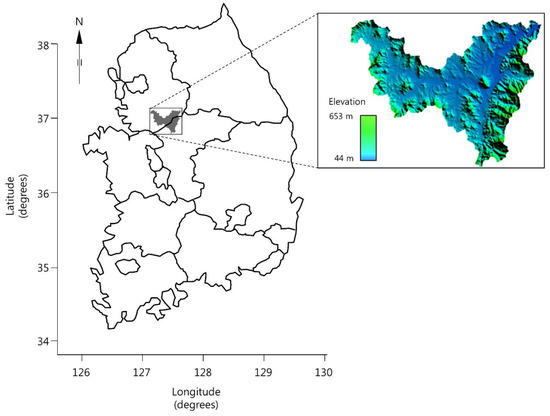
Figure 1.
Cheongmi-cheon watershed. Center is approximately 127.52° E, 37.67° N, which is about 70 km south east of Seoul, Korea.
The center of the Cheongmi-cheon watershed is approximately 127.52° E, 37.67° N, which is about 70 km east-south of Seoul, Korea. The elevation of the Cheongmi-cheon watershed is approximately 50–650 m, and the annual average temperature and humidity are approximately 11.5 °C and 66.7%, respectively. The annual average precipitation is 1184 mm, which is lower than the Korean national average of 1310 mm [23,24]. The six rain gauges are available at the Cheongmi-chen watershed and were averaged hourly and specified to simulate flow rates and stage in watershed. To assign area significance to point rainfall values, Thiessen polygons were used to apportion a point coverage into polygons. The rainfall is considered to be constant within each polygon, but each polygon has different value to give spatial distribution throughout the domain. The streamflow to compare with the simulation was collected at two points; Cheongmi station and Janghowon station, which are downstream of Cheongmi station.
The rainfall data used for this study were collected by the Korea Meteorological Administration [25], from 28 August 2012 to 1 September 2012 (5 days). The digital elevation map in this study used a modified topographic map. Contour lines and a stream channel were digitized, rasterized, and linearly interpolated [26]. The land cover map was constructed based on Landsat ETM+ reflectance data [27], and then a roughness coefficient of vegetation parameter was assigned to land cover type according to literature [28,29]. The Cheongmi-chen watershed was vegetated with about 33.2% forest mixed evergreen and broad leaf. The rest was 23.8% paddy fields and 14.7% cropland.
The soil texture data were used to specify the nature and characteristics of the surface cover, where it was compiled in the database and extracted from the Rural Development Administration of Korea [30]. The dominant soil texture of the Cheongmi-chen watershed was 59.4% well-drained sandy loam, with 17.8% loam, 17.2% silty loam, and 5.6% others. Infiltration properties that required parametrization were carried into the model parameter map according to literature [24,31].
2.2. Hydrologic Model
Given externally forcing data with surface characteristics, the flood routing processes could be handled similarly using various one- or two-dimensional routing models. The two-dimensional shallow water equations were useful mathematical formulations for describing open channels. The routing process was simulated in this study using the two-dimensional routing model, i.e., FLO-2D [31], which is a two-dimensional mechanistic model that routes runoff flood in channels. FLO-2D is a simple volume conservation flood routing model that moves the flood volume through a series of grids for overland flow or through stream segments for channel routing. FLO-2D is based on the dynamic wave of the momentum equation. FLO-2D has Green and Ampt, curve numbers and Horton equation to simulate soil infiltration [31]. The government equation for runoff and stream flow is as follows [31]:
where h is the depth of flow, V is the depth-averaged velocity in coordinate direction x, R is rainfall, and I is infiltration. The friction slope component Sf is based on the Manning equation. The other terms include the bed slope So and convective and local acceleration terms. There are many studies that show the FLO-2D’s reliability for rainfall-runoff simulation; Barnard creek mudflow alluvial fan project, Centerville, Utah, USA, California aqueduct project, Central valley, California, USA, Rogue river project, Oregon, USA, Rio Grande project, New Mexico, USA [32], The flood map updating project for the Tiber river, Rome, Italy [33]. The FLO-2D was selected for the study, because it is a test model for water resources analysis here in Korea. The U.S. Army Hydrologic Engineering Center Hydrologic Modeling System (HEC-HMS) is a one-dimensional model and includes many hydrologic analysis procedures (e.g., event infiltration, unit hydrographs, hydrologic routing). The HEC-HMS also continuously simulates evapotranspiration, snowmelt, and near-surface soil moisture. Supplemental analytical tools are provided for model optimization, forecasting streamflow, depth-area reduction, model uncertainty assessment, erosion/sediment transport, and water quality.
The Hydrologic Modeling System (HEC-HMS) is designed to simulate watershed hydrologic processes of the U.S. army Hydrologic Engineering Center [34], which is the most used practical model in Korea, because the software is freely available and simple. Lumped or semi-distributed rainfall-runoff models such as the HEC-HMS is, however, unlikely to be involved with a two-dimensional map format. The model may rely on coarsely aggregated soil geographic data in which the model needs a representative value from the two-dimensional soil parameter map. It is difficult to determine the representative value to fit the model needs; the choice is often made on a subjective and intuitive basis. The HEC-HMS features a fully integrated work environment and provides a graphical user-friendly interface. Output simulations are stored in the data storage system and are compatible with software for studies of water availability, flow forecasting, urbanization impact, reservoir spillway design, floodplain regulation, and systems operation. HMS has several options to represent infiltration losses, i.e., the curve numbers method, exponential, Green-Ampt, and Smith Parlang. Readers should refer to the HEC-HMS user manual [34] for more details.
Lumped models usually require fewer input data and have a quick run-time, and are thus easy to compare to a number of design storms. At the same time, lumped models are less detailed and they do not model changing flow directions at different flow depths. Two-dimensional distribution models are more detailed, with finer resolutions of flow conditions. Distribution models address change of flow directions at different flow depths. Therefore, it is not easy to determine a model in practice. This study provides useful guidelines on the choice of numerical averaging method to represent soil heterogeneity. We assumed that the remaining hydraulic model parameters were specified in a suitable way, and that parameters were set to be the same for all cases. A hydraulic parameter was assigned for each soil classification and a suitable integrating method for the gridded data
The value for soil-related parameters was represented on a physical basis from each grid. We considered the representative soil-related parameters to suitably capture the nature of area-averaged flow in a watershed.
Figure 2 shows the mosaic approach that assigns hydrologic parameters for each grid point. For the reasons listed above, the mosaic approach is a presumably better representation of the surface heterogeneity, and considered to be more physical.
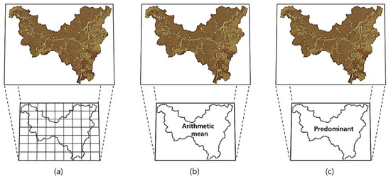
Figure 2.
Approaches to specifying hydrologic parameters: (a) mosaic, (b) arithmetic mean, and (c) predominant.
The mosaic method is a favorite of the gridded rainfall-runoff model. The arithmetic mean is a simple mathematical treatment of the representative values for the entire grid cell. The predominant approach selects the most frequent occurrence of soil type, which is equivalent to the largest portion of soil patch and defined as a representative value for the entire watershed. Three different ways described above were applied to the cell-based FLO-2D and lumped HEC-HMS model, and the hydrologic responses were compared for both the Green-Ampt and curve number, respectively.
One of the main assumptions used herein is that a model applicable at small scales can be applied at larger scales using effective parameter values.
3. Results
The Nash–Sutcliffe coefficient of efficiency (NSC) [35] and root mean square error (RMSE) were estimated to quantitatively assess the efficiency of fit between observed and estimated series of runoffs.
where and are the simulated and observed values of the discharge, respectively, and is the mean observed discharge. The index 𝑚 is the number of data points. NSC has a maximum perfect score of 1.0 and no minimum, with values greater than zero indicating that the forecasting model is better than using an arithmetic average for observations. Mathematically, NSC is one minus the ratio of the mean-square difference between observations and simulations to the variance of the observed data [35]. Both the NSC and RMSE describe the degree of association between the observed and estimated runoff. An additional measure of goodness of fit is the coefficient of determination shown in the figures.
The results of this overall modeling processes cover the generation of several hydrologic elements, including the flood hydrograph and flow routing. Discrepancies result from factors, such as spatial inhomogeneity of soil and vegetation, measurement errors, model structure errors, geomorphic effects, and land cover. The method of validation was to perform a relative comparison of the existing records and estimated values. In field environments, measurement errors are inherent in recorded data, and inadequacies may arise in subsequent simulations.
3.1. Application of the Curve Number Method
The portion percentage of assorted soil textures and corresponding parameters for the curve number method is shown in Table 1.

Table 1.
Portion percentage of assorted soil textures and the corresponding parameters for the averaged curve number.
The curve number of type II was 65 for the arithmetic method and 48 for the predominant method. The curve number in the map is redistributed in the arithmetic method, which is never seen in the predominant method. Accordingly, we investigated a relative comparison of the models for different methods of integrating soil heterogeneity against field measurements. To do this, we ran both a distributed and lumped hydrologic model to simulate the streamflow in a small watershed. Figure 3 shows the runoff and the time to reach peak flow, which is important in flood forecasting and water resource management.
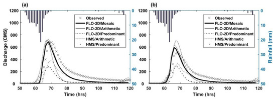
Figure 3.
Observations compared to simulations of FLO-2D and hydrologic engineering center hydrologic modeling system (HEC-HMS), based on the curve number method: (a) Janghowon, (b) Cheonmi.
Figure 3a presents the simulated streamflow via both hydrologic models at Janghowon, which is downstream of Cheongmi. Visually, we found that the streamflow simulated by FLO-2D using the mosaic method showed good performance. As shown in Table 2, the RMSE, NSC, and FLO-2D coefficient of determination using the mosaic method at Janghowon (Chengmi) were 69.6 (48.80) m3/s 0.89 (0.90), and 0.94 (0.95), respectively (see Figure 4).
Table 2.
Basic statistics for each method simulated by both FLO-2D and HEC-HMS at Cheongmi station.
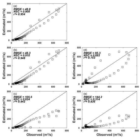
Figure 4.
Observations versus simulations using the curve number method: (a) mosaic/FLO-2D, (b) arithmetic/FlO-2D, (c) predominant/FLO-2D, (d) arithmetic/HEC-HMS, and (e) predominant/HEC-HMS.
The RMSE, NSC, and FLO-2D coefficients of determination using the arithmetic mean at Janghowon (Chengmi) were 63.24 (48.30) m3/s, 0.89 (0.91), and 0.94 (0.95), respectively. The basic FLO-2D statistics using the arithmetic mean showed slightly better performance due to a better match during early rainfall. However, the peak streamflow simulated by FLO-2D using the arithmetic mean was about 3% larger than the mosaic method. The performance was poorer in the HEC-HMS. The peak streamflow of HEC-HMS using the arithmetic method occurred earlier. The RMSE, NSC, and FLO-2D coefficient of determination using the arithmetic method at Janghowon (Chengmi) were 118.46 (95.31) m3/s, 0.64 (0.69), and 0.78 (0.75), respectively. The front arrival time and time to peak discharge showed similar behavior to peak discharge. The front arrival time simulated by the FLO-2D using the mosaic and arithmetic means at both Janghowon and Chengmi was behind the observation but time to peak discharge was close to the observation. The simulation by the FLO-2D using the predominant method at both stations had the best performance for front arrival time in relative terms. The volume simulated by the FLO-2D using the mosaic mean at Janghowon (Chengmi) was underestimated by about 7.2% (5.9%). The FLO-2D coefficient of determination using the arithmetic mean at Janghowon (Chengmi) was underestimated by about 5.8% (4.2%).
The streamflow simulated by both the FLO-2D and HEC-HMS using the predominant method was away from the observed, and attributed to the fact that the study site’s dominant soil texture was sandy loam and thus the site was highly permeable. This implied that the results were significantly different depending on the representation approach in the streamflow simulation using the hydrologic model.
Engineers and hydrologists have questioned the physical basis of the curve number method, and we found that a main limitation was the failure to account for the temporal variation in rainfall and runoff.
3.2. Application of Green-Ampt
The Green-Ampt equation was more physical and complex than the curve number method, and the governing equation for the curve number relationship was an analytical solution to the Richards equation for a simplified case [1]. The hydraulic conductivity and soil suction for the Green-Ampt equation were 8.1 mm/h and 114 mm for the arithmetic method, while being 8.1 mm/h and 109 mm for the predominant method. Portion percentage of assorted soil textures and corresponding parameters for the entire domain is shown in Table 3.
Table 3.
Portion percentage of soil classification and the corresponding parameters for Green-Ampt.
Both a distributed hydrologic model and a lumped hydrologic model were set up to simulate the streamflow and examine how different representations of soil parameters affect the simulation of a small watershed. Figure 5a,b present the streamflow simulated by FLO-2D and HEC-HMS at Janghowon and Cheongmi. The mosaic method showed better basic statistics, indicating that the streamflow simulated by FLO-2D using the mosaic method had better performance.
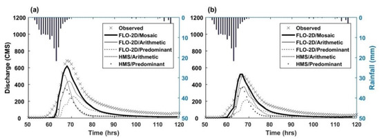
Figure 5.
A time series of the model output simulated by both the FLO-2D and HEC-HMS against the observed, using the Green-Ampt: (a) Janghowon, (b) Cheonmi.
As shown in Figure 6, the RMSE, NSC, and FLO-2D coefficient of determination using the mosaic method at Janghowon (Chengmi) were 36.6 (56.1) m3/s, 0.90 (0.87), and 0.96 (0.96), respectively.
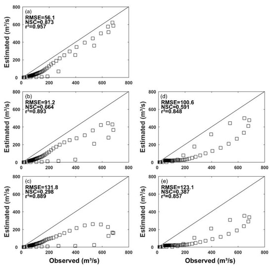
Figure 6.
Observations versus simulations using the Green-Ampt: (a) mosaic/FLO-2D, (b) arithmetic/FLO-2D, (c) predominant/FLO-2D, (d) arithmetic/HEC-HMS, and (e) predominant/HEC-HMS.
The RMSE, NSC, and FLO-2D coefficient of determination using the arithmetic method at Janghowon (Chengmi) were 58.9 (91.1) m3/s, 0.75 (0.66), and 0.96 (0.89), respectively. The peak streamflow simulated by the FLO-2D using the arithmetic mean was underestimated by about 25% against the observation, as seen in Figure 5. The front arrival time simulated by the FLO-2D using the mosaic at both Janghowon and Chengmi was behind the observation, but time to peak discharge was close to the observation. The volume of the simulated event was also related to the flood generation, infiltration losses, and propagation of the superficial runoff. The volume simulated by the FLO-2D using the mosaic at Janghowon (Chengmi) was underestimated by about 7.4% (6.2%), and when using the arithmetic mean at Janghowon (Chengmi), it was underestimated by about 9.3% (7.5%).
The performance by the HEC-HMS was similar to that in the curve number method. The peak streamflow by the HEC-HMS using the arithmetic mean was just 5% smaller against the observation at Janghowon, while it was about 10% larger against the observation at Cheonmi. However, the peak streamflow by the HEC-HMS using the predominant method was underestimated due to high permeability.
On the basis of the results, the mosaic method seemed to provide better performance, in terms of both the amount and timing in the distributed FLO-2D model. The results suggested that the arithmetic method was safer than the predominant method in the HEC-HMS.
4. Conclusions
This study examined the impact of different representations for soil-related parameters on rainfall-runoff simulations. A two-dimensional distributed rainfall-runoff model, FLO-2D, was setup in a small watershed in the Korean Peninsula, using three different methods of parameter representation. The lumped rainfall-runoff simulation and HEC-HMS were compared with both the observed and FLO-2D simulation. Two different water abstractions, curve number equivalence, and Green-Ampt were selected for in-depth investigation. The model results showed noticeable differences depending on the representation method. The mosaic method showed better representation for both the curve number and Green-Ampt. As for the mosaic approach at Chengmi, the RMSE, NSC, and FLO-2D/curve number coefficient of determination were 48.8 m3/s, 0.91, and 0.95, respectively, while the RMSE, NSC, and the FLO-2D/Green-Ampt coefficient of determination were 56.1 m3/s, 0.87, and 0.96, respectively. The time to peak discharge was close to the observation, but the front arrival time was behind the observation. However, the peak streamflow simulated by the HEC-HMS showed about a 25% discrepancy against the observation, depending on the representation method. The arithmetic mean showed better performance than the predominant method, due to the greater permeability of the dominant soil type in the watershed. Spatial variability of nonhomogeneous catchment parameters was disregarded in the lumped models, while each cell had distinct surface parameters in the distributed models. For the study region, the mosaic method was recommended for distributed models, and the arithmetic mean was recommended for lumped models. It could be a general indication that the mosaic approach was a priority when assigning soil-related parameters in distributed hydrologic models.
In some cases, a limited evaluation of the agreement between the computed and observed streamflow may be insufficient for drawing strong conclusions. The examination herein is limited, but provides useful guidelines for improving the description of soil heterogeneity and eventually, the prediction of flow in land surface processes. The method can extend to other regions for spatial distributed data manipulation in the near future. The specific results might vary depending on the classifications of general nature and soil texture, model type, surface characteristics, and rainfall magnitude effects.
The grid size of the distributed models had a considerable effect on the outflow hydrograph, having an influence on the results in terms of water depth, flow velocity, and discharge. The grid size of 50 m was used for the study. Spatial heterogeneity affected hydrologic response with variability, discontinuity, and hydrologic connectivity. Grid-based models were widely used in simulating hydrologic processes, and a prescribed single value was assigned for each grid, to represent terrain features, model parameters, and input/output variables. There is a general tendency to presume that high resolution improves the realism of surface heterogeneity for natural systems, as well as the corresponding model’s predictive ability. High resolution may improve modeling accuracy, which could increase the preparation effort and subsequent computational effort. On the other hand, large grid size may result in an inadequate representation of surface characteristics and poor modeling results. However, coarser grid cell resolutions can be used for runoff simulations, as long as parameters are appropriately calibrated. Grid size is subject to the modeler choice and experience. Caution needs to be taken.
Other sources of uncertainties such as antecedent soil moisture, rainfall intensity/duration, watershed size, soil depth, and seasonal characteristics are also likely to be important, but these details are independent of the present paper. One method to reduce uncertainties is to calibrate the parameters by using locally gaged data.
Author Contributions
Software, J.H. and H.L.; formal analysis, K.L.; validation, K.L.; writing, K.L.; visualization, J.H. and H.L. Funding acquisition, K.L. All authors have read and agreed to the published version of the manuscript.
Funding
This work was funded by a grant from the National Research Foundation of Korea (NRF-2017-2017001809).
Conflicts of Interest
The authors declare no conflict of interest. The funders had no role in the design of the study; in the collection, analyses, or interpretation of data; in the writing of the manuscript, or in the decision to publish the results.
References
- Maidment, D.R. Handbook of Hydrology; McGraw-Hill: New York, NY, USA, 1993. [Google Scholar]
- Arain, M.A.; Michaud, J.D.; Shuttleworth, W.J.; Dolman, A.J. Testing of vegetation parameter aggregation rules applicable to the Bioshpere-Atmosphere Transfer Scheme BATS at the FIFE site. J. Hydrol. 1996, 177, 1–22. [Google Scholar] [CrossRef]
- Shuttleworth, W.J. Combining remotely sensed data using aggregation algorithms. Hydrol. Earth Syst. Sci. 1998, 2, 149–158. [Google Scholar] [CrossRef]
- Lee, K. Integrating remotely sensed data using a simple vegetation parameter aggregation method applicable to a distributed rainfall-runoff model. J. Hydrol. Eng. ASCE 2008, 13, 236–241. [Google Scholar] [CrossRef]
- Griensen, A.; Bauwens, W. Identification of Distributed Parameters in Hydrologic Models, International Workshop on Catchment Scale Hydrologic Modeling and Data Assimilation; Wageningen University: Wageningen, The Netherlands, 2001. [Google Scholar]
- Koster, R.D.; Suarez, M.D. A comparative analysis of two land surface heterogeneity representations. J. Clim. 1992, 5, 1379–1390. [Google Scholar] [CrossRef]
- Kabat, P.; Hutjes, R.W.A.; Feddes, R.A. The scaling characteristics of soil parameters: From plot scale heterogeneity to subgrid parameterization. J. Hydrol. 1997, 190, 363–396. [Google Scholar] [CrossRef]
- Batjes, N.H. Soil Parameters for the Soil Types of the World for Global Use and Regional Models. International Soil Reference and Information Center (ISRIC) Report; Wageningen University: Wageningen, The Netherlands, 2002. [Google Scholar]
- Jhorar, R.K. Estimation of Effective Soil Hydraulic Parameters for Water Management Studies in Semi-Arid Zone; Wageningen University: Gelderland, The Netherlands, 2002. [Google Scholar]
- Fraga, I.; Cea, L.; Puertas, J. Effects of rainfall uncertainty on the performance of physically based rainfall-runoff models. Hydrol. Process. 2019, 33, 160–173. [Google Scholar] [CrossRef]
- Costabile, P.; Costanzo, C.; Bartolo, S.D.; Gangi, F.; Macchione, F.; Tomasicchio, G.R. Hydraulic Characterization of River Networks Based on Flow Patterns Simulated by 2-D Shallow Water Modeling: Scaling Properties, Multifractal Interpretation, and Perspectives for Channel Heads Detection. Water Resour. Res. 2019, 55, 7717–7752. [Google Scholar] [CrossRef]
- Monnar, D.K.; Julien, P.Y. Grid-Size Effects on Surface Runoff Modeling. J. Hydrol. Eng. ASCE 2000, 5, 8–16. [Google Scholar]
- Singh, V.P.; Woolhhiser, D.A. Mathematical Modelong of Watershed Hydrology. J. Hydrol. Eng. ASCE 2002, 7, 270–292. [Google Scholar] [CrossRef]
- Kim, B.; Sanders, B.F.; Schbert, J.S.; Famiglietti, J.S. Mesh type tradeoffs in 2D hydrodynamics modeling of flooding with a Gogunov-based flow solver. Adv. Water Resour. 2014, 68, 42–61. [Google Scholar] [CrossRef]
- Habtezion, N.; Nasab, T.; Chu, X. How does DEM resolution affect microtopographic characteristics, hydrologic connectivity, and modelling of hydrologic processes? Hydrol. Process. 2016, 30, 4870–4892. [Google Scholar] [CrossRef]
- Bout, B.; Jetten, V.G. The validity of flow approximation s when simulating catchment-integrated flash floods. J. Hydrol. 2018, 556, 674–688. [Google Scholar] [CrossRef]
- Ferraro, D.; Costabile, P.; Costanzo, C.; Petaccia, G.; Macchione, F. A special analysis approach for a priori generation of computational grids in the 2-D hydrodynamic-based runoff simulations at a basin scale. J. Hydrol. 2020, 582, 124508. [Google Scholar] [CrossRef]
- Fernandez-Pato, J.; Garcia-Navarro, P.; Luis-Garcia, J. A fractional-order infiltration model to improve the1 simulation of rainfall/runoff in combination with a 2D2 Shallow Water model. J. Hydroinform. Available online: https://www.researchgate.net/publication/324385619 (accessed on 11 April 2018).
- Ni, Y.; Cao, Z.; Liu, Q.; Liu, Q. A 2D hydrodynamic model for shallow water flows with significant infiltration losses. Hydrol. Process. 2020, 34, 2263–2280. [Google Scholar] [CrossRef]
- Frenandez-Pato, J.; Caviedes-Voullieme, D.; Garcia-Navarro, P. Rainfall/runoff simulation 2D full shallow water equations: Sensitivity analysis and calibration of infiltration parameters. J. Hydrol. 2016, 536, 496–513. [Google Scholar] [CrossRef]
- David, A.; Schmalz, B. Flood hazard analysis in small catchments: Comparison of hydrological and hydrodynamic approaches by the use of direct rainfall. Flood Risk Management. J. Flood Risk Manag. 2020. [Google Scholar] [CrossRef]
- Cornelissen, T.; Diekkruger, B.; Giertz, S. A comparison of hydrological models for assessing the impact of land use and climate on discharge in a tropical catchment. J. Hydrol. 2013, 498, 221–236. [Google Scholar] [CrossRef]
- MOLIT (Ministry of Land, Infrastructure and Transport). Field Survey Report 2008: Hangang Discharge; MOLIT: Seoul, Korea, 2009. (In Korean) [Google Scholar]
- MOLIT (Ministry of Land, Infrastructure and Transport). User’s Guideline to Design Flood; MOLIT: Seoul, Korea, 2012. (In Korean) [Google Scholar]
- KMA (Korea Meteorological Administration). Weather Information. Available online: http://www.kma.go.kr (accessed on 23 October 2019).
- NGII (National Geographic Information Institute). Platform of National Space Information. (In Korean). Available online: http://map.ngii.go.kr/ms/map/NlipMap.do# (accessed on 23 October 2019).
- ME (Ministry of Environment). Spatial Information Service for Environment (in Korean). Available online: http://egis.me.go.kr/map/map.do?type=land (accessed on 23 October 2019).
- Engman, E.T. Roughness coefficient for routing surface runoff. J. Irrig. Drain. Eng. 1986, 1121, 39–53. [Google Scholar] [CrossRef]
- Vieux, B.E.; Cui, Z.T.; Caur, A. Evaluation of a physio-based distributed hydrologic model for flood forecasting. J. Hydrol. 2004, 298, 155–177. [Google Scholar] [CrossRef]
- RDA (Rural Development Administration). National Institute of Agricultural Science. Available online: http://soil.rda.go.kr (accessed on 23 October 2019).
- FLO-2D Software Inc. FLO-2D, Reference Manual; FLO-2D Software Inc.: Nutrioso, AZ, USA, 2009. [Google Scholar]
- FLO-2D Pro. Available online: https://flo-2d.com/flo-2d-pro/12 (accessed on 1 January 2020).
- FLO-2D Europe. Available online: https://www.flo-2deurope.com/en/ (accessed on 1 March 2016).
- Scharffenberg, W.A.; Fleming, M.J. Hydrologic Modeling System HEC-HMS User’s Manual; U.S Army Corps of Engineers Hydrologic Engineering Center: Davis, CA, USA, 2010.
- Nash, J.E.; Sutcliffe, J.V. River flow forecasting through conceptual models, I-A discussion of principles. J. Hydrol. 1970, 10, 282–290. [Google Scholar] [CrossRef]
© 2020 by the authors. Licensee MDPI, Basel, Switzerland. This article is an open access article distributed under the terms and conditions of the Creative Commons Attribution (CC BY) license (http://creativecommons.org/licenses/by/4.0/).