Design Aspects, Energy Consumption Evaluation, and Offset for Drinking Water Treatment Operation

Abstract

Drinking water treatment, wastewater treatment, and water distribution are energy-intensive processes. The goal of this study was to design the unit processes of an existing drinking water treatment plant (DWTP), evaluate the associated energy consumption, and then offset it using solar photovoltaics (PVs) to reduce carbon emissions. The selected DWTP, situated in the southwestern United States, utilizes coagulation, flocculation, sedimentation, filtration, and chlorination to treat 3.94 m³ of local river water per second. Based on the energy consumption determined for each unit process (validated using the plant’s data) and the plant’s available landholding, the DWTP was sized for solar PV (as a modeling study) using the system advisor model. Total operational energy consumption was estimated to be 56.3 MWh day⁻¹ for the DWTP including water distribution pumps, whereas energy consumption for the DWTP excluding water distribution pumps was 2661 kWh day⁻¹. The results showed that the largest consumers of energy—after the water distribution pumps (158.1 Wh m⁻³)—were the processes of coagulation (1.95 Wh m⁻³) and flocculation (1.93 Wh m⁻³). A 500 kW PV system was found to be sufficient to offset the energy consumption of the water treatment only operations, for a net present value of $0.24 million. The net reduction in carbon emissions due to the PV-based design was found to be 450 and 240 metric tons CO₂-eq year⁻¹ with and without battery storage, respectively. This methodology can be applied to other existing DWTPs for design and assessment of energy consumption and use of renewables.

1. Introduction

Energy conservation and sustainability is one of the pressing issues being faced by the water industry today as drinking water treatment and wastewater treatment are highly energy-intensive processes [1]. These processes account for about 2% of the United States’ total energy use, resulting in the emissions of about 45 million tons of greenhouse gases (GHG) [2]. One of the ways to reduce carbon emissions is to incorporate renewables into existing water infrastructure. The objective of this study was evaluation of the energy consumption of a large-scale drinking water treatment plant (DWTP), associated carbon emissions, and then offsetting that energy consumption by utilizing photovoltaics (PVs).

Energy use related to drinking water treatment may include energy for water conveyance, energy for unit operations of the DWTP, for facility related equipment (lighting, heating and ventilation), and energy for water distribution [3,4]. Energy use for water treatment depends on various factors such as raw water quality, water source, age of water delivery system, conveyance distance, water storage capacities, as well as elevation differences. About 80% of the energy use is for conveying or pumping the water and wastewater while the remaining is used for water treatment [5].

Literature Review

Treatment of water is an energy-intensive process. Various studies have evaluated the energy consumption for drinking water treatment [6,7,8,9,10,11,12] and wastewater treatment plants [13,14,15,16,17]. More studies exist for wastewater treatment facilities compared to DWTPs. Ref. [12] conducted a literature review and compared energy consumption of a conventional water treatment in various countries including Australia (0.01–0.2 kWh m⁻³), Spain (0.11–1.5 kWh m⁻³), New Zealand (0.15–0.44 kWh m⁻³), U.S. (0.184–0.47 kWh m⁻³), Canada (0.38–1.33 kWh m⁻³), and Taiwan (0.16–0.25 kWh m⁻³). Similar studies were also conducted by [9]. Ref. [8] determined the energy consumption of a DWTP, treating 0.017 m³ day⁻¹ of river water, located in Jamshoro Pakistan, as 7.4 Wh m⁻³. The largest consumers of energy were the processes of chlorination (because of on-site generation of chlorine dioxide) and coagulation, consuming about 34% and 31% of the total operational energy consumption of the DWTP. Ref. [11] studied the effects of mixing intensity on floc formation as well as the associated energy consumption.

Future energy demands related to water treatment are expected to grow because of various reasons. Energy expenditure of water operations increases due to population growth [18,19,20,21,22] as well as aging infrastructure [23]. Further, pollution is caused by emission of GHG, due to the burning of carbon-based fuels for electricity generation [24]. These can be motivating factors for DWTPs to explore and implement different methods to reduce their overall energy consumption. Changing climate complicates the matter further [25,26,27,28,29,30,31,32,33,34]. Changes in temperature and increased drought/flood conditions may result in the degradation of source water [35,36,37,38,39]. Furthermore, in recent times, with technological advancement and introduction of new chemicals into the environment, there has been an increased emphasis on stringent water quality standards [40,41,42], enforced by the implementation of various regulations [43], although enforcement of such standards may not be possible today because of the high costs of treatment associated with it [44]. Employing alternate ways to generate energy such as using renewables or using energy conservation measures can help in cost reduction [23].

Renewable energy resources including solar, wind, and biomass can be used to generate energy for water systems, including drinking water and wastewater treatment processes and water pumping and supply. This will lead to a decrease in fossil fuel-based energy requirements. Solar energy is gaining popularity as a clean source of energy production. Sunlight is an abundant resource, especially in the southwest, and application of this technology may help towards energy independence as well as reduction in GHG emissions, as during operation, solar energy has zero carbon emissions, but there are some emissions generated during construction and transportation of solar technologies [45].

Solar PVs generate electricity by converting sunlight directly into electricity by utilizing the photoelectric effect and the photovoltaic effect. Using PV has an additional advantage of being able to supply balanced and sustainable power throughout the day, even at the time of peak demand when electric power is the most costly. Solar PV can be deployed at utility, commercial, and residential scale and as decentralized or grid-connected systems [46].

Deployment of solar energy depends on financial viability since it entails large capital costs, recurring costs for operation and maintenance (O&M), and government taxes paid over the life of the project [47,48]. Different governmental incentives and policies help dissipate these costs and assist in making solar energy economically competitive with other sources of energy generation [49]. The costs associated with solar installations can also be dissipated indirectly due to the corresponding reduction in carbon emissions, leading to improved health of the community and the environment [50,51].

Application of PV depends on land availability, and deployment requires a large land area [45,52]. PV can be ground-mounted or installed on rooftops. Drinking water treatment plants are usually located upstream of the community they serve while wastewater plants are located downstream of the community and are provided with sufficient land acreage based on anticipated future development and redevelopment. The existing landholdings of the treatment plant can be utilized for the installation of solar energy [53,54]. If the landholdings of the treatment plant are not sufficient, then additional land area would need to be acquired.

Design and performance analysis of solar PV can be achieved using available modeling tools. The system advisor model (SAM) developed by the National Renewable Energy Laboratory in 2005 [55] is a performance and cost-modeling tool and facilitates in decision making for renewables of solar, wind, and geothermal and biomass combustion. Various studies have used SAM for analyzing solar technologies, particularly photovoltaics [56,57,58,59]. Ref. [59] utilized SAM to generate hourly performance simulations for the validation of their solar PV design. Solar PV was used to generate power for the aerators, utilized for the treatment of acid mine drainage at Hwangji Youchang facility, located in Korea. The 30.1 kW PV system, using a factor of safety of 5, resulted in electricity production of 3016 kWh month⁻¹, to meet the 342.39 kWh month⁻¹ electricity demand [59]. Ref. [56] utilized SAM to generate life cycle costs per kWh for utility-scale development of solar PV as well as for using solar PV to meet the electricity demands for residential and commercial sectors in the United States. Ref. [58] employed SAM for analyzing life cycle energy production and associated costs of a solar PV system and solar water heater for a residential dwelling unit in Houston, Texas.

Solar energy has great potential as a clean source of energy for water treatment processes [7,60,61,62], wastewater treatment processes [63,64,65,66], and desalination [67,68,69,70,71]. Studies evaluating the potential of existing DWTPs to incorporate solar energy technologies are limited. Ref. [61] made performance comparisons between a conventional DWTP and a wind-solar-powered nano-filtration pilot plant located in Spain. Ref. [62] explored the potential of using wind and solar energy for a large-scale water treatment plant in the Netherlands. The goal of this study was to:

(a)

Design and determine the energy consumption and energy intensity of each unit operation (validated using plant’s data) of an existing DWTP,

(b)

Conduct a modeling study and size the DWTP for solar PV, to offset the energy consumption of the plant, based on available landholdings and economic assessment,

(c)

Determine the net reduction in carbon emissions due to solar PV installation compared to non-PV based design.

The approach used in this study can be utilized as a guide to design DWTPs and analyze their energy consumption. This is useful for engineers and researchers as generally consulting firms do not publicly disclose such information. For a meaningful design, data was collected from an existing DWTP. Further, sustainability is incorporated into the design of the plant by using solar PV, with the long-term goal of energy independence and reduced carbon emissions for an existing DWTP.

2. Study Area

For this study, the selected treatment plant is located in southwestern United States, serving a city with a population of 0.24 million. The primary water supply for the city is a river originating from a lake, enduring a 161 km course through different canyons and ultimately having an outfall in another lake. Only 6% of the water flowing through the river is used by the community, and in addition, almost half of that 6% is returned to the river after the generated wastewater is treated at the wastewater treatment plants. Hence, only 3% of the water flowing through the river is used in a non-drought year, while 8% is used in a drought year. The DWTP has the capacity to treat 3.94 m³ of source water per second. For confidentiality reasons, the location of the plant cannot be disclosed, as required by the DWTP’s management, since data was collected from the DWTP’s managers for validation of the results generated in this study. However, for the purpose of analysis of the PV system, it was assumed that the plant was located in Nevada (direct beam insolation level 6.3 kWh m⁻² day⁻¹), having insolation levels favorable for solar deployment.

3. Data Sources

Data sources for this study are as follows:

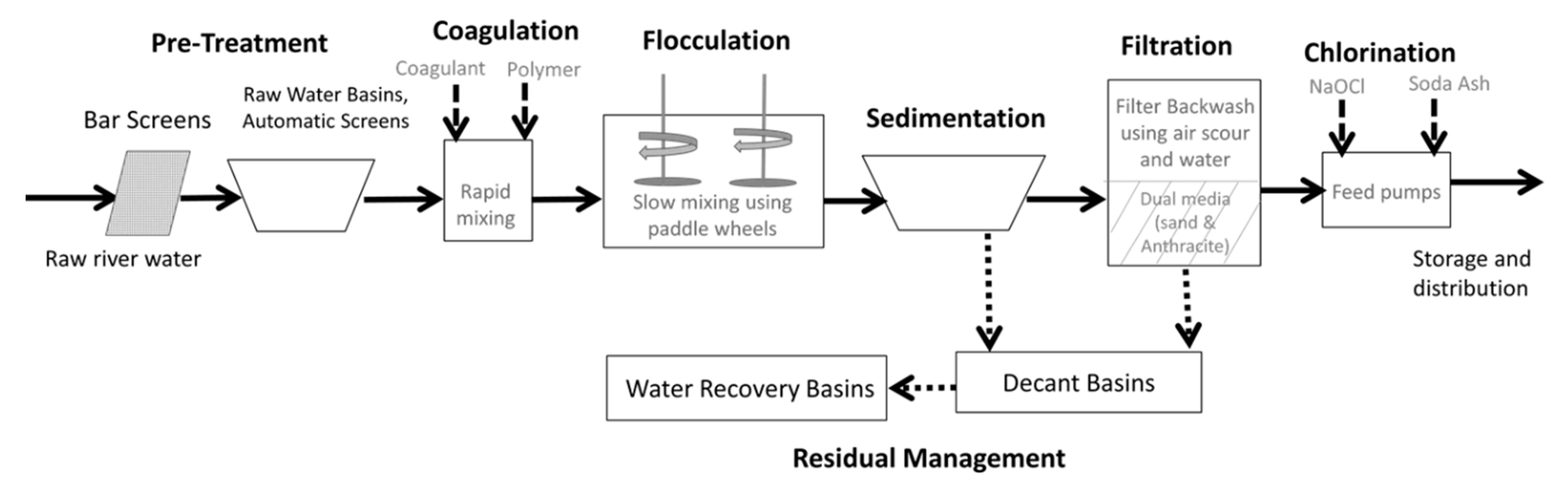
3.1. Process Flow Diagram

A process flow diagram was acquired from the treatment plant managers. The process flow diagram discussed in this section for the DWTP is based on the information provided.

Figure 1 shows the process flow diagram for the plant, which utilizes a conventional treatment train to treat 3.94 m³ of river water per second. Raw water from the river at first undergoes pre-treatment and passes through bar screens, raw water basins, and then automatic screens for removal of larger debris, settlement of heavier grit, and removal of smaller debris, respectively. Then, the water is coagulated and flocculated. Next, the water is filtered through dual-media filters. Lastly, the water is disinfected by application of sodium hypochlorite and then stored for distribution throughout the city.

3.2. Water Quality Report

A raw water quality report was acquired from the DWTP’s managers, and any missing data was reproduced from [43]. The design for each unit process is dependent upon the raw water characteristics as well as the corresponding maximum contaminant levels (MCL) and secondary maximum contaminant levels (SMCL) determined by the U.S. Environmental Protection Agency (USEPA), as shown in

Table 1. Raw water quality report obtained from the drinking water treatment plant’s managers.

Parameter	Units	Average Value	USEPA* MCL **/SMCL *** Guidelines
pH	N/A	8.2	6.5–8.5
Water temperature (winter)	°C	5	Not regulated
Water temperature (summer)	°C	19	Not regulated
Turbidity	NTU	4	0.3

* USEPA: U.S. Environmental Protection Agency. ** MCL: maximum contaminant level. *** SMCL: secondary maximum contaminant level.

[72].

3.3. Treatment Plant Design Criteria

Sizing was achieved by using industry accepted design criteria [43,73,74,75] and discussed in detail in Section 4.

3.4. Carbon Emissions

Data sources and parameters for carbon dioxide emissions and southwestern state’s energy-source mix for electricity generation is shown in

Table 2. Carbon emissions [76] and Nevada’s electricity source mix [77].

Sources for Electricity Generation	Carbon Emissions (gCO2eq kWh−1)	State Electricity Source Mix
Coal	1001	23.51
Natural Gas	469	56.41
Petroleum	840	0.07
Nuclear	16	0
Hydropower	4	7.42
Bio-power	18	0.1
Geothermal	45	8.5
Wind	12	0.95
Solar	46	3.04

. Carbon emissions data in units of gCO₂-eq kWh⁻¹, for different energy sources for electricity generation, was obtained from [76]. Nevada’s electricity source mix for various energy sources was obtained from U.S. Energy Information Administration (USEIA) [77].

3.5. PV System

Parameters used for sizing solar PV, related to the PV module, inverter, and battery storage are shown in

Table 3. Photovoltaic system design parameters utilized as inputs in system advisor model [78,79,80].

	Parameter	Unit	Value
Module	Module Name	-	Helio USA 7T2 305
	Module Area	m2	1.952
	Module Material	-	Mono C-Si
	Nominal Efficiency	%	15.6
	Maximum Power Pmp	Watt	305
	Maximum Power Voltage Vmp	Volt	36.7
	Maximum Power Current Imp	Ampere	8.3
	Open Circuit Voltage Voc	Volt	45.1
	Short Circuit Voltage Isc	Ampere	8.9
Inverter	Inverter Name	-	Fronius-Symo 10.0-3 240V
	Weighted Efficiency	%	96.5
	Maximum AC Power	Watt	9995
	Maximum DC Power	Watt	10,359
	Nominal AC Voltage	Volt	240
	Maximum DC Voltage	Volt	600
	Maximum DC Current	Ampere	41.5
	Minimum MPPT DC Voltage	Volt	300
	Nominal DC Voltage	Volt	371.6
	Maximum MPPT DC Voltage	Volt	500
Battery	Name	-	Lead Acid Flooded
	Cell Nominal Voltage	Volt	2
	Internal Resistance	Ohm	0.1
	C-rate of discharge Curve		0.05
	Fully Charged Cell Voltage	Volt	2.2
	Exponential Zone Cell Voltage	Volt	2.06
	Nominal Zone Cell Voltage	Volt	2.03
	Charged Removed at Exponential Point	%	0.25
	Charge Removed at Nominal Point	%	90
	Cell Capacity	Ah	1284
	Max C-rate of Charge	h−1	0.12
	Max C-rate of Discharge	h−1	0.12
	Minimum State of Charge	%	10
	Maximum State of Charge	%	95
	Minimum Time at Charge State	min	10

. The PV system was sized as 2-axis tracking and consists of a mono-crystalline silicone module assumed to be ground mounted. A 2-axis tracking system allows higher energy output compared to single-axis trackers or fixed systems. The module type selected was Helio USA 7T2 305 [78]. Inverters are used to convert the direct current output of the solar modules into alternating current, so that the generated electricity can be utilized by the DWTP or the excess generation can be utilized by the electricity grid. The inverter type selected was Fronius Symo 10.0 240V. The battery type chosen was lead acid flooded [79,80] (Table 3).

Various financial parameters incorporated within the economic model of SAM, are listed in

Table 4. Financial parameters used for economical assessment using system advisor model.

	Parameter	Unit	Nevada Values	New York Values	References
Direct Cost	Module	$ Watt−1	1.6	1.6	[78]
	Inverter	$ Watt−1	5.0	5.0	[79]
	Battery bank	$ kWh−1	157.7	157.7	[80]
	Battery bank replacement cost	$ kWh−1	112	112	[62]
	Electrical Balance of equipment cost	$ Watt−1	0.12	0.18	[82]
	2-axis-tracking equipment	$ Watt−1	0.2	0.2	[89]
	Installation labor	$ Watt−1	0.15	0.18	[82]
	Contingency	%	4.0	4.0	[82]
Indirect Cost	Permitting, environmental studies, grid interconnection	$ Watt−1	0.1	0.12	[82]
	Engineering and developer overhead	$ Watt−1	0.53	0.55	[82]
	Installer margin and overhead	$ Watt−1	0.19	0.19	[82]
O&M Cost	Fixed annual cost	$ kW−1 year−1	18	18	[82]
Financial Rates	Inflation rate	%	2.5	2.5	SAM default value
	Real discount rate	%	8.0	8.0	[85]
	Federal income tax rate	% year−1	28	28	[83]
	State income tax rate	% year−1	0.0	8.82	[90]
	Sales tax	%	8.1	4.375	[49,90]
	Insurance rate	% of installed costs	0.25	0.25	[88]
	Salvage value		20	20	[91]
	Property tax rate	% year−1	0.0	2.0	[49]

. These parameters were based upon the review of published literature in the years 2016 and 2017 [81,82,83,84,85,86,87,88].

3.6. Federal and State Incentives

Federal and state incentives were obtained from the Database of State Incentives for Renewables & Efficiency (DSIRE) [49]. These incentives were applied in this study for economic assessment. Federal investment tax credit (ITC) represents a percentage of investments that the owners are allowed to deduct from their taxes, dollar-to-dollar. Solar projects of a commercial, industrial, or agricultural nature, implemented before or during the year 2019, can claim 30% ITC, while 26%, 22%, and 10% ITC can be claimed by projects implemented during 2020, 2021, and 2022 and onwards, respectively. If federal taxes owed are less than 30% of installed costs, solar PV owners owe no taxes for that year, and any unused tax credit is carried over to the next year. A state property tax exemption incentive, applicable for the design life of solar PV, was also incorporated into the economic analysis. This incentive cannot be claimed if another state tax abatement or exemption is claimed by the same building. Therefore, only these two incentives were incorporated in the analysis.

4. Methodology

The first step of the current research focused on sizing the DWTP by designing the various unit processes involved. Sizing was achieved by using industry accepted design criteria [43,73,74]. Design of the plant and estimation of energy consumption were determined for the maximum day demand flow anticipated for the design life of the plant (3.94 m³ s⁻¹). Thus, the analysis is representative of the worst-case scenario for the DWTP. Other parameters chosen were also reflective of the extreme conditions.

Each unit process was designed and its energy driving units were identified; then, energy consumption (kWh day⁻¹ and kWh m⁻³) for each unit process (coagulation, flocculation, sedimentation, filtration, chlorination, residual management) was individually determined and validated using the plant’s data (Section 4.1). Computations were made using Microsoft Excel Spreadsheet. Next, the system advisor model (SAM) was used to conduct a modeling study to determine the techno-economic performance of using solar PV (by sizing solar PV and battery storage based on economic metrics) to offset the energy consumption of the DWTP (Section 4.2). Land requirements of the PV deployment were compared against available landholdings of the plant to check for the sufficiency of the available area for PV deployment (Section 4.3). Net reduction in carbon emissions was determined by comparing a PV-based design (modeling study) to a non-PV based design (actual plant operation) (Section 4.4).

4.1. Design and Energy Consumption for the DWTP

4.1.1. Pre-Sedimentation

Pre-sedimentation initiates suspended solids removal and equalizing of variable turbid loadings entering a DWTP. Typically, plants treating river water are equipped with raw water basins, as river water is high in turbidity [92]. Two tanks should be provided at a minimum to incorporate redundancy in the system. Surface loading rates vary between 200 and 400 m³m⁻²day⁻¹, while detention time varies between 6 and 15 min [43].

4.1.2. Coagulation

Application of a coagulant assists in destabilizing a colloidal suspension, causing collides to agglomerate and form flocs. A coagulant’s dose and type is dependent upon the results of a jar test. The selected DWTP utilized ferric sulphate Fe₂ (SO₄)₃ as a coagulant. After the coagulant is added, rapid or flash mixing ensures uniform dispersion of the coagulant throughout the basin. In this case, a static mixer was used because mixing was achieved in the conveyance pipe between the coagulant intake pipe and flocculation basin. At least two mixers should be provided. A Reynolds number >2000 implies turbulence and good coagulation performance [75]. Velocity gradient (G) remains a significant parameter for the design of mixers. The equation to compute the G value of a static mixer [75] is as follows:

$$\mathrm{G}=\sqrt{\frac{\mathrm{P}}{\mathsf{\mu }\mathrm{V}}}$$

(1)

where G = root-mean-square velocity gradient (s⁻¹), P = power imparted to water (N-m s⁻¹), V = mixer volume = product of pipe area and length of mixer (m³), and μ = dynamic viscosity (N-s m⁻²). Energy consumption (E) in the units of kWh day⁻¹ of the mixers was found using the following equation [75].

$$\mathrm{E}=\frac{({\mathrm{G}}^2)\left(\mathsf{\mu }\right)\left(\mathrm{V}\right)\left({\mathrm{t}}_{\mathrm{m}}\right)}{\mathrm{f}}$$

(2)

where t_m = motor run time (h day⁻¹), and f = motor efficiency factor. Typically, motor efficiency is in the range 0.7–0.9 [93]. For this study, a value of 0.8 was used. Since the plant operates 24 h per day, a motor run time of 24 h was used. Energy consumption of the metering pump was determined using the brake horsepower (BHP) equation [94], which is as follows:

$$\mathrm{BHP}\left(\mathrm{kW}\right)=\frac{\mathsf{\gamma }\mathrm{QH}}{\mathrm{e}}$$

(3)

where γ = specific weight (kN m⁻³), Q = flow rate (m³ s⁻¹), H = total dynamic head (m), and e = wire-to-water efficiency. Wire-to-water efficiency can be estimated as the product of pump, motor, and drive efficiency. A jet diffuser pump was used to flash-mix coagulant aid polymer. Power (P) estimations were made using following equation [75].

$$P\left(\mathrm{kW}\right)=\frac{{\mathrm{Q}\mathsf{\gamma }\mathrm{gv}}_{\mathrm{jet}}}{2\mathrm{g}}$$

(4)

where v_jet is the jet velocity emerging from the orifice (m s⁻¹), and g = acceleration due to gravity (9.81 m s⁻²). As in Equation (3), Q = flow rate, and γ = specific weight of water.

4.1.3. Flocculation

After coagulation, the flocculation process assists in the formation of flocs, which are later separated through the processes of sedimentation and filtration. In contrast to the coagulation process, which involves flash mixing to disperse the coagulant within the feed water, the flocculation process involves slow mixing to enhance the contact between the coagulant and the feed water and for the subsequent formation of flocs. Paddle wheels are used for the flocculation process (rotational speed 0.3–3 rev min⁻¹). The coagulated water flows into the flocculation basins, where flocculation is achieved in stages with varying velocity gradient (5–40 s⁻¹) [43]. The following equation was used to estimate the energy consumption of paddle wheel flocculators.

$$\mathrm{E}\left(\mathrm{kWh} {\mathrm{day}}^{-1}\right)=\frac{({\mathrm{G}}^2)\left(\mathsf{\mu }\right)\left({\mathrm{Q}}_f\right)\left({\mathrm{t}}_s\right)\left(t_m\right)\left({\mathrm{n}}_f\right)}{\mathrm{f}}$$

(5)

where n_f = number of flocculation basins, Q_f = flow rate in each flocculation basin (m³ min⁻¹), and t_s = detention time per stage (minute). The variables G, µ, f, and t_m are the same in as in Equation (2).

4.1.4. Sedimentation

After the water is coagulated and flocculated, it moves into the sedimentation basins so that heavier flocs settle out of suspension. Compared to conventional gravity sedimentation, parallel plate settlers provide enhanced solids removal capabilities in a smaller area, even during periods of extremely high solid loadings to the plant. Parallel plate sellers were designed based on the criteria provided by [43,75,95]. The energy consumer for the parallel plate settlers were sludge transfer pumps, and their brake horsepower can be estimated using Equation (3).

4.1.5. Filtration

A dual-media (anthracite and sand) filter is employed to trap the flocculated water, using a rapid filtration process, to provide a finished water quality of ≤0.3 NTU and 4 log removal of cryptosporidium. Parameters used for the filter design [74] include filtration rate (14.5 m h⁻¹), effective size of filter media (anthracite 1 mm, sand 0.5 mm), filter media depth (anthracite 1.4 m, sand 0.25 m), and net available head (1.8–3.0 m).

Typically, to arrive at the plant the water has to be pumped from the water source to the plant. For the selected DWTP, raw water flows by gravity from the river, passes through bar screens and flows by gravity through the rest of the plant. The raw water usually flows by gravity between one unit to the next, in a typical water treatment facility. In the selected plant, after undergoing the processes of coagulation, flocculation, and sedimentation, raw water flows by gravity into the filtration unit. The filtered water is chlorinated and then moved into the finished water reservoir. The energy-consuming part of the filtration process is the backwash system (backwash pumps and air scour). Air blowers operate by developing a pressure differential to move air between the entrance and exit points [75]. Air scour of the filter media was achieved for 4 min before the application of water backwash. The power estimation for the air blower was made using the following equation [96].

$$\mathrm{P}\left(\mathrm{kW}\right)=\frac{\mathrm{wRT}}{8.41\mathrm{e}}[{\left(\frac{{\mathrm{P}}_2}{{\mathrm{P}}_1}\right)}^{0.283}-1]$$

(6)

where w = air mass flow (kg s⁻¹), R = universal gas constant (kJ k⁻¹ mole °K), T = air temperature at inlet (°K), P₁ = absolute pressure at entrance (Pascal), P₂ = absolute pressure at exit (Pascal), e = efficiency = 0.8, n = (k−1) (k⁻¹ )= 0.283 for air, and 8.41 is constant for air (kg k⁻¹ mole).

The filter is backwashed when the head loss exceeds the available head or increased turbidity is displayed in the filter effluent. The backwash system was designed [43] using the data obtained from the DWTP (backwash duration 9 min, backwash frequency 24 h). The energy consumption of the backwash pumps can be determined using Equation (3).

4.1.6. Chlorination

Disinfection can be accomplished through chlorination, ultra-violet radiation treatment, or ozonation. For the DWTP, filtered water was disinfected through chlorination using sodium hypochloride (NaOCl) applied in liquid form. The chlorination design was achieved using the design criteria provided by [93,97,98,99]. The surface water treatment rule was applied for 4 log inactivation of viruses and 3 log inactivation of giardia. A minimum one-hour detention at average design flow or 30 min detention at peak hourly flow was used, whichever was greater. The energy consumers for the chlorination process were the metering pumps; the energy consumption can be determined using Equation (3). Finished water was distributed throughout the city using highly energy-intensive zone-1, zone-2, and zone-3 pumps.

4.1.7. Residual Management

Filtration backwash wastewater and sedimentation sludge generated during filtration and sedimentation is treated using decant basin and water recovery basins, designed using the same criteria as pre-sedimentation basins. At these facilities, plant waste solids are concentrated and dewatered to recover water and to facilitate ultimate solids disposal. Decanted water is recycled through the plant, while the decant basin settled solids are pumped by solids transfer pumps to water recovery basins for secondary solids settling. Dewatering of drinking water sludge will vary depending upon coagulant type used, solids loading, and pH [100].

Energy consumption was evaluated for two main scenarios for the selected treatment plant. Scenario 1 (S-1) represents analysis for the DWTP including water distribution pumps, whereas Scenario 2 (S-2) represents the analysis for the DWTP without including the water distribution pumps.

4.2. System Advisor Model

Energy consumption for each unit process of the DWTP was determined (Section 4.1) and used as an input for SAM, a modeling tool utilized to evaluate the techno-economic performance of using solar PV to offset the energy consumption of the DWTP.

4.2.1. Technical Analysis

SAM evaluates energy performance and cost for grid-connected systems based on location and system design parameters. Electric load of the DWTP, electric rate, typical meteorological year (TMY3) data of the location, as well as the parameters related to PV panels were the primary inputs for SAM. An analysis period of 25 years was used.

The energy consumption estimate determined using the steps outlined in Section 4.1 was used as an electric load input for sizing solar PV. Electricity generation by the PV system meets the facility’s electrical load that would otherwise be met by electricity from the grid and hence reduces the electric bill. Time of use (TOU) electricity rates for large general service were applied that mainly consist of energy charges, demand charges, fixed monthly charges, and facilities charges. Summer months comprised of July, August, and September, whereas the remaining months were treated as winter months. Electricity rates are different for summer and winter months. Rate charges are also based upon voltage levels categorized as secondary (≤600 V), primary (levels between 600–25,000 V), and high voltage transmission (>25,000 V). Rates for secondary voltage levels were applied for the DWTP.

The PV system was sized using SAM by using the inputs of desired array size and a DC-to-AC ratio. Using the parameters of the selected module and inverter, the number of inverters and modules were determined. Nameplate capacity was determined as the product of the module’s maximum rated power and total number of modules. Some of the equations used to size solar PV are as follows:

$${\mathrm{M}}_{\mathrm{string}}=\frac{{\mathrm{V}}_{\mathrm{mppt}-\max }+{\mathrm{V}}_{\mathrm{mppt}-\min }}{2{\mathrm{V}}_{\max }}$$

(7)

$${\mathrm{M}}_{\mathrm{parrallel}}=\frac{\mathrm{C}}{{\mathrm{I}}_{\mathrm{pmax}}{\mathrm{M}}_{\mathrm{string}}}$$

(8)

$${\mathrm{I}}_{\mathrm{n}}=\frac{({\mathrm{M}}_{\mathrm{n}})({\mathrm{M}}_{\mathrm{mp}})}{\mathrm{DC}-\mathrm{AC}\mathrm{Ratio}\left({\mathrm{I}}_{\mathrm{map}}\right)}$$

(9)

$${\mathrm{M}}_{\mathrm{n}}={\mathrm{M}}_{\mathrm{string}}\times {\mathrm{M}}_{\mathrm{parallel}}$$

(10)

where M_string = modules per string, M_parallel = module strings in parallel, V_mppt-max = maximum MPPT voltage, V_mppt-min = minimum MPPT voltage, V_max = maximum power voltage, C = array nameplate capacity (kW), I_pmax = module maximum power, I_n = number of inverters, M_mp = Module maximum power, I_map = Inverter maximum AC power, and M_n = total number of modules.

Battery storage was also provided, primarily to meet energy demands at nighttime since the treatment plant operates for 24 h per day. SAM allows the analysis of three types of batteries: lead-acid, lithium-ion, and vanadium redox flow. For this study, a lead-acid battery was used. The battery was assumed to be connected on the AC side. Battery bank size can be specified as either the number of battery cells in a series and battery strings in parallel, or it is estimated using SAM using the inputs of desired bank capacity and bank voltage.

$${\mathrm{B}}_{\mathrm{ns}}=\frac{{\mathrm{B}}_{\mathrm{dbv}}}{{\mathrm{B}}_{\mathrm{ncv}}}$$

(11)

$${\mathrm{B}}_{\mathrm{nbv}}={\mathrm{B}}_{\mathrm{ncv}}\times {\mathrm{B}}_{\mathrm{ns}}$$

(12)

$${\mathrm{B}}_{\mathrm{np}}=\frac{{\mathrm{B}}_{\mathrm{dbc}}}{{\mathrm{B}}_{\mathrm{nbv}}\times {\mathrm{B}}_{\mathrm{cc}}}$$

(13)

$${\mathrm{B}}_{\mathrm{nbc}}={\mathrm{B}}_{\mathrm{ns}}\times {\mathrm{B}}_{\mathrm{np}}\times {\mathrm{B}}_{\mathrm{cc}}$$

(14)

where B_ns = number of battery cells in series, B_dbv= desired bank voltage, B_ncv = battery nominal cell voltage, B_nbv = nominal bank voltage, B_np = number of battery strings in parallel, B_cc = battery cell capacity, B_nbc = nominal bank capacity, and B_{db c}= desired bank capacity.

Nominal cell voltage was the manufacturer reported voltage (volt) of a single cell in a battery, which was used to size the battery storage. C-rate governed the charge and discharge rate of the battery. Max C-rate of charge and discharge of 0.12 per hour was used. SAM utilized a lifetime model that considered battery charge cycles as the main reason for capacity degradation. Capacity degradation was simulated as a function of depth of discharge and number of charge cycles, where depth of discharge described the state of the battery’s remaining charge. The capacity losses were incorporated into the maximum battery capacity after each charge cycle had elapsed. SAM does not incorporate the thermal behavior of the battery into the lifetime model; hence, it was assumed that the battery was stored in an air-conditioned room, at constant temperature.

4.2.2. Financial Analysis

Economic performance was analyzed using SAM by employing the parameters of net present value (NPV) and levelized cost of electricity (LCOE). NPV for a system examines the difference between the present value of revenues and costs. A positive NPV means that the present expenses incurred are predicted to provide a return greater than the initial investment. If the NPV is negative, then the cash inflows are predicted to be less than the cash outflows and the investment is not financially beneficial. LCOE was also estimated, which is the present value of the life cycle cost of the PV system. Real LCOE is adjusted for inflation, whereas nominal LCOE is not. Net savings in $ year⁻¹ are estimated by taking the difference between the costs for purchased electricity, with and without the solar system. For this study, NPV was used as the primary metric for financial assessment of the PV system. This is because the analysis includes the input parameters of taxes and incentives, which may complicate the estimation of more simplistic metrics such as payback period. In addition, payback period is not recommended when investment is to be considered explicitly. NPV gives value to the size of investment, while the metrics of LCOE and payback period do not [101].

Various financial parameters incorporated within the economic model of SAM are listed in Table 4, while others are discussed in the following sections. An analysis period of 25 years was used based upon the warranty period of the PV panels.

Net capital cost of the solar system was calculated using SAM, by subtracting cash incentives from total installed costs (sum of direct and indirect cost) (Table 4). Annual costs incurred for the operation, maintenance, and repairs of the solar system, after it has been installed, constitute the O&M cost ($18 kW⁻¹ year⁻¹), which increased each year based on the inflation rate for this analysis. Any savings through the application of state or federal incentives was also taxable. Savings achieved due to the installation of a solar system were not taxable; however, O&M costs were taxable. Debt percentage, which is a fraction of the net capital costs, was specified as 100%, and the debt payments were assumed constant. Principal amount was estimated using SAM as the product of total installed cost and debt percentage. A loan term of 25 years and interest rate of 3.5% were used as inputs to SAM [87]. Salvage values were taken as 20% of installed costs [91].

If land required for installation of a PV system needs to be purchased, the land cost can be incorporated in SAM’s financial model. This study assumed that the existing empty land acreage of the treatment plant would be utilized for the installation of the PV system. Hence, land purchase costs were taken as zero.

In SAM, the inflation rate (2.5%) applied to the system costs, electricity rates, and cash incentives, among others, was the yearly mean consumer price index data between the years 1991 and 2012. The real discount rate (8%) is the nominal discount rate minus the inflation rate and is used for the estimation of NPV and LCOE using SAM. In SAM, yearly insurance cost and property tax cost is tax deductible for commercial projects and is a component of the annual operating costs. The insurance rate was taken as 0.25% of the installed costs [88]. For the first year, the insurance amount was a product of the insurance rate and total installed cost, which is then increased by an inflation rate of 2.5% for later years. The property tax amount is the product of the property tax rate and assessed value of the property. The property tax rate was taken as zero to incorporate the property tax exemption incentive.

Depreciation reduces the federal and state taxable income. Different depreciation methods are available. Sometimes the method used to estimate depreciation is dictated by the Federal Government or the state. MACRS (modified accelerated cost recovery system), a depreciation method to help recover capital costs and reduce tax liability, was utilized for this analysis since qualifying systems are those that claim the 30% ITC. Commercial PV is eligible to depreciate over a five-year period [49] as determined by the Internal Revenue Service at depreciation rates of 20%, 32%, 19.2%, 11.52%, 11.52%, and 5.76% for year 1, 2, 3, 4, 5, and 6, respectively. The renewable energy system’s taxable basis can be reduced by one half of the investment tax credit of 30%, hence 85% of the taxable basis can be reduced. A bonus depreciation of 50%, 40%, and 30% can be further applied for PV systems placed in service before the year 2018, during 2018, and during 2019, respectively.

Sales tax amount was estimated as the product of sales tax % and direct cost. Since SAM incorporates the sales tax amount as a part of the total installed costs of the solar system, the sales tax amount influences the estimates of depreciation, debt amount, and debt interest payments, as well as the debt interest payment deductible estimate from federal and state income tax. The sales tax is partially exempted based on Nevada state incentives, but the selected DWTP was not eligible because Nevada’s property tax exemption was incorporated in the analysis. A sales tax of 8.1% was used.

Scenarios were simulated to reveal the effects of battery storage, governmental incentives, and geographical location on the techno-economic performance of the PV system. A sensitivity analysis was also performed.

4.3. Land Area Requirements

Land area requirements for the PV system were estimated using SAM by dividing the total module area (product of a single PV module area and number of modules) with the ground coverage ratio (GCR). GCR is the ratio of the side view diagonal length of one row to bottom length spacing between two rows [102]. The GCR value ranges between 0.01 and 0.99; a value close to zero implies the PV arrays are spaced further apart compared to a GCR value close to 1. For the analysis, a GCR value of 0.3 was selected based on a self-shading analysis [103] for tracking type PV modules. Other than the reason of minimizing self-shading, spacing between the modules is required for access and maintenance work. Land area availability for the development of solar PV was determined by estimating the available landholdings of the DWTP using ArcGIS 9.0 software.

4.4. Carbon Emissions

Carbon emissions were estimated by making use of the data provided in Table 2. Nevada’s electricity source distribution was used to estimate carbon emissions in the case of the non-PV-based design. Carbon emissions related to the PV-based design were subtracted from those of the non-PV-based design to determine net reduction in the units of carbon emissions per kWh. Carbon emissions generated due to PVs are those generated during its transportation, construction, and disposal phase, but during operation of a solar installation, there are negligible emissions [104].

5. Results

5.1. DWTP Design and Energy Consumption

The results for the analysis are discussed as follows.

5.1.1. Pre-Sedimentation

Typically, to arrive at the plant the water has to be pumped from the water source to the plant. For the selected DWTP, raw river water flows by gravity from the river canal, passing through bar screens, and flows by gravity through the rest of the plant. The bar screens are cleaned manually. Next, the water flows by gravity through the pre-sedimentation basins and the screening facility. Two pre-sedimentation basins (44.5 m × 10 m × 4 m) are provided to avoid the settling of suspended solids in the DWTP’s piping. For this study, a surface loading rate of 380 m³ m⁻² day⁻¹ was used. The raw water basins are cleaned manually using wheel loaders. Next, the water flows into the screening facility, which is designed to remove floatable solids from the raw water. The fine-screen opening size is 9.53 mm, and each screen area is 1.4 m². This screen accomplishes 90% of solid removal larger than 4.7 mm. The screens are cleaned using backwashing jets (551.6 kPa) for 15 min day⁻¹ (

Table 5. Results for the estimation of energy consumption for the various unit processes of the drinking water treatment plant (Scenario S-2).

s.No.	Unit Process	Sub-Processes	Energy Driving Unit	Plant Motor Size (Data Obtained from Plant’s Managers) (hp)	Estimated Motor Size (This Study) (hp)	Motor Size (This study) (kWh day−1)	Efficiency (%)
1.	Automatic Screens	Screen Cleaning	Backwashing Jet Pump	3	3.4	1.3	49
2.	Coagulation	Coagulant Addition	Metering Pump	N/A	5	85.8	76
		Polymer addition	Jet Diffuser Pump	7.5	7.25	202.8	64
		Flash Mixing	Static Mixer	15	16.8	375.2	80
3.	Flocculation	Slow Mixing	Paddle Wheels	5	4.9	658.8	80
4.	Sedimentation		Sludge Transfer Pumps	7.7	7.5	411	72
5.	Filtration		Air Scour	250	247.6	169.2	80
			Backwash Water Transfer Pumps	200	199.6	272.9	77
6.	Water Recovery Basins		Water Transfer Pumps	50	49	292.4	76
7.	Decant Basin		Water Transfer Pumps	30	29.2	65.4	76
			Sludge Transfer Pumps	7.5	7.7	17.2	72
8.	Chlorination	Chlorine Addition	Metering Pumps	N/A	3	52	76
9.	Soda Ash System		Soda Ash Mixer	0.75	0.75	16.7	80
			Slurry Feed Pump	N/A	1.7	40.7	72
					Total	2661.4

).

5.1.2. Coagulation

Screened raw water flows into the coagulation facility where in-line rapid mixers and a jet diffuser are used to flash-mix coagulant and coagulant aid polymer, respectively. Two in-line mixers are provided. Each 12.5 kW mixer is housed in a 1.5 m diameter pipe and operated for 24 h a day. The jet diffuser pump utilizes a diffuser with a diameter of 0.01 m. The energy consumption was found to be 202.8 kWh day⁻¹ (Table 5).

5.1.3. Flocculation

Downstream of rapid mixing, treated water flows through six flocculation basins where the slow mixing of the coagulated water is achieved through paddle wheels (Table 5). The detention time for the basins is 25 min. Three stages, with velocity gradients of 70 s⁻¹, 50 s⁻¹ and 30 s⁻¹ are provided for each flocculation basin of volume 985.8 m³.

5.1.4. Sedimentation

Effluent from six flocculation basins flows through submerged openings into six parallel plate sedimentation basins. The peak hydraulic capacity of each basin is 15 MGD, with a volume of 1105.6 m³. The flow pattern within the sedimentation basins is across and upward through packs of parallel plates (1.7 m × 0.75 m). Spacing provided between the plates is 60 mm, inclined at an angle of 60 degrees. The Reynolds number was determined to be <1000 to ensure laminar flow, while the Froude number was >10⁻⁵. Water collected in the troughs at the top of the plate settlers discharges the effluent to the sedimentation basin’s effluent channel and flows by gravity to the filters.

5.1.5. Filtration

Following the removal of most of the suspended solids in the sedimentation basins, water is filtered through twelve dual-media filters, including one filter for redundancy. Water enters the filter influent distribution channel from the sedimentation basin, enters each filter and passes through the filter media and underdrain system to the filter flume channel and is finally conveyed to the finished water reservoir. The area of each filter basin is 89 m². Clean bed head loss was determined to be 0.77m. The net available operating head for the DWTP is 3.0 m. The filter is backwashed when the head loss exceeds the available head or limiting head.

Filters are backwashed using both air and water. Air scour is provided to agitate the filter media for about 4 min, before backwashing the filters with water. An airflow rate of 1.4 m³ sec⁻¹ is used. The filters are backwashed every 24 h, while a filter-to-waste duration of 15 min is used. Backwash water supply is pumped from the plant pump station to the filters by backwash water supply pumps. Recovery is 97%.

5.1.6. Chlorination

Sodium hypochlorite is used to disinfect filtered water at the two finished water reservoirs, each having a volume of 9460 m³. The surface water treatment rule is applied for 4 log inactivation of viruses and 1.5 log inactivation of giardia for a CT value of 165 mg L⁻¹-min at pH 8. Disinfection of cryptosporidium is achieved during filtration, hence, this was not included in the chlorination design. A contact time of 88 min was used in this study. Residual chlorine concentration was 1.9 mg L⁻¹. A length to width ratio of 47:1 was used for the baffles (hence greater than 40:1 ratio).

A soda ash system was designed to prepare and convey soda ash solution to the rapid mixer (0.6 kW), designed for a velocity gradient of 1000 s⁻¹ and detention time of 20 sec. Soda ash feed pumps convey the slurry from the mixing tank to the points of application at the finished water pump station, where it is used to increase pH and alkalinity. Finally, the water is pumped to different areas designated as zone-1, zone-2, and zone-3.

5.1.7. Residual Management

Filtration backwash wastewater and sedimentation sludge generated during filtration and sedimentation is conveyed to a decant basin and water recovery basins, respectively, via a 1.2 m pipeline. Backwash wastewater flows by gravity from filters to two decant basins (37 m × 8 m × 4 m) for primary solids settling. While one is online, the other is used as a backup during maintenance. After a short detention period of 13 min, decanted water is pumped to a raw water junction box, where it is recycled through the plant. Decant basin settled solids are pumped to a water recovery basin (53 m × 8.5 m × 4 m) for secondary solids settling. An additional water recovery basin is provided as a backup basin. The basins were designed for a surface loading rate of 375 m³ m⁻² day, and a detention time of 15 min. Wheel loaders are used for sludge removal. Where sludge drying beds are feasible due to favorable weather, typically filter presses and centrifuge etc. are not used, as in this case.

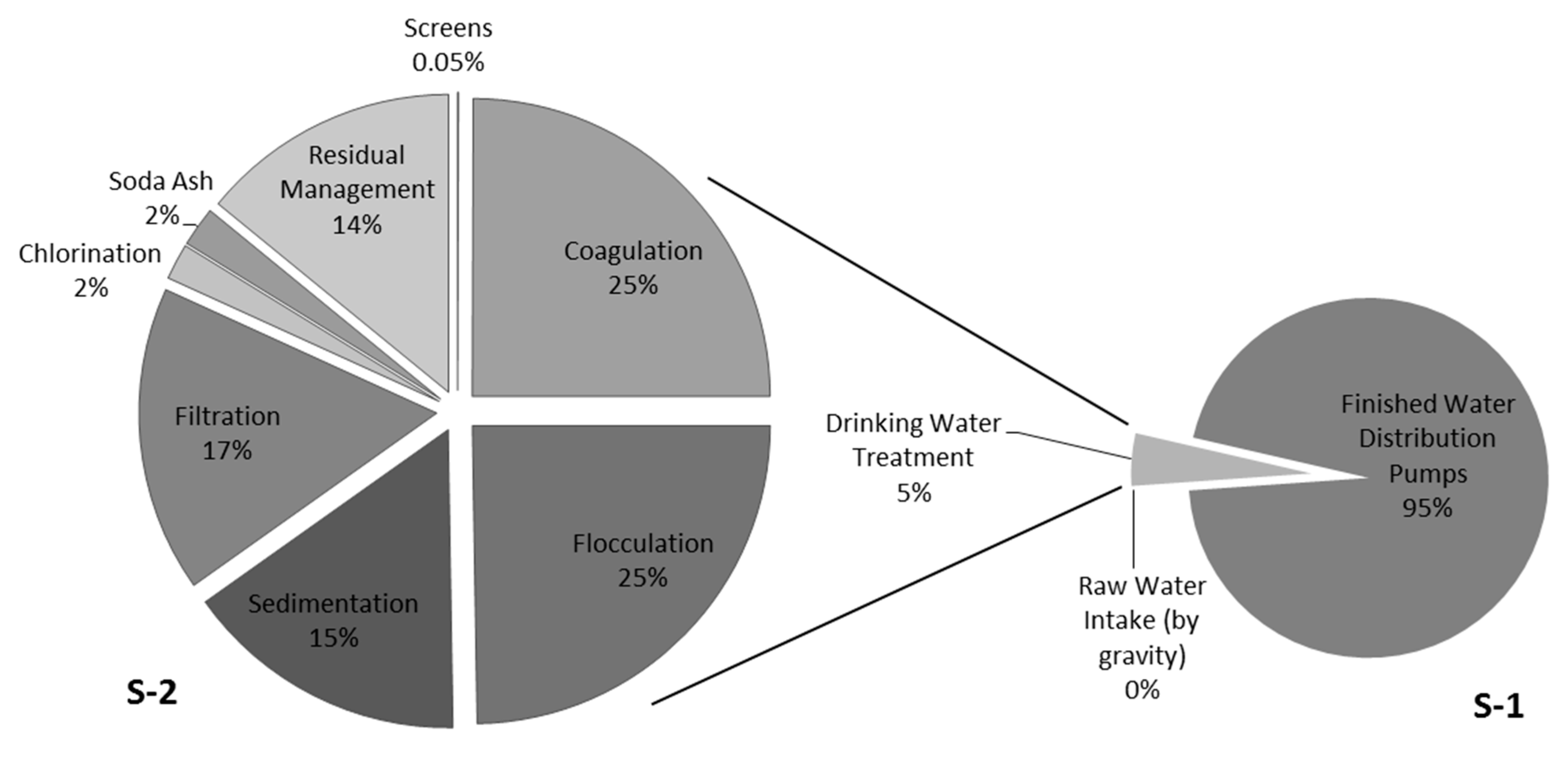
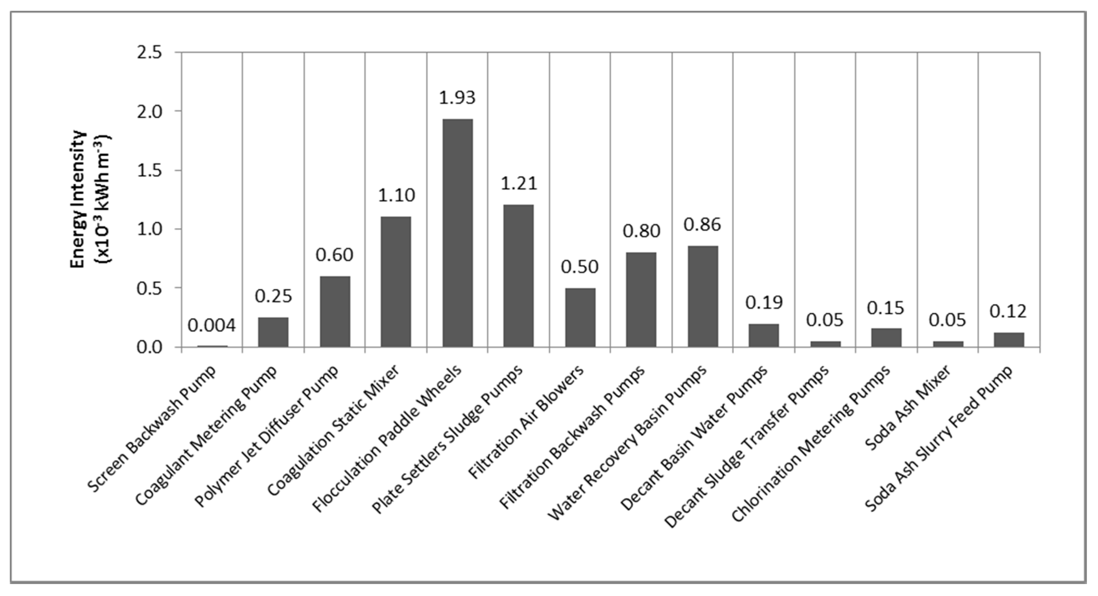
5.1.8. Energy Consumption of the DWTP

The selected DWTP is unique concerning raw water intake. Raw river water flows by gravity from the river canal into the DWTP; thus, no energy is utilized for water intake. For scenario S-1, the total operational energy consumption was 56.3 MWh day⁻¹ (165.3 Wh m⁻³) for the DWTP including water distribution pumps, whereas energy consumption for scenario S-2, i.e., for the DWTP excluding water distribution pumps was 2661 kWh day⁻¹ (7.8 Wh m⁻³). The energy consumption estimated by the current study (Table 5 and

Table 6. Results for estimation of energy consumption for the energy driving units of finished water pumping.

	Energy Driving Units	Plant Motor Size (Data Obtained from Plant’s Managers) (hp)	Estimated Motor Size (This Study) (hp)	Motor Size (This Study) (MWh day−1)	Wire-to-Water Efficiency (%)
Finished Water Pumping	Zone-1 Pump	500	496.5	8.9	80
	Zone-2 Pump	400	404.7	7.2	70
		400	404.7	7.2	70
	Zone-3 Pump	250	248.1	4.4	80
		460	421.1	7.8	80
		500	509.6	9.1	80
		500	509.6	9.1	80
				Total 53.9

, Figure 2 and Figure 3) was validated by comparing the estimated motor sizes to the plant motor sizes. As shown by Table 5 and Table 6, the values are in good agreement with each other.

Water distribution pumps were the largest consumers of electricity, utilizing about 95% of the total operational energy consumption (158.2 Wh m⁻³), while the remaining 5% was utilized for the operation of the DWTP (S-1). Overall, for scenario S-2, it was shown that coagulation and flocculation processes were the largest consumers of energy, consuming about 664 kWh day⁻¹ (1.95 Wh m⁻³) and 659 kWh day⁻¹ (1.93 Wh m⁻³), respectively (Figure 3, Table 5). Pumping operations within the DWTP and the mixing operations (during coagulation, flocculation, and soda ash slurry mixing) utilized about 54% and 40% of the total operational energy consumption of the DWTP, respectively (S-2). Backwashing jet pumps for screens were the smallest consumers of energy within the DWTP, consuming about 0.004 Wh m⁻³ (Figure 3).

Further, unit process-based quantitative assessment of energy intensities as computed in this study may help to compare and improve the performance of treatment plants. Plants of similar capacities may not be utilizing similar paths of treatment. Hence, the energy consumption may be recomputed based on the unit processes being utilized by the plants, resulting in a fairer energy performance comparison (Figure 3). The unit process-based quantitative assessment of energy intensities may help compare the performance of different plants more accurately and may identify opportunities for improvement.

Sensitivity analysis was performed for the energy consumption estimates related to the pumping operation for the treatment plant. Wire-to-electric efficiencies of the pumps were increased by 5% and 10%, which resulted in a 2.6% (2.59 MWh day⁻¹) and 4.9% (2.53 MWh day⁻¹) decrease in the total operational energy consumption (2.66 MWh day⁻¹) of the water treatment units, respectively, whereas decreasing wire-to-water efficiencies by 5% (2.74 MWh day⁻¹) and 10% (2.82 MWh day⁻¹) resulted in increased total operational energy consumption by 2.8% and 6%.

Various studies have been conducted to evaluate the energy consumption of treatment plants. Ref. [62] determined energy consumption for a large-scale water treatment plant in the Netherlands and reported a total energy consumption of 172 Wh m⁻³ for the treatment plant, including intake pumps and water distribution pumps. Ref. [105] reported that in the U.S. the average electricity use for water supply systems, including water pumping, treatment, and distribution, amounted to about 369.8 Wh m⁻³, whereas that of New York State was about 186.2 Wh m⁻³.

The methodology developed in this work is applicable to estimating energy consumption for plants treating either surface or groundwater sources. Because the energy computations are based on unit operations, one can simply lay out the units in any desirable configuration. For example, for a groundwater source, typically only filtration and disinfection units would be needed. In this study, the computation does not involve advanced treatment units such as ozonation, membrane filtration, or UV disinfection. This is because these units were not part of the example DWTP, which uses conventional treatment and does not employ/require these advanced techniques for the treatment of their raw water. However, energy considerations of advanced treatment units have been recently published in other studies [106].

Usually, water treatment plants do not have energy consumption instrumentation installed in individual unit processes; rather, they have totalizers for large sessions of the plant. The reason is the high cost associated with instrumentation. Indeed, for this reason most water or wastewater treatment plants do not have this information and cannot benchmark their energy consumption when contemplating switching to renewable sources of energy. In sustainability studies, and in consideration of energy savings, many plants have struggled with lack of data. Even in southwestern U.S., where the plants are relatively new and modern, such data do not exist. The methodology proposed in this study, to overcome the lack of energy consumption data in treatment plants, considers every individual unit of operation present in a treatment plant, and thus equipment-level energy consumption was computed. In addition, the method developed uses motors (considering their respective efficiencies) as the major energy-consuming unit. The design equations proposed, based on typical engineering design parameters and equipment manufacturer data, can be used by any plant to estimate their energy consumption, independent of the existence of electricity consumption meters installed in their unit operations. The need to establish acceptable approaches to compute energy consumption in treatment plants was also recently evidenced by [107].

The plant uses a conventional treatment train (utilizing the processes of coagulation, flocculation, sedimentation, filtration, and disinfection) for water treatment. Other typical treatment trains employed for drinking water treatment are direct filtration (utilizing the processes of coagulation, flocculation, filtration, and disinfection) and inline filtration (utilizing the processes of coagulation, filtration, and disinfection). Thus, the current work covers all the basic treatment processes used by a typical DWTP for water treatment. The design criteria followed by this study are based on industry-accepted design criteria and can be applied with some modifications for any treatment plant. This work is unique because it provides information about the detailed design and the energy consumption evaluation, along with references for replication of this work. Further, the provided information is valuable and meaningful and can help design engineers and researchers alike for application of this work to their treatment plant. The energy consumption evaluation and the potential for solar energy application on plants of various sizes and complexity using the same methodology have been determined by other studies [6,7]. Ref. [6] determined the energy consumption of a plant, which treats 0.425 m³ of groundwater per second by utilizing the processes of coagulation, filtration, and disinfection (inline filtration). Ref. [7] determined the energy consumption of a treatment plant that treats 1 Mm³ of raw river water per day by using direct filtration process. Thus, the methodology developed in this work can be applied for design and energy consumption evaluation of other treatment plants.

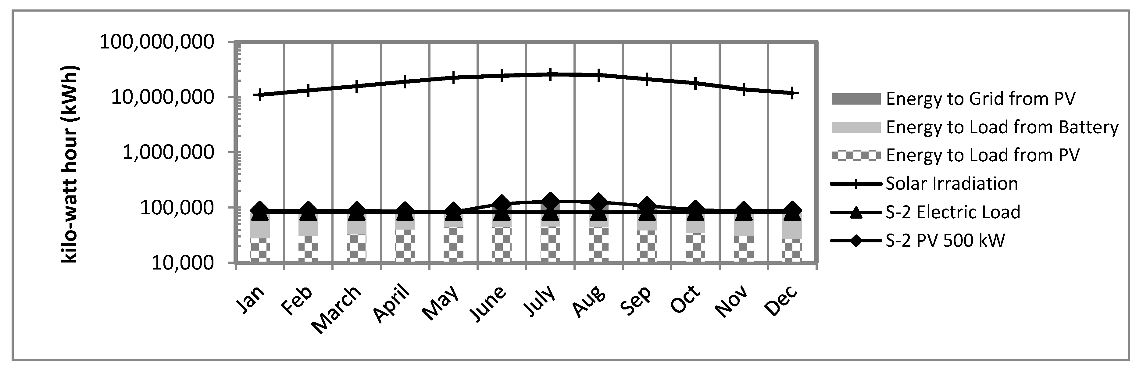
5.2. System Advisor Model

Results achieved using SAM for the PV design and economic analysis are summarized as follows. The techno-economic evaluation was only conducted for scenario S-2, i.e., to offset the energy consumption of the DWTP excluding distribution pumps. A 500 kW PV system was sized, with large storage capacity incurring a net capital cost of $14.5M (

Table 7. Results for technical and financial analysis of solar PV system using the system advisor model for scenario S-2 (analysis for energy consumption of water treatment plant excluding distribution pumps) for locations of Nevada and New York.

	Parameter	Unit	Nevada Location	New York Location
Module	Nameplate Capacity	kW	500	850
	Number of Modules	-	1630	2780
	Modules per String	-	10	10
	Strings in Parallel	-	163	278
	Total Module Area	×103 m2	3.18	5.43
	String Voc	Volt	451	451
	String Vmp	Volt	366.5	366.5
Inverter	Total Capacity	kWac	410	709.6
	Number of Inverters	-	41	71
	Maximum DC Voltage	Volt	600	600
	Minimum MPPT Voltage	Volt	300	300
	Maximum MPPT Voltage	Volt	500	500
	DC to AC Ratio	-	1.2	1.2
	Total Land Area	×103 m2	10.5	18.2
Battery	Nominal Bank Capacity	MWh	75.1	82.2
	Nominal Bank Voltage	Volt	350	350
	Cell in Series	-	175	175
	Strings in Parallel	-	167	183
	Battery Efficiency	%	92.7	92.7
Financial	Net Present Value	$ million	0.24	−0.68
Metrics	Levelized cost of Electricity (nominal)	Cents kWh−1	2.65	9.68
	Levelized cost of Electricity (real)	Cents kWh−1	2.15	7.84
	Net Capital Cost	$ million	14.5	16.5
	Electricity Bill without System (year 1)	$ million	0.08	0.07
	Electricity Bill with System (year 1)	$	6444	0

). Monthly performance of the PV system is shown in Figure 4. There is a yearly electricity bill of $6444 (Table 7); since the system is grid-connected, these are the fixed yearly costs for grid connection.

5.2.1. Effect of Battery Storage

The DWTP operates 24 h a day, hence, to meet the nighttime energy requirements, as well to ensure a balanced supply of energy, battery storage was provided. The battery type chosen was lead acid flooded. Results showed that the battery storage comprised over 80% of the capital costs of the PV system (Table 7). Even though the NPV was positive, the value is small compared to the net capital costs incurred. A higher NPV is better than a lower NPV. A scenario was simulated by decreasing the battery prices from $157.7 kWh⁻¹ to $15.77 kWh⁻¹. This resulted in net capital costs of $3M and a positive NPV for the PV system. The results show that for solar energy to become an attractive prospect for investors, and a reliable source of electricity throughout the 24 h, prices for battery storage must decrease substantially. The DWTP was also analyzed without incorporating battery storage (assuming all other parameters remain the same), for comparison purposes and to reflect the effect of battery storage on cost and performance of the PV system. In this case, the PV system would rely on grid connection to meet the nighttime energy requirements for the plant. It was determined that a PV system without storage has the potential to offset 2.2% (500 kW system, net capital costs $1.7 M, NPV $0.16 M) of the electric load, respectively.

It can be seen that the cost incurred when battery storage was not incorporated was much lower, compared to when storage was provided. The cost associated with battery storage, comprised over 80% of the PV system costs. Successful cost recovery of the PV system with battery storage during the lifetime of the PV would require application of novel approaches for the production of low-cost battery storage systems [108], which would greatly promote the role of solar PV systems as a viable and competitive source of electricity generation for the 24-h duration of the day.

Various studies have explored the use of renewables for water treatment. Ref. [61] compared the performance of a conventional DWTP and a wind-solar-powered nano-filtration pilot plant located in Spain. The study concluded that the application of a nano-filtration process resulted in higher quality water, and usage of renewables not only assisted in making an energy-intensive process sustainable but also helped in making the water treatment process more efficient. Ref. [62] explored the potential of using wind and solar energy for a water treatment plant located in the Netherlands. The study found that about 70–96% of energy independence can be achieved by using 8 MW wind turbines and 5.6 MW solar panels, but due to high costs for large battery storage, 100% energy independence could not be achieved. Solar energy was used in conjunction with wind energy because the site possessed large but erratic wind potential while solar energy using photovoltaics provided a more balanced supply. Ref. [109] determined solar PV to be viable for meeting the electricity needs of two villages located in Bangladesh.

5.2.2. Effect of Governmental Incentives

Financial analysis heavily relies on governmental incentives. Two incentives were applied, federal investment tax incentive and the state property tax exemption incentive for this study for the Nevada site, resulting in a nominal LOCE of 2.65 cents kWh⁻¹. If either of these incentives were removed from the analysis, the development of solar PV would no longer be profitable as it would result in a negative NPV and increased LCOE. Ref. [82] reported LCOE values for commercial PV systems in the U.S. in the range of 9–12 cents kWh⁻¹ when not incorporating federal ITC and in the range of 6‒8 cents kWh⁻¹ when incorporating it. For the current study, when the 30% ITC was not incorporated, the NPV became negative while the nominal LCOE value was estimated as $0.39 kWh⁻¹.

Based on the renewable portfolio standard (RPS) for the state, 25% of electricity generation by the year 2025 must be achieved using renewables [49]. Portfolio energy credits earned due to the deployment of solar PVs at treatment plants can assist in meeting RPS goals. Incorporating renewables into the existing water infrastructure assists in reducing the dependency of water facilities on the traditional energy sources, thus generating reduced emissions. This helps in making water facilities energy independent, which may lead to cost savings in the long run. Policy makers for water and energy need to participate in collaborative planning and implement policies that provide incentives to existing and future DWTPs for using renewables to offset their energy requirements.

5.2.3. Effect of Location Change

A hypothetical scenario was examined by changing the location of the treatment plant from southwest Nevada (6.3 kWh m⁻² day⁻¹) to the U.S. east coast. The location selected was New York (3.5 kWh m⁻² day⁻¹). The financial parameters used are shown in Table 4. The electric rate input, downloaded from the SAM database for electric rates, was based upon the rates of the New York Power Authority for large general service. The results showed that the PV system (500 kW PV, 75 MWh battery) in the Nevada location (Table 7) when located in New York was able to offset 85% of the total load (2661 MWh day⁻¹) analyzed. Forty-seven percent of the load offset was achieved using battery storage. It was further determined that a 850 kW PV system using a battery storage capacity of 82 MWh was able to offset 100% of the 2661 MWh day⁻¹ electric load, for the New York location, however, the NPV was negative (Table 7). Fifty-eight percent of the load offset was achieved using battery storage.

5.2.4. Sensitivity Analysis

Sensitivity analysis for the financial parameters that were changed when analyzing for the Nevada and New York locations showed that property tax rates had the largest effect. For the New York location, the NPV changed from negative to positive, when the property tax rate was changed from 2% to 1.2%, respectively. The property tax rate may vary depending upon the location of the property. A property tax exemption or partial property rate incentives have the potential of greatly promoting the development of solar facilities in the state.

Sensitivity analysis was also performed for various financial parameters for the solar system sited in Nevada and showed that a discount rate of 7% or less resulted in a negative NPV. For the current study, a debt percentage of 100% was used. A debt percentage of 96% or less rendered a negative NPV and higher LCOE. Reducing the loan term decreases the NPV and increases the LCOE. Using a loan term of 23 years or less, or loan interest rates of 4% or higher, resulted in a negative NPV. For the current study, an inflation rate of 2.5% was used. Using an inflation rate of 1.9% or less resulted in a negative NPV. It can be seen that for this particular study, the viability of the project is sensitive to the changes in discount rate, inflation rate, debt percentage, loan interest rates, and loan term. For the same PV system, if battery storage is not provided, a debt % of 85% or less, loan term of 18 years or less, discount rate of 4% or less, interest rate of 6% or higher, and inflation rate of zero or less rendered a negative NPV and higher LCOE values.

Ref. [46] determined the economic feasibility of using solar PVs to fulfill the electricity needs of a rural community consisting of 300 homes, located in Gusau, Nigeria. The study found that solar PVs was highly sensitive to changes in electricity rates and inflation rates but slightly sensitive to changes in loan term and loan interest rate. Changes in year-round insolation levels due to change in location may also significantly alter the energy output of PV systems and thus the results of financial analysis as well [46,110]. Ref. [110] conducted a techno-economic assessment of using solar and wind energy with storage systems for locations in the Kingdom of Saudi Arabia (KSA), Canada, and Australia. The study determined the cost of electricity to be lowest for the Yanbu area in KSA (0.609 $ kWh⁻¹). Further, the study determined the renewable potential of the KSA to be better than the selected locations in Canada and Australia due to higher year-round levels of solar irradiance.

5.3. Land Area Requirements

The land coverage of the PV system for the DWTP (S-2) was 0.01 km² (Table 7). The empty real estate acreage of the DWTP was about 0.4 km², estimated using ArcGIS. Hence, it can be seen that ample land area was available for development of solar PV, and additional costs need not be incurred for the purpose of purchasing land for solar development. Moreover, ample empty land area is available near the DWTP that can be acquired for the installation of PV.

Various studies have analyzed the land area demands of solar installations. Ref. [111] determined that about 15% of the total land area of Iran provided excellent conditions for solar installations. Ref. [112] determined optimal sites in Afghanistan for the development of wind and solar energy systems, resulting in potential generations of 0.34 million GWh per year and 0.15 million GWh per year, respectively.

5.4. Carbon Emissions

Net reduction in carbon emissions was found to be 450 metric tons CO₂-eq year⁻¹ (equivalent to one year emissions for: 95 passenger cars driven, electricity consumption of 67 homes, or carbon sequestration due to 530 acres of U.S. forests). Without battery storage, the net reduction in carbon emissions was found to be 240 metric tons CO₂-eq year⁻¹ (equivalent to one year emissions for: 50 passenger cars driven, electricity consumption of 35 homes, or carbon sequestration due to 280 acres of U.S. forests). The equivalencies were calculated using the USEPA GHG Equivalencies Calculator [113].

Ref. [114] calculated the reduction in carbon emissions due to residential installations of solar PV in Australia and determined it to be 3.7 million ton CO₂-eq in the year 2013 and 8 million ton CO₂-eq in the year 2020. Ref. [115] estimated a GHG reduction of 1.7 ton year⁻¹ for a zero energy solar home in São Paulo, Brazil. Ref. [116] developed a simulation model incorporating estimated future costs for renewables of wind and solar and determined an 80% reduction in carbon emissions by the year 2030 relative to the levels of the year 1990, without any rise in LCOE.

In general, this study evaluated the energy consumption and integration of renewable energy sources into existing water treatment plants for energy sufficiency purposes. Further, the gains achieved in public health and environmental impacts due to reduction in carbon emissions makes the development of solar PVs a good investment [117].

6. Conclusions

The objective of this study was to utilize solar PVs to meet the energy demands of an existing DWTP treating 3.94 m³ of river water per second by (a) designing and determining the energy consumption of each unit operation of the treatment plant, (b) sizing the DWTP for solar PVs based on available land holdings and economic analysis, and (c) determining the net reduction in carbon emissions due to the development of solar PVs. The analysis was successfully conducted for scenario S-1 (100% of electric load) and scenario S-2 (5% of electric load, i.e., excluding water distribution pumps), with battery storage and without storage.

For scenario S-1, total operational energy consumption was 56.3 MWh day⁻¹ (165.3 Wh m⁻³) for the DWTP including water distribution pumps, whereas energy consumption for S-2, i.e., for the DWTP excluding water distribution pumps, was 2661 kWh day⁻¹ (7.8 Wh m⁻³). For S-1, water distribution pumps utilized 95% of the total operational energy consumption, whereas the water treatment only operations (S-2) utilized the remaining 5% of the total operational energy consumption of the DWTP. Energy intensity values were determined for the processes of coagulation (1.95 Wh m⁻³), flocculation (1.93 Wh m⁻³), sedimentation (1.2 Wh m⁻³), filtration (1.3 Wh m⁻³), chlorination (0.15 Wh m⁻³), residual management (1.1 Wh m⁻³), and a soda ash system (0.17 Wh m⁻³).

Based on the results of the quantitative analysis of energy consumption, a techno-economic assessment was conducted for solar PVs, to offset the energy consumption of the plant for scenario S-2 only. The development of a 500 kW PV system with battery storage of 75 MWh was found to have a positive net present value of $0.24M, only after the federal and state incentives were incorporated in the analysis. Further, the study showed that reduction in battery prices can tremendously help solar PVs to become a viable source of electricity generation for the entire 24-h duration of the day. Economic feasibility was dependent upon the selection of financial parameters, based on the review of existing literature published between the years 2016 and 2017. Changes in the values of these parameters can greatly affect the results of cost analysis. The economics of solar PVs was found to be sensitive to changes in debt %, inflation rate, loan term, loan interest rates, and discount rates. The real estate acreage of the DWTP was found to be sufficient for the development of solar PVs, which was found to utilize a land area of 0.01 km². The net reduction in carbon emissions because of a solar-based design, with and without the provision of battery storage, was found to be 450 and 240 metric tons CO₂-eq year⁻¹, respectively. It was also determined that changing the plant’s location from the southwest (higher insolation levels) to the east coast (lower insolation levels) would require a larger PV system size and battery storage capacity and thus increased costs. These results were found to be most sensitive to property tax rate, among the parameters changed between the two locations (sales tax, state income tax, property tax, electric rates). Property tax exemption or partial property tax rate incentives were shown to have promising implications for solar development.

In this study, determination of energy consumption was limited to drinking water treatment operation. Future work may include evaluation of energy consumption related to drinking water distribution within the community.

The design approach utilized for the plant, and equations used, highlighted important design factors that may be adjusted to reduce the energy needs of the plants. Energy intensity values generated rigorously for various processes for the plant may allow a more accurate comparison of a plant’s performance against that of other plants. This method can be used for other plants by making suitable alterations. Studies like these can provide the right motivation for increasing the efforts towards a low-carbon water sector or carbon-neutral water infrastructure. Further, the detailed aspects of the design of actual plants are generally not shared publically, and thus this work provides valuable insight for engineering professionals and decision makers. This methodology can be applied to other DWTPs with some alterations for attainment of sustainability goals. The deployment of solar PVs will help achieve the effects of increased public and environmental health and climate benefits.

References

1. Dow, C.; Ahmad, S.; Stave, K.; Gerrity, D. Evaluating the Sustainability of IPR and DPR: A Southern Nevada Case Study. AWWA Water Sci. 2019, 1, e1153. [Google Scholar] [CrossRef] [PubMed] [Green Version]
2. U.S. Environmental Protection Agency (USEPA). 2019. Available online: https://www.epa.gov/sustainable-water-infrastructure/energy-efficiency-water-utilities (accessed on 25 December 2019).
3. Shrestha, E.; Ahmad, S.; Johnson, W.; Batista, J.R. The carbon footprint of water management policy options. Energy Policy 2012, 42, 201–212. [Google Scholar] [CrossRef]
4. Shrestha, E.; Ahmad, S.; Johnson, W.; Shrestha, P.; Batista, J.R. Carbon footprint of water conveyance versus desalination as alternatives to expand water supply. Desalination 2011, 280, 33–43. [Google Scholar] [CrossRef]
5. Goldstein, R.; Smith, W. Water & Sustainability (Volume 4): US Electricity Consumption for Water Supply & Treatment-the Next Half Century; Electric Power Research Institute: Palo Alto, CA, USA, 2002. [Google Scholar]
6. Bukhary, S.; Batista, J.; Ahmad, S. An Analysis of Energy Consumption and the Use of Renewables for a Small Drinking Water Treatment Plant. Water 2020, 12, 28. [Google Scholar] [CrossRef] [Green Version]
7. Bukhary, S.; Batista, J.; Ahmad, S. Water-Energy-Carbon Nexus Approach for Sustainable Large-Scale Drinking Water Treatment Operation. J. Hydrol. 2020, 587, 124953. [Google Scholar] [CrossRef]
8. Bukhary, S.; Weidhaas, J.; Ansari, K.; Mahar, R.B.; Pomeroy, C.; Van Derslice, J.A.; Burian, S.; Ahmad, S. Using Distributed Solar for Treatment of Drinking Water in Developing Countries. In Proceedings of the World Environmental and Water Resources Congress 2017, Sacramento, CA, USA, 21–25 May 2017; Volume 2017, pp. 264–276. [Google Scholar] [CrossRef]
9. Plappally, A.K.; Lienhard, V.J.H. Energy requirements for water production, treatment, end use, reclamation, and disposal. Renew. Sustain. Energy Rev. 2012, 16, 4818–4848. [Google Scholar] [CrossRef]
10. Sala-Garrido, R.; Molinos-Senante, M. Benchmarking energy efficiency of water treatment plants: Effects of data variability. Sci. Total Environ. 2020, 701, 134960. [Google Scholar] [CrossRef]
11. Vadasarukkai, Y.S.; Gagnon, G.A. Influence of the Mixing Energy Consumption Affecting Coagulation and Floc Aggregation. Environ. Sci. Technol. 2017, 51, 3480–3489. [Google Scholar] [CrossRef] [Green Version]
12. Wakeel, M.; Chen, B.; Hayat, T.; Alsaedi, A.; Ahmad, B. Energy consumption for water use cycles in different countries: A review. Appl. Energy 2016, 178, 868–885. [Google Scholar] [CrossRef]
13. Awad, H.; Alalm, M.G.; El-Etriby, H.K. Environmental and cost life cycle assessment of different alternatives for improvement of wastewater treatment plants in developing countries. Sci. Total Environ. 2019, 660, 57–68. [Google Scholar] [CrossRef]
14. Chang, J.; Lee, W.; Yoon, S. Energy consumptions and associated greenhouse gas emissions in operation phases of urban water reuse systems in Korea. J. Clean. Prod. 2017, 141, 728–736. [Google Scholar] [CrossRef]
15. Gude, V.G. Energy and water autarky of wastewater treatment and power generation systems. Renew. Sustain. Energy Rev. 2015, 45, 52–68. [Google Scholar] [CrossRef]
16. He, Y.; Zhu, Y.; Chen, J.; Huang, M.; Wang, P.; Wang, G.; Zou, W.; Zhou, G. Assessment of energy consumption of municipal wastewater treatment plants in China. J. Clean. Prod. 2019, 228, 399–404. [Google Scholar] [CrossRef]
17. Mannina, G.; Rebouças, T.F.; Cosenza, A.; Chandran, K. A plant-wide wastewater treatment plant model for carbon and energy footprint: Model application and scenario analysis. J. Clean. Prod. 2019, 217, 244–256. [Google Scholar] [CrossRef]
18. Dawadi, S.; Ahmad, S. Changing climatic conditions in the Colorado River Basin: Implications for water resources management. J. Hydrol. 2012, 430, 127–141. [Google Scholar] [CrossRef]
19. Dawadi, S.; Ahmad, S. Evaluating the impact of demand-side management on water resources under changing climatic conditions and increasing population. J. Environ. Manag. 2013, 114, 261–275. [Google Scholar] [CrossRef]
20. Ahmad, S.; Prashar, D. Evaluating Municipal Water Conservation Policies Using a Dynamic Simulation Model. Water Resour. Manag. 2010, 24, 3371–3395. [Google Scholar] [CrossRef]
21. Qaiser, K.; Ahmad, S.; Johnson, W.; Batista, J. Evaluating the impact of water conservation on fate of outdoor water use: A study in an arid region. J. Environ. Manag. 2011, 92, 2061–2068. [Google Scholar] [CrossRef]
22. Qaiser, K.; Ahmad, S.; Johnson, W.; Batista, J.R. Evaluating water conservation and reuse policies using a dynamic water balance model. Environ. Manag. 2013, 51, 449–458. [Google Scholar] [CrossRef]
23. U.S. Environmental Protection Agency (USEPA). 2016. Available online: https://www3.epa.gov/region9/waterinfrastructure/ (accessed on 15 September 2016).
24. Xue, X.; Hawkins, T.R.; Schoen, M.E.; Garland, J.; Ashbolt, N.J. Comparing the life cycle energy consumption, global warming and eutrophication potentials of several water and waste service options. Water 2016, 8, 154. [Google Scholar] [CrossRef] [Green Version]
25. Bukhary, S.; Chen, C.; Kalra, A.; Ahmad, S. Improving Streamflow Reconstructions Using Oceanic-Atmospheric Climate Variability. In Proceedings of the World Environmental and Water Resources Congress 2014, Portland, Oregon, 1–5 June 2014; pp. 846–855. [Google Scholar] [CrossRef]
26. Bukhary, S.; Kalra, A.; Ahmad, S. Insights into reconstructing sacramento river flow using tree rings and Pacific Ocean climate variability. In Proceedings of the World Environmental and Water Resources Congress, Austin, TX, USA, 17–21 May 2015; pp. 1040–1049. [Google Scholar] [CrossRef]
27. Choubin, B.; Khalighi-Sigaroodi, S.; Malekian, A.; Ahmad, S.; Attarod, P. Drought forecasting in a semi-arid watershed using climate signals: A neuro-fuzzy modeling approach. J. Mt. Sci. 2014, 11, 1593–1605. [Google Scholar] [CrossRef]
28. Nussbaum, E.M.; Owens, M.C.; Sinatra, G.M.; Rehmat, A.P.; Cordova, J.R.; Ahmad, S.; Dascalu, S.M. Losing the Lake: Simulations to Promote Gains in Student Knowledge and Interest about Climate Change. Int. J. Environ. Sci. Educ. 2015, 10, 789–811. [Google Scholar]
29. Chen, C.; Kalra, A.; Ahmad, S. Hydrologic responses to climate change using downscaled GCM data on a watershed scale. J. Water Clim. Chang. 2019, 10, 63–77. [Google Scholar] [CrossRef]
30. Tamaddun, K.A.; Kalra, A.; Ahmad, S. Spatiotemporal Variation in the Continental US Streamflow in Association with Large-Scale Climate Signals Across Multiple Spectral Bands. Water Resour. Manag. 2019, 33, 1947–1968. [Google Scholar] [CrossRef]
31. Tamaddun, K.; Kalra, A.; Kumar, S.; Ahmad, S. CMIP5 Models’ Ability to Capture Observed Trends under the Influence of Shifts and Persistence: An In-depth Study on the Colorado River Basin. J. Appl. Meteorol. Climatol. 2019, 58, 1677–1688. [Google Scholar] [CrossRef]
32. Nazari-Sharabian, M.; Ahmad, S.; Karakouzian, M. Climate Change and Eutrophication: A Short Review. Eng. Technol. Appl. Sci. Res. 2018, 8, 3668–3672. [Google Scholar]
33. Nazari-Sharabian, M.; Taheriyoun, M.; Ahmad, S.; Karakouzian, M.; Ahmadi, A. Water Quality Modeling of Mahabad Dam Watershed–Reservoir System under Climate Change Conditions, Using SWAT and System Dynamics. Water 2019, 11, 394. [Google Scholar] [CrossRef] [Green Version]
34. Thakur, B.; Kalra, A.; Ahmad, S.; Lamb, K.; Lakshmi, V. Bringing Statistical Learning Machines together for Hydro-climatological Predictions—Case Study for Sacramento San Joaquin River Basin, California. J. Hydrol. Reg. Stud. 2020, 27, 100651. [Google Scholar] [CrossRef]
35. Nyaupane, N.; Thakur, B.; Kalra, A.; Ahmad, S. Evaluating Future Flood Scenarios Using CMIP5 Climate Projections. Water 2018, 10, 1866. [Google Scholar] [CrossRef] [Green Version]
36. Saifullah, M.; Liu, S.; Tahir, A.A.; Zaman, M.; Ahmad, S.; Adnan, M.; Chen, D.; Ashraf, M.; Mehmood, A. Development of Threshold Levels and a Climate-Sensitivity Model of the Hydrological Regime of the High-Altitude Catchment of the Western Himalayas, Pakistan. Water 2019, 11, 1454. [Google Scholar] [CrossRef] [Green Version]
37. Rahaman, M.M.; Thakur, B.; Kalra, A.; Ahmad, S. Modeling of GRACE-Derived Groundwater Information in the Colorado River Basin. Hydrology 2019, 6, 19. [Google Scholar] [CrossRef] [Green Version]
38. Yang, T.; Li, Q.; Ahmad, S.; Zhou, H.; Li, L. Changes in Snow Phenology from 1979 to 2016 over the Tianshan Mountains, Central Asia. Remote Sens. 2019, 11, 499. [Google Scholar] [CrossRef] [Green Version]
39. Tamaddun, K.A.; Kalra, A.; Bernardez, M.; Ahmad, S. Effects of ENSO on Temperature, Precipitation, and Potential Evapotranspiration of North India’s Monsoon: An Analysis of Trend and Entropy. Water 2019, 11, 189. [Google Scholar] [CrossRef] [Green Version]
40. Amoueyan, E.; Ahmad, S.; Eisenberg, J.; Gerrity, D. A Dynamic Quantitative Microbial Risk Assessment for Norovirus in Potable Reuse Systems. Microb. Risk Anal. 2020, 14, 100088. [Google Scholar] [CrossRef]
41. Amoueyan, E.; Ahmad, S.; Eisenberg, J.N.S.; Gerrity, D. Equivalency of Indirect and Direct Potable Reuse Paradigms based on a Quantitative Microbial Risk Assessment Framework. Microb. Risk Anal. 2019, 12, 60–75. [Google Scholar] [CrossRef]
42. Amoueyan, E.; Ahmad, S.; Eisenberg, J.N.S.; Pecson, B.; Gerrity, D. Quantifying pathogen risks associated with potable reuse: A risk assessment case study for Cryptosporidium. Water Res. 2017, 119, 255–266. [Google Scholar] [CrossRef]
43. Crittenden, J.C.; Trussell, R.R.; Hand, D.W.; Howe, K.J.; Tchobanoglous, G. MWH’s Water Treatment: Principles and Design; John Wiley & Sons: Hoboken, NJ, USA, 2012. [Google Scholar]
44. Bukhary, S.; Batista, J.; Ahmad, S. Evaluating the Feasibility of Photovoltaic-Based Plant for Potable Water Treatment. In Proceedings of the World Environmental and Water Resources Congress, Sacramento, CA, USA, 21–25 May 2017; pp. 256–263. [Google Scholar] [CrossRef]
45. Bukhary, S.; Ahmad, S.; Batista, J. Analyzing land and water requirements for solar deployment in the Southwestern United States. Renew. Sustain. Energy Rev. 2018, 82, 3288–3305. [Google Scholar] [CrossRef]
46. Okoye, C.O.; Oranekwu-Okoye, B.C. Economic feasibility of solar PV system for rural electrification in Sub-Sahara Africa. Renew. Sustain. Energy Rev. 2018, 82, 2537–2547. [Google Scholar] [CrossRef]
47. Ferreira, A.; Kunh, S.S.; Fagnani, K.C.; De Souza, T.A.; Tonezer, C.; Dos Santos, G.R.; Coimbra-Araújo, C.H. Economic overview of the use and production of photovoltaic solar energy in brazil. Renew. Sustain. Energy Rev. 2018, 81, 181–191. [Google Scholar] [CrossRef]
48. Linssen, J.; Stenzel, P.; Fleer, J. Techno-economic analysis of photovoltaic battery systems and the influence of different consumer load profiles. Appl. Energy 2017, 185, 2019–2025. [Google Scholar] [CrossRef]
49. DSIRE. Database of State Incentives for Renewables & Efficiency (DSIRE). 2017. Available online: http://www.dsireusa.org/ (accessed on 16 August 2017).
50. Brown, K.E.; Henze, D.K.; Milford, J.B. How accounting for climate and health impacts of emissions could change the US energy system. Energy Policy 2017, 102, 396–405. [Google Scholar] [CrossRef]
51. Prehoda, E.W.; Pearce, J.M. Potential lives saved by replacing coal with solar photovoltaic electricity production in the US. Renew. Sustain. Energy Rev. 2017, 80, 710–715. [Google Scholar] [CrossRef] [Green Version]
52. Nonhebel, S. Renewable energy and food supply: Will there be enough land? Renew. Sustain. Energy Rev. 2005, 9, 191–201. [Google Scholar] [CrossRef]
53. Bukhary, S.; Batista, J.; Ahmad, S. Using Solar and Wind Energy for Water Treatment in the Southwest. In Proceedings of the World Environmental and Water Resources Congress, Pittsburgh, PA, USA, 19–23 May 2019; Volume 2019, pp. 410–416. [Google Scholar] [CrossRef]
54. Bukhary, S.; Batista, J.; Ahmad, S. Sustainable Desalination of Brackish Groundwater for the Las Vegas Valley. In Proceedings of the World Environmental and Water Resources Congress 2018, Minneapolis, MN, USA, 3–7 June 2018. [Google Scholar] [CrossRef]
55. Gilman, P.; Blair, N.; Mehos, M.; Christensen, C.; Janzou, S.; Cameron, C. Solar Advisor Model User Guide for Version 2.0; National Renewable Energy Laboratory: Golden, CO, USA, 2008.
56. Good, J.; Johnson, J.X. Impact of inverter loading ratio on solar photovoltaic system performance. Appl. Energy 2016, 177, 475–486. [Google Scholar] [CrossRef]
57. Phillips, C.; Elmore, R.; Melius, J.; Gagnon, P.; Margolis, R. A data mining approach to estimating rooftop photovoltaic potential in the US. J. Appl. Stat. 2019, 46, 385–394. [Google Scholar] [CrossRef]
58. Sweeney, J.F.; Pate, M.B.; Choi, W. Life cycle production and costs of a residential solar hot water and grid-connected photovoltaic system in humid subtropical Texas. J. Renew. Sustain. Energy 2016, 8, 053702. [Google Scholar] [CrossRef]
59. Song, J.; Choi, Y. Design of photovoltaic systems to power aerators for natural purification of acid mine drainage. Renew. Energy 2015, 83, 759–766. [Google Scholar] [CrossRef]
60. Bukhary, S. Water-Energy Nexus Approaches for Solar Development and Water Treatment in the Southwestern United States. Ph.D. Thesis, University of Nevada Las Vegas (UNLV), Las Vegas, NV, USA, 2018. [Google Scholar]
61. García-Vaquero, N.; Lee, E.; Castañeda, R.J.; Cho, J.; López-Ramírez, J.A. Comparison of drinking water pollutant removal using a nanofiltration pilot plant powered by renewable energy and a conventional treatment facility. Desalination 2014, 347, 94–102. [Google Scholar] [CrossRef]
62. Soshinskaya, M.; Crijns-Graus, W.H.; van der Meer, J.; Guerrero, J.M. Application of a microgrid with renewables for a water treatment plant. Appl. Energy 2014, 134, 20–34. [Google Scholar] [CrossRef] [Green Version]
63. Astolfi, M.; Mazzola, S.; Silva, P.; Macchi, E. A synergic integration of desalination and solar energy systems in stand-alone microgrids. Desalination 2017, 419, 169–180. [Google Scholar] [CrossRef]
64. Gikas, P.; Tsoutsos, T. Near zero energy wastewater treatment plants for the Greek islands. Desalin. Water Treat. 2015, 53, 3328–3334. [Google Scholar] [CrossRef]
65. Ganiyu, S.O.; Brito, L.R.; de Araújo Costa, E.C.; dos Santos, E.V.; Martínez-Huitle, C.A. Solar photovoltaic-battery system as a green energy for driven electrochemical wastewater treatment technologies: Application to elimination of Brilliant Blue FCF dye solution. J. Environ. Chem. Eng. 2019, 7, 102924. [Google Scholar] [CrossRef]
66. Nawarkar, C.J.; Salkar, V.D. Solar powered electrocoagulation system for municipal wastewater treatment. Fuel 2019, 237, 222–226. [Google Scholar] [CrossRef]
67. Li, S.; Cai, Y.H.; Schäfer, A.I.; Richards, B.S. Renewable energy powered membrane technology: A review of the reliability of photovoltaic-powered membrane system components for brackish water desalination. Appl. Energy 2019, 253, 113524. [Google Scholar] [CrossRef]
68. Mostafaeipour, A.; Qolipour, M.; Rezaei, M.; Babaee-Tirkolaee, E. Investigation of off-grid photovoltaic systems for a reverse osmosis desalination system: A case study. Desalination 2019, 454, 91–103. [Google Scholar] [CrossRef]
69. Shalaby, S.M. Reverse osmosis desalination powered by photovoltaic and solar Rankine cycle power systems: A review. Renew. Sustain. Energy Rev. 2017, 73, 789–797. [Google Scholar] [CrossRef]
70. Shawky, H.A.; Abdel Fatah, A.A.; Abo ElFadl, M.M.; El-Aassar, A.H.M. Design of a small mobile PV-driven RO water desalination plant to be deployed at the northwest coast of Egypt. Desalin. Water Treat. 2015, 55, 3755–3766. [Google Scholar] [CrossRef]
71. Zhang, Y.; Sivakumar, M.; Yang, S.; Enever, K.; Ramezanianpour, M. Application of solar energy in water treatment processes: A review. Desalination 2018, 428, 116–145. [Google Scholar] [CrossRef] [Green Version]
72. U.S. Environmental Protection Agency (USEPA). 2016. Available online: https://www.epa.gov/dwstandardsregulations (accessed on 12 October 2016).
73. WEF (Water Environment Federation). Energy Conservation in Water and Wastewater Facilities; Manual of practice No. 32; WEF Press: Cologny, Switzerland, 2009. [Google Scholar]
74. Reynolds, T.D.; Richards, P.A. Unit Operations and Processes in Environmental Engineering; PWS Publishing Company: Boston, MA, USA, 1996. [Google Scholar]
75. Hendricks, D.W. Water Treatment Unit Processes: Physical and Chemical; CRC Press: Boca Raton, FL, USA, 2016. [Google Scholar]
76. Moomaw, W.; Burgherr, P.; Heath, G.; Lenzen, M.; Nyboer, J.; Verbruggen, A. Annex II: Methodology. In IPCC Special Report on Renewable Energy Sources and Climate Change Mitigation; Edenhofer, O., Pichs-Madruga, R., Sokona, Y., Seyboth, K., Matschoss, P., Kadner, S., Zwickel, T., Eickemeier, P., Hansen, G., Schlomer, S., et al., Eds.; Cambridge University Press: Cambridge, UK; New York, NY, USA, 2011. [Google Scholar]
77. U.S. Energy Information Administration (USEIA). 2016. Available online: http://www.eia.gov/state/seds/ (accessed on 29 July 2016).
78. Freecleansolar. 2017. Available online: https://www.freecleansolar.com/Solar-Panel-305-Watt-Helios-7T2-305-p/7t2-305.htm (accessed on 28 August 2017).
79. Wholesalesolar. 2017. Available online: https://www.wholesalesolar.com/2935110/fronius/inverters/fronius-symo-lite-10.0-3-10kw-3-phase-480-inverter (accessed on 28 August 2017).
80. Wholesalesolar. 2017. Available online: https://www.wholesalesolar.com/9901382/surrette-rolls/batteries/surrette-rolls-s-1660-flooded-battery (accessed on 28 August 2017).
81. Fu, R.; Chung, D.; Lowder, T.; Feldman, D.; Ardani, K.; Margolis, R. US Solar Photovoltaic System Cost Benchmark: Q1 2016; National Renewable Energy Laboratory, US Department of Energy: Golden, CO, USA, 2016; NREL/TP-6A20-66532.
82. Fu, R.; Feldman, D.J.; Margolis, R.M.; Woodhouse, M.A.; Ardani, K.B. US Solar Photovoltaic System Cost Benchmark: Q1 2017; National Renewable Energy Laboratory (NREL): Golden, CO, USA, 2017; No. NREL/TP-6A20-68925.
83. Kang, M.H.; Rohatgi, A. Quantitative analysis of the levelized cost of electricity of commercial scale photovoltaics systems in the US. Sol. Energy Mater. Sol. Cells 2016, 154, 71–77. [Google Scholar] [CrossRef]
84. Krupa, J.; Harvey, D. Renewable electricity finance in the United States: A state-of-the-art review. Energy 2017, 135, 913–929. [Google Scholar] [CrossRef]
85. Lai, C.S.; McCulloch, M.D. Levelized cost of electricity for solar photovoltaic and electrical energy storage. Appl. Energy 2017, 190, 191–203. [Google Scholar] [CrossRef]
86. Mundada, A.S.; Shah, K.K.; Pearce, J.M. Levelized cost of electricity for solar photovoltaic, battery and cogen hybrid systems. Renew. Sustain. Energy Rev. 2016, 57, 692–703. [Google Scholar] [CrossRef] [Green Version]
87. Musi, R.; Grange, B.; Sgouridis, S.; Guedez, R.; Armstrong, P.; Slocum, A.; Calvet, N. Techno-economic analysis of concentrated solar power plants in terms of levelized cost of electricity. In AIP Conference Proceedings; AIP Publishing: Abu Dhabi, UAE, 2017; Volume 1850, p. 160018. [Google Scholar]
88. Reiter, E.; Lowder, T.; Mathur, S.; Mercer, M. Virginia Solar Pathways Project. Economic Study of Utility-Administered Solar Programs: Soft Costs, Community Solar, and Tax Normalization Considerations; NREL (National Renewable Energy Laboratory): Golden, CO, USA, 2016; No. NREL/TP-6A42-65758.
89. Racharla, S.; Rajan, K. Solar tracking system—A review. Int. J. Sustain. Eng. 2017, 10, 72–81. [Google Scholar]
90. NDT Nevada Department of Taxation (NDT). 2017. Available online: https://tax.nv.gov/ (accessed on 20 December 2017).
91. McCabe, J. Salvage Value of Photovoltaic Systems. In Proceedings of the World Renewable Energy Forum, Littleton, CO, USA, 2011; Available online: https://ases.conference-services.net/resources/252/2859/pdf/SOLAR2012_0783_full%20paper.pdf (accessed on 8 June 2017).
92. McKinney, R.E. Environmental Pollution Control Microbiology: A Fifty-Year Perspective; CRC Press: Boca Raton, FL, USA, 2004. [Google Scholar]
93. Lee, C.C.; Lin, S.D. Handbook of Environmental Engineering Calculations; McGraw Hill: New York, NY, USA, 2007. [Google Scholar]
94. Mays, L.W. Water Resources Engineering; John Wiley & Sons: Hoboken, NJ, USA, 2006. [Google Scholar]
95. Kawamura, S. Integrated Design of Water Treatment Facilities; John Willey & Sons: New York, NY, USA, 1991. [Google Scholar]
96. Qasim, S.R. Wastewater Treatment Plants: Planning, Design, and Operation; CRC Press: Boca Raton, FL, USA, 1998. [Google Scholar]
97. Lauer, W.; Barsotti, M.G.; Hardy, D.K. Chemical Feed Field Guide for Treatment Plant Operators; American Water Works Association: Denver, CO, USA, 2009. [Google Scholar]
98. Lawler, D.F.; Singer, P.C. Analyzing disinfection kinetics and reactor design: A conceptual approach versus the SWTR. J. Am. Water Work. Assoc. 1993, 85, 67–76. [Google Scholar] [CrossRef]
99. U.S. Environmental Protection Agency (USEPA). 1977. Available online: https://nepis.epa.gov/Exe/ZyPURL.cgi?Dockey=9100V2XH.txt (accessed on 12 October 2016).
100. Verrelli, D.I.; Dixon, D.R.; Scales, P.J. Assessing dewatering performance of drinking water treatment sludges. Water Res. 2010, 44, 1542–1552. [Google Scholar] [CrossRef] [PubMed]
101. Short, W.; Packey, D.J.; Holt, T. A Manual for the Economic Evaluation of Energy Efficiency and Renewable Energy Technologies; National Renewable Energy Lab.: Golden, CO, USA, 1995; No. NREL/TP--462-5173.
102. Doubleday, K.; Choi, B.; Maksimovic, D.; Deline, C.; Olalla, C. Recovery of inter-row shading losses using differential power-processing submodule DC–DC converters. Sol. Energy 2016, 135, 512–517. [Google Scholar] [CrossRef] [Green Version]
103. Brownson, J.R. Solar Energy Conversion Systems; Academic Press: Cambridge, MA, USA, 2013. [Google Scholar]
104. Nugent, D.; Sovacool, B.K. Assessing the lifecycle greenhouse gas emissions from solar PV and wind energy: A critical meta-survey. Energy Policy 2014, 65, 229–244. [Google Scholar] [CrossRef]
105. Pirnie, M.; Yonkin, M. Statewide Assessment of Energy Use by the Municipal Water and Wastewater Sector; New York State Energy Research and Development, Authority (NYSERDA): Albany, NY, USA, 2008; Report, 08-17.
106. Bailey, J.R.; Ahmad, S.; Batista, J.R. The Impact of Advanced Treatment Technologies on the Energy Use in Satellite Water Reuse Plants. Water 2020, 12, 366. [Google Scholar] [CrossRef] [Green Version]
107. Longo, S.; d’Antoni, B.M.; Bongards, M.; Chaparro, A.; Cronrath, A.; Fatone, F.; Lema, J.M.; Mauricio-Iglesias, M.; Soares, A.; Hospido, A. Monitoring and diagnosis of energy consumption in wastewater treatment plants. A state of the art and proposals for improvement. Appl. Energy 2016, 179, 1251–1268. [Google Scholar] [CrossRef]
108. Lewis, N.S. Toward cost-effective solar energy use. Science 2007, 315, 798–801. [Google Scholar] [CrossRef] [Green Version]
109. Halder, P.K. Potential and economic feasibility of solar home systems implementation in Bangladesh. Renew. Sustain. Energy Rev. 2016, 65, 568–576. [Google Scholar] [CrossRef]
110. Al-Sharafi, A.; Sahin, A.Z.; Ayar, T.; Yilbas, B.S. Techno-economic analysis and optimization of solar and wind energy systems for power generation and hydrogen production in Saudi Arabia. Renew. Sustain. Energy Rev. 2017, 69, 33–49. [Google Scholar] [CrossRef]
111. Noorollahi, E.; Fadai, D.; Akbarpour Shirazi, M.; Ghodsipour, S.H. Land Suitability Analysis for Solar Farms Exploitation Using GIS and Fuzzy Analytic Hierarchy Process (FAHP)—A Case Study of Iran. Energies 2016, 9, 643. [Google Scholar] [CrossRef]
112. Anwarzai, M.A.; Nagasaka, K. Utility-scale implementable potential of wind and solar energies for Afghanistan using GIS multi-criteria decision analysis. Renew. Sustain. Energy Rev. 2017, 71, 150–160. [Google Scholar] [CrossRef]
113. U.S. Environmental Protection Agency (USEPA). 2017. Available online: https://www.epa.gov/energy/greenhouse-gas-equivalencies-calculator (accessed on 1 September 2017).
114. Burtt, D.; Dargusch, P. The cost-effectiveness of household photovoltaic systems in reducing greenhouse gas emissions in Australia: Linking subsidies with emission reductions. Appl. Energy 2015, 148, 439–448. [Google Scholar] [CrossRef]
115. Oliveira, C.T.; Antonio, F.; Burani, G.F.; Udaeta, M.E.M. GHG reduction and energy efficiency analyses in a zero-energy solar house archetype. Int. J. Low Carbon Technol. 2017, 12, 225–232. [Google Scholar] [CrossRef]
116. MacDonald, A.E.; Clack, C.T.; Alexander, A.; Dunbar, A.; Wilczak, J.; Xie, Y. Future cost-competitive electricity systems and their impact on US CO2 emissions. Nat. Clim. Chang. 2016, 6, 526–531. [Google Scholar] [CrossRef]
117. Shindell, D.T.; Lee, Y.; Faluvegi, G. Climate and health impacts of US emissions reductions consistent with 2 °C. Nat. Clim. Chang. 2016, 6, 503–507. [Google Scholar] [CrossRef]
Figure 1. Process flow diagram for the selected drinking water treatment plant. Solid arrows determine the progression of water treatment, dashed arrows determine the chemical injection points, while dotted arrows determine the progression for residual management.
Water 12 01772 g001
Figure 2. Results for energy consumption by percentage for water intake, water treatment units, and finished water distribution pumps for scenario S-1 (energy consumption of water treatment facility including distribution pumps) and S-2 (energy consumption of water treatment facility excluding distribution pumps).
Water 12 01772 g002
Figure 3. Results generated for the energy intensity of various unit processes of the drinking water treatment plant.
Water 12 01772 g003
Figure 4. Inputs of electric load and solar irradiation and outputs for photovoltaic (PV) energy generation for the drinking water treatment facility for scenario S-2 (energy consumption of water treatment facility excluding distribution pumps).
Water 12 01772 g004