Abstract
A quantitative assessment of the likelihood of all possible future states is lacking in both the traditional top-down and the alternative bottom-up approaches to the assessment of climate change impacts. The issue is tackled herein by generating a large number of representative climate projections using weather generators calibrated with the outputs of regional climate models. A case study was performed on the South Nation River Watershed located in Eastern Ontario, Canada, using climate projections generated by four climate models and forced with medium- to high-emission scenarios (RCP4.5 and RCP8.5) for the future 30-year period (2071–2100). These raw projections were corrected using two downscaling techniques. Large ensembles of future series were created by perturbing downscaled data with a stochastic weather generator, then used as inputs to a hydrological model that was calibrated using observed data. Risk indices calculated with the simulated streamflow data were converted into probability distributions using Kernel Density Estimations. The results are dimensional joint probability distributions of risk-relevant indices that provide estimates of the likelihood of unwanted events under a given watershed configuration and management policy. The proposed approach offers a more complete vision of the impacts of climate change and opens the door to a more objective assessment of adaptation strategies.
1. Introduction
Climate change has forced the research community to revisit assumptions and theories used for the design, planning, and management of water resource systems [1]. Hydrological processes depend to a great degree on the climate regime [2,3,4,5,6,7]. Perturbing the climate regime inevitably results in a perturbed hydrological regime, which in turn affects water-related risk and water resource system performance. Numerous researchers and practitioners have been working intensely to develop methodologies to identify future climate change impacts and viable adaptations strategies [8,9,10].
The most frequently used approach in climate impact assessments is the top-down approach, which is constrained by the availability of Global Circulation Models (GCM) and Regional Climate Models (RCM). Typically, it considers possible future changes in climatic conditions based on predetermined scenarios that are parameterized in large-scale models. This is achieved by downscaling a few distinct projections to be able to determine the impacts on the local hydrological system. However, a critical limitation of this approach is that it ignores plausible risks by not covering all possible future conditions despite using multi-model and multi-scenario projections. For example, while climate projections are mainly derived from multidecadal GCM simulations, the latter poorly account for many natural climate forcings, such as volcanic eruptions, which lead to added uncertainty, particularly when estimating local and regional impacts [11]. Also, all downscaled scenarios are equally likely, which makes it impossible to choose one scenario over another.
The alternative bottom-up approach uses a wide range of possible conditions to assess the sensitivity of water resource systems to climate change and identify potentially risky situations [12]. This approach was only recently introduced to the field of climate adaptations in water research, where it has been gaining traction, particularly in risk assessment and planning [13,14,15,16,17,18]. However, the bottom-up approach creates large and uncertain vulnerability domains that are inconvenient for the decision-maker. In addition, both approaches suffer from the limited availability of GCM/RCM projections at a given watershed, and there is no existing methodology to rank their outputs [19]. These limitations are real hindrances when considering such projections in a decision or design framework and need to be improved.
By using modelled climate data, precipitation-runoff models are frequently used to simulate hydrological processes, quantify potential impacts of climate change, and identify water availability issues, particularly under extreme conditions. There are two common types of extreme streamflow that are usually considered in impact studies: peak events (causing flooding) using frequency analysis and low streamflow indices (causing drought) [20,21]. Extreme high and low flow indicators based on return periods are used for efficient and safe engineering designs. The importance of an engineering structure and the consequences of its potential failure determine the choice of the return period (e.g., dams are designed based on a 1000-year return period). Besides the use of low-flow information in typical water sector applications such as energy, irrigation, and navigation, there are also noticeably increasing efforts to study risks imposed upon an aquatic habitat and to regulate minimum environmental flow requirements and sustain water quantity and quality [22,23,24,25]. Also, low-flow indices are used to prevent deterioration of freshwater ecosystems, which are very vulnerable to climate change.
In order to address the aforementioned unresolved issues, this paper proposes a methodology to generate a large number of climate change projections by combining the outputs of stochastic weather generators and regional climate models to create an ensemble of projections with quantifiable probabilities. This new set of projections provides better coverage of the risk space and can facilitate the implementation of a bottom-up approach by considering the plausibility of risk, which may lead to informed decisions and robust adaptation plans.
2. Materials and Methods
One of the major limitations of the top-down approach is that the number of scenarios is too low to fully explore the climate-related risk space. The problem can be partially mitigated by cloning projections generated by corrected climate models and by slightly perturbing them through a stochastic weather generator to obtain a larger set of scenarios that cover the same statistical space as the synthetic time series.
Here is a brief explanation of the ‘ensemble generation process’ used herein for risk discovery. We firstly used downscaling methods to correct biased (i.e., raw) regional climate model data. Secondly, using corrected (i.e., downscaled) climate data, the stochastic weather generator (MulGETS) was utilized to generate 30-years of daily precipitation and minimum and maximum temperature data. The second step is repeated to generate a large number of climate projections: we run MulGETS 250 with each corrected RCM data. Thirdly, the calibrated SWAT model was forced with these climate projections individually to generate “ensemble” of streamflow projections. Subsequently, the newly-generated ensemble was utilized to determine the risk space that is largely overlooked by top-down methods. This was done to consider the inherent randomness of hydroclimatic variables. Figure 1 presents a schematic representation of all datasets used in this study and the relationships between different time series in the proposed framework. The subsequent sections describe the aforementioned process in details.
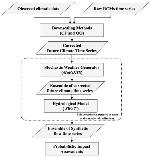
Figure 1.
Schematic representation of the proposed approach.
2.1. Study Area
The South Nation Watershed (SNW) of about 4000 in Eastern Ontario was used as a showcase. It is characterized by multigauge climatic data (from St. Albert, Russell, Morrisburg, and South Mountains metrological stations) and downstream daily discharge data (collected at Plantagenet gauging station (ID: 02LB005)) (Figure 2). Hydrogeological investigations have indicated that an impermeable overburden watershed and a lack of streambed gradients in parts of the South Nation River pose a prominent flooding risk [26]. The average maximum and minimum air temperatures are 11.5 and 1.2 °C, respectively, with a mean annual precipitation of around 1000 mm. A more detailed description of the watershed has been presented previously [27].
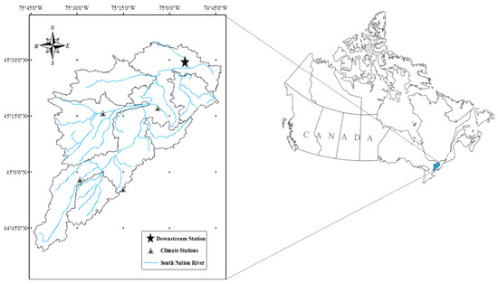
Figure 2.
Map of the South Nation Watershed.
2.2. Regional Climate Model Data
The availability of daily climatic variables at fine spatial scales is essential for hydrological impact studies [28]. The gridded daily data of precipitation, maximum near-surface air temperature, and minimum near-surface air temperature were extracted from the North American domain of Coordinated Regional Climate Downscaling Experiment (NA-CORDEX) project archive, driven by state-of-the-art GCMs as part of the the Coupled Model Inter-comparison Project Phase 5 (CMIP5) experiment (Table 1). The CORDEX project was initiated by the World Climate Research Program (WCRP) to provide reliable predictions of regional future climate change. The four independent models were forced with medium- to high-emission scenarios RCP4.5 and RCP8.5 (resulting in 8 different projections). They are originally based on outputs from the CanESM2 and EC-EARTH Global Circulation Models, whose outputs are downscaled with three Regional Climate Models: CanRCM4, RCA4, and HIRHAM5. The horizontal spatial resolution was chosen to be NAM-44 (North American domain at 0.44° horizontal grid resolution or approximately 50 km).

Table 1.
List of Regional Climate Models used in the study.
2.3. Downscaling Methods
Downscaling is a procedure undertaken to reconcile the large-scale data representativeness of observations and produce climate change data at a finer resolution. This study makes use of two statistical downscaling techniques—namely Change Factors (CF) and Quantile-Quantile transformation (QQ)—to produce more reliable station-level climatic information to be used later as inputs to a distributed impact model.
The linear correction method applied in this study, namely CF, requires three time series: observations (or synthetic climate series), historical, and future raw RCM data. The primary assumption in this method is that the relationship between historical and future projections is the same as the relation between historical RCM data and observed time series. However, the Quantile-Quantile method applies a different concept that is based on the distribution of raw simulations and observations. For a given variable, downscaling is conducted using a monthly time-step. Observed precipitation and temperature variables of 30 years (1981 to 2010) were used to define a reference climatology and to spatially downscale the coarse-scale climate data in the future (2071–2100).
2.3.1. Change Factor Method
The Change Factors (CF) method is a commonly used approach to linearly downscale a variable (e.g., precipitation) by calculating the difference between the control and future GCM simulations before scaling the baseline observations accordingly [29]. Yet, the conventional CF method is usually used a top-down approach and as such not always reliable. Nevertheless, it has been used excessively in recent climate change assessments [30,31,32,33,34,35,36,37]. The CF approach lacks the ability to correct future projections as it predicts the same variability for the future climate by keeping the same historical temporal structure, which is unrealistic [29,30,38]. One of its limitations is that it produces the exact same temporal structure of wet days (occurrences) in the future [39], which is by no means certain for a stochastic variable such as precipitation. Furthermore, extreme events that are vital in risk assessments cannot be adequately corrected by such a method when using only one observational dataset. To alleviate these disadvantages, we employed stochastic weather generators as they are capable of capturing climate variability. We explored the potential risks by producing a new set of weather data and applying factors of change obtained from raw daily RCM outputs between the reference period and the future.
Each climate station is perturbed using the simplest version of the CF method, that is, we applied the following deterministic transformation to downscaled climate model outputs:
where is the perturbed RCM output, is the original RCM output, and denotes the observed data. Analogously for temperature, we use:
where is the perturbed RCM output, is the original RCM output, and is the observed climate. The expectation is that after transformation, the means of and will each be closer to the respective means of and over the reference period.
2.3.2. Quantile-Quantile Transformation
Quantile-Quantile (QQ) transformation is an empirical routine applied to correct systematic errors in regional climate models [33,40,41]. The raw RCM outputs typically do not have the same distribution as the observations [42], and both distributions must be reconciled. It is more sophisticated than mean-based methods, and its procedure includes remapping the probability density function (PDF) of uncorrected RCM data onto the PDF of observations. Corrected RCM simulations, , of the future are produced by applying the following transformation to their cumulative distribution functions (F):
where refers to the climate variable extracted from raw RCM data. This technique has been proven to be more accurate for reproducing a valid agreement between the corrected and observed PDFs than the linear method discussed earlier [29,41,42,43]. However, one of the main drawbacks of the QQ technique is its inability to predict values beyond the original range of historic extremes [44], which may ultimately affect risk analysis.
2.4. Generating an Ensemble of Corrected-RCM-Like Realizations
The Change Factors and Quantile-Quantile downscaling methods lack the ability to produce more than one possible future state and underestimates the impact variability [45]. The variability issue is tackled in this paper by generating an ensemble of corrected RCM-like realizations, as illustrated in Figure 1, which consists of multiple runs (the number of realizations is 250) of a given stochastic weather generator fed with corrected future climate for a 30-year period. This produces a total of 2000 unique future climate projections (= 250 × 4 × 2) for each downscaling method (= 2000 × 2). Methods involving stochastic weather generators are generally capable of creating a limitless number of sequences of weather data with novel scenarios which helps with the uncertainty analysis [31]. The selection of an adequate stochastic weather generator is crucial to efficiently explore a wide range of climate risk scenarios for water resource systems [21].
This study made use of the Multi-site weather Generator of the École de Technologie Supérieure (MulGETS) [46], a multisite, multivariate weather generator that correctly reproduced historical climatic and hydrological characteristics for the SNW [27]. Wet-day precipitation sequences were reproduced using a multi-Gamma distribution (a combination of several gamma distributions). MulGETS can account for the coherency among multiple climate variables. Details of climatic data and MulGETS configuration have been previously presented in Alodah and Seidou [27]. The final result is a super-ensemble combining all ensembles containing a large number of scenarios (hereafter the “ensemble”) that inherit the trends projected by climate models while covering the range of variability from the historical period. Given that the variability range of the historical period is matched, the assumption that all scenarios are equally probable will now be more defendable.
2.5. Hydrological Response
Ultimately, the development of such new future-climate scenarios, essentially driven by corrected GCM/RCM projections, enables us to discover the risks presented by changing hydrology using altered flows at a local scale. The Soil and Water Assessment Tool (SWAT-2012) was used to simulate hydrological variables and utilizing the semi-automated SUFI-2 optimization algorithm (Sequential Uncertainty Fitting ver. 2) to evaluate the most accurate simulation based on an uncertainty analysis routine [47]. SWAT is a semi-distributed, watershed-scale hydrological model that has been extensively utilized to address water quality and quantity issues [48]. Hydrologists, conservationists, and policy makers have extensively used SWAT to predict a variety of water-related issues and their environmental impacts [48,49,50,51,52,53,54,55]. Weather information is the main physically-based input that controls the transformation of precipitation into runoff in SWAT [47].
The SNW was partitioned into 31 different Hydrologic Response Units (HRUs), each with its own land, management, and soil characteristics. A detailed description of the SWAT model configuration and parameterization used in this study has been presented previously in Alodah and Seidou [27]. A set of different statistic measures was used to assess the goodness of fit of the calibrated model, including the Nash–Sutcliffe efficiency, the RMSE-observations standard deviation ratio, and the percent bias (Table 2). Hydrological impact models, distributed models in particular (e.g., SWAT), are particularly sensitive to small-scale climate variations that might be underestimated by large-scale models [56], and it could be reasonably argued that relying on a selected few models, either in a top-down or bottom-up approach, cannot be adequately justified.
Table 2.
Goodness-of-Fit metrics used for SWAT model performance evaluation.
2.6. Quantifying the Risk Spaces
Because the goal is to build on the bottom-up approach, the same framework as Brown et al. [57] was adopted. A climate state represented by a time series is summarized by subsets of climate and hydrological statistics that are relevant to the problem under investigation. These subsets can be calculated for any observational time series or any downscaled climate model outputs. A climate state will yield a level of risk and performance that is measured by a set of risk/performance indicators. These indicators are obtained by feeding SWAT with the perturbed time series data, each of which is unique. We placed a greater focus on hydrological risks, due to their direct impacts on the watershed systems. This includes analyzing extreme values based on statistical models and investigating the timing and intensity of peak spring flow.
2.6.1. Extreme Value Statistical Probability Models (AM and 7Q)
The 3-parameter Generalized Extreme Value (GEV) and 2-parameter Weibull (WBL) distribution functions were fitted to the annual maximum streamflows (AM) and minimum extreme events (the lowest 7-day average flow, or 7Q), respectively, based on seven time-intervals (2, 5, 10, 20, 50, 100, and 500 years). The cumulative distribution functions (CDFs) of the GEV and WBL models are [58]:
where ξ, μ, and σ are the shape, location, and scale parameters, respectively. Maximum likelihood (ML) estimators, as recommended by Das et al. [59], are used to compute the parameters of these statistical models based on 95% confidence intervals (α = 0.05).
2.6.2. Spring Flow Timing and Intensity
Another important phenomenon with significant impacts on the hydrology of many river systems in temperate regions is the timing of the annual snowmelt and changes to river-ice conditions. In the SNW, the most common flooding events are caused by snowmelt-driven runoff. Hence, future changes in the spring snowmelt and river-ice breakup, particularly at high latitudes or in large mountain regions, seem inevitable. These changes in river-ice processes are useful indicators of climate change because of their sensitivity to air temperature [60,61]. Warmer winters may promote dramatic alterations in discharge patterns and in the severity and timing of the snowmelt. A threshold amount of energy, including the mean daily temperature and soil heat flux, as well as the areal coverage of snow are critical in controlling the release of the stored water. In the SWAT model, the snowmelt starts when the daily maximum temperature (SMTMP) is above 0 °C and its uniformly released water is considered to be precipitation [48]. For the sake of simplicity, the peak spring flow is defined as the event of maximum daily flow in the spring season from January 1 to May 31.
2.7. Likelihood Estimation Using KDE
It is assumed that the synthetically generated time series will be a fair representation of the natural climate variability. Using all sample data, we employed a nonparametric density estimation function, or the kernel density estimator (KDE) to build a continuous probability density function (PDF) without making any a priori assumptions with regard to the underlying distribution. This approach involves exploring the extent of possible changes to hydroclimatic variables in the context of climate change. This includes analyzing the main characteristics of hydrological variables. The kernel density estimator of a sample of a d-variate random vector (, , …, ), drawn from an unknown distribution, is given by:
where K is a non-negative kernel smoothing function, and h the non-negative bandwidth. The bivariate kernel density estimation in this study was based on a diagonal bandwidth matrix and a Gaussian kernel [62].
3. Results
3.1. SWAT Calibration and Validation
The results of the proposed method for the South Nation Watershed under changing climate conditions using a stochastic data-oriented approach are presented. Applying the two downscaling methods described above to different CORDEX data with corrected daily time series of precipitation, maximum and minimum temperature from four RCMs under the conditions of RCP4.5 and RCP8.5 emission scenarios were generated for every metrological station. The SWAT model was calibrated with 15 years of observed streamflow at a monthly resolution for the period from Jan. 1981 to Dec. 1995 and validated on the period from Jan. 1996 to Dec. 2005. Table 3 provides results of a set of statistics that show a satisfactory agreement between observed and simulated streamflows in both periods.
Table 3.
SWAT model performance in the calibration and validation periods.
3.2. Time Series Generation for the Reference and Future Periods
The weather generator, MulGETS, was used to generate 250 30-year climate datasets for each climate scenario. Then, the SWAT model, calibrated on historical climate data, was forced with the corrected future climate information to investigate hydrological changes. This resulted in 4000 realizations of future daily streamflow sequences, each consisting of 30 years of predictions. The exact number of simulations is presented in Table 4. To account for uncertainties, the total of 480,000 years of predictions are summarized using extreme-streamflow indicators that describe the associated risks and allow for comparisons against observations.
Table 4.
Details of models and number of future predictions used in the study.
3.3. Representation of the Sensitivity Space
3.3.1. Flood and Drought Indicators
Hydrologically-based extreme streamflow metrics simulated by SWAT, including the design flood and 7-day low flow based on selective return periods, were analyzed. These results were compared to the equivalent SWAT-estimated extreme indices on the historical period to quantify possible changes (Figure 3). The isolines in Figure 3 depict the intensity of projections as the probability scale is given by the colour varying smoothly from yellow (higher intensity) to blue (less intensity). The analysis of both datasets showed that flooding events will be affected more than low flow extremes, presumably due to predicted changes in the duration of snow cover. Results of the ensemble (Figure 3e) imply significant decreases in the annual maximum flows and increasing summer minimum flows by mostly all data configurations (i.e., RCMs, RCPs, and downscaling methods).
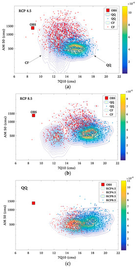
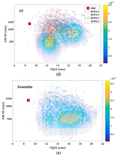
Figure 3.
Bivariate kernel density estimations of the 50-year flooding event (AM 50) and the 7-day low flow of 10-year return period (7Q10) based on (a) RCP4.5 and (b) RCP8.5 scenarios, derived from ensembles of downscaled climate data using (c) QQ method, (d) CF method, and (e) the ensemble of all simulations. Each point represents a hydrological response to a climate-change realization (projection), and isolines represent their probability where isoline-values coded by color from yellow (higher intensity) to blue (less intensity). Results are compared to observed data (red square).
Further analysis was conducted on extreme values by combining all simulations by each downscaling method, resulting in 30,000 years of simulated streamflow data. Drought indices (7Q) and design floods (AM) of these time series were compared to observed ones (Figure 4). The comparison indicates that higher air temperatures lead to reduced summer low-flows and less intense high flows. The ensemble results indicate similar trends in both indices—fewer droughts and extreme flooding events.
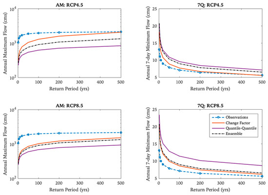
Figure 4.
Estimations of future drought indices (7Q) and design floods (AM) based on RCP4.5 and RCP8.5 constructed from prolonged corrected climate time series, compared to observed and ensemble series.
3.3.2. Spring Flow Variability
Increasing temperatures have a direct effect on the hydrology of the watershed by changing to the snowmelt-driven runoff that occurs in late winter/early spring. Shorter duration of snowpack and an increase in stream flow in the winter are projected, triggered by a warming winter, particularly in cold regions. This is predicted by most models and scenarios with some variations in timing and magnitude of the largest flow with more substantial warming occurring in the winter months. Figure 5 shows the disparity between the timing of the largest flow in the historical period and in the late-21st century. Between 1981 and 2010, the median date of the largest spring flow was March 12th (red dashed line in Figure 5b). The domination of most of the models and downscaling methods suggests that the peak spring flow will occur earlier, which is consistent with an earlier spring warming. As a result, the intensity of the annual spring flow at the outlet of the SNW is expected to significantly decrease by up to 60% (Figure 5a). The ensemble results suggest a 50% decrease in the quantity and the occurrence of the peak spring flow to be before the month of March.
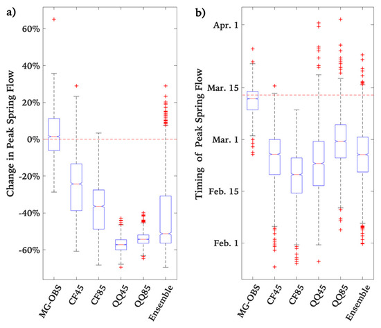
Figure 5.
Estimations Projected changes in (a) the magnitude (%) and (b) timing of the peak spring flow event at the outlet of the SNW using two downscaling methods (Change Factor {CF}, and Quantile-Quantile method {QQ}) and forced with two climate scenarios (RCP4.5 {45} and RCP8.5 {85}). “Ensemble” represents all simulations combined and compared to the range of variability observed in the reference period (MG-OBS).
4. Discussion
The main contribution of this paper is to represent the variability of future outcomes through ensembles of realizations of climate time series that are converted into ensemble of impacts. The spread of these ensembles is a representation of the uncertainty in future climate and impacts. The uncertainty comes from the fact that there is no consensus approximation of climate response to a doubling of atmospheric carbon dioxide (or climate sensitivity) although the initial estimation by National Academy of Sciences in 1979 [65] to be in the range of 1.5–4.5 °C was still adopted by the recent reports of the Intergovernmental Panel on Climate Change (IPCC) [66,67]. Andrews et al. [68] suggested that the response of global temperature might be greater and more uncertain than previously estimated, specifically at the upper end. The ensemble also covers the range of variability observed during the baseline period. The spread of the ensemble depends on the climate model, emission scenario and the choice of downscaling methods. The following sections discuss the impacts of these factors on the results.
4.1. Comparison of Downscaling Methods
By comparing downscaling methods in Figure 3 and Figure 5, it becomes apparent that the QQ technique outperformed the mean-based CF by correcting the distributions of RCM data rather than a single statistic. The cloud of points is denser (yellow contours) where the probability is higher. QQ outcomes have a tendency to consistent clouds representing different climate models and scenarios. Indeed, the convergence in the projected QQ results across RCMs with different parameterization and climate sensitivity may suggest a more refined and skillful representation of future climate and hydrological systems, especially in the estimation of extreme daily precipitation [42]. However, in the context of risk analysis, Daniels et al. [69] stated that one cannot utterly exclude an outlier scenario as it may characterize some underlying physical processes that were missed by other models or scenarios.
The mean-based downscaling method used in this study provides more diverse results (Figure 3). Results, however, are scattered, suggesting that the choice of the downscaling method will greatly affect the estimated impacts and thus adaptation strategies. In the absence of evidence that one method is better than another, the safest approach is to use all available methods. Several researchers or practitioners use one downscaling method without justification, neglecting that their results will be tainted by that choice. Research is needed to assess the relative credibility of downscaling methods in order to choose the most reliable approach.
4.2. Sensitivity Domains Assessment
Based on the probabilistic assessment of climate change, the 7-day mean annual minima and annual maxima indices suggested positive changes in the future period compared to the reference period. While low streamflow is a product of a complex combination of several factors in the physical processes, a possible reason of such projected changes in low flow is attributed to enhanced evapotranspiration (due to increased air temperature) from the wet-land surfaces of the watershed in summer [70], which leads to increased precipitation frequency through more intense convective storms and consequently increasing flows during the summer months. These projected changes of volume in low flows would be welcome especially in terms of their impacts on aquatic habitat and water quality.
Higher values of future low flows compared to the baseline period due to increased rainfall intensity in North America were reported by Shrestha et al. [71] based on SWAT simulations forced by data from ten GCMs from CMIP5 archives in response to RCP4.5 and RCP8.5 scenarios in a river located in southwest Ohio, USA. Similar conclusions of extremely low flow conditions to occur less frequently in the future were reported by modeling studies applied to different watersheds across Europe [72,73] and Asia [74,75]. In fact, these projections are also in agreement with previously reported findings of upward trends in observed low flow values across Canada [76,77]. For example, Khaliq et al. [78] investigated observed values of 1-, 7-, 15-, and 30-day annual low-flow indicators in some Canadian rivers and found significantly increasing trends in southern Ontario. Similarly, Moore et al. [79] found a statistically large positive trend in streamflow during low flow season in southwest British Columbia. Moreover, Novotny and Stefan [80] found 7-day low flows to be increasing at a significant rate in three major river basins of Minnesota during both the summer and winter. In general, both low- and high-flows have been investigated in various regional studies, with no consistent conclusions in terms of how they will be altered by climate change [21]. Rather, it is believed that such extremes are very localized and dependent on the selected GCMs and hydrological models; thus results cannot be simply generalized.
On the other hand, spring peak flow is generally a product of average air temperature and snowmelt runoff. Most of the ensemble data suggest an early occurrence of peak spring flow. This result is consistent with the finding of Gunawardhana and Kazama [72], who projected an early occurrence of peak spring flow in Italy by approximately 12 days during the 2080s in comparison to the baseline period. Also, it is supported by observed and projected changes in spring streamflow-timing across parts of western North America [81]. An advance in the timing of spring peak flow could negatively affect water supply, ecosystem, and reservoirs’ storage management [81]. However, such change in timing implies a reduction in snowmelt runoff severity (and hence the magnitude of the largest daily mean flows in spring), and the economic impacts will be apparent particularly in Canada [82]. These findings can likely explain the projected reduction in annual maxima values in a mainly snowmelt dominated river, where typically the highest flow occurs in early spring each year caused by snowmelt-generated runoff. These results are also consistent with previous works done in some Canadian watersheds that detected the same behaviour in the past such as Zhang et al. [83].
When multiple RCMs and downscaling approaches are used, the best hydrological estimate can be constructed based on weighting of combined results of rainfall-runoff modelling. By adopting the versatile methodology considered herein, it is believed that the risk of extremes and their consequent losses under an uncertain climate can be significantly reduced, as risk cannot be completely eliminated. Ideally, further improvement to the super-ensemble can be achieved by considering more stochastic weather generators, climate-change models, and downscaling methods to ensure a thorough evaluation. To overcome the high computational requirements to construct the super-ensemble, further research is needed to determine the optimal length of the chain containing realizations needed to represent observed data in climatic and hydrological modelling.
5. Conclusions
This paper proposed a novel approach to associate a credibility measure to the climate and sensitivity measure in the bottom-up approach by combining synthetically generated climate series with downscaled climate model output to populate the climate and sensitivity spaces. The large number of projections allowed us to quantify future uncertainties and provided better coverage of the risk space based on probabilistic assessment of climate change. Furthermore, the likelihood measure provides a more practical assessment of the plausibility of future risks to serve infrastructure design and allow more confidence in water-related management decisions. Ideally, the generation of such ensembles should contain—to a feasible extent—as many uncertainty elements as possible. Given that the choice of climate models, downscaling techniques, and weather generator affects the results, a super-ensemble of future climate series was used to derive flooding and drought indices, while bearing in mind the uncertainties inherent in the extreme value modelling under a changing climate at regional scales. The results of the modelled risk analysis on the South Nation Watershed located in Ontario, Canada, indicate a marginal increase in the 7-day low flow, whereas design floods will noticeably weaken. A shorter and warmer winter is expected to result in an earlier disappearance of accumulated winter snow cover, an early onset of snowmelt, and consequently an earlier and less intensive peak spring flow. While an application was centered in one pilot watershed, the methodology delivers new insights into hydrological processes under changing climate conditions in general and will be of interest for Canada and beyond. The need is also manifest for examining a broader range of hydrologic indicators. Finally, the broader natural uncertainty posed by climate change and land use, and their implicit disruptions to various agro-socioeconomic and water sectors at an operational level, may constitute an interesting and worthwhile extension of this study.
Author Contributions
A.A. and O.S. conceived and designed the study. A.A. collected the data, performed the computations, analyzed the results and wrote the original draft of the manuscript. O.S. supervised the research work and contributed to the interpretation of the results, and manuscript revision.
Funding
The research was partially funded by the National Sciences and Engineering Research Council discovert grant (RGPIN/ 2016-05094) to the second author.
Conflicts of Interest
The authors declare no conflict of interest.
References
- Stocker, T.F.; Qin, D.; Plattner, G.-K.; Tignor, M.; Allen, S.K.; Boschung, J.; Nauels, A.; Xia, Y.; Bex, V.; Midgley, P.M. Climate Change 2013: The Physical Science Basis. Intergovernmental Panel on Climate Change, Working Group I Contribution to the IPCC Fifth Assessment Report (AR5); Cambridge University Press: New York, NY, USA, 2013; pp. 159–254. [Google Scholar]
- Manabe, S. Climate and the ocean circulation: I. The atmospheric circulation and the hydrology of the earth’s surface. Mon. Weather Rev. 1969, 97, 739–774. [Google Scholar] [CrossRef]
- Gleick, P.H. Climate change, hydrology, and water resources. Rev. Geophys. 1989, 27, 329–344. [Google Scholar] [CrossRef]
- Whitfield, P.H.; Cannon, A.J. Recent variations in climate and hydrology in Canada. Can. Water Resour. J. 2000, 25, 19–65. [Google Scholar] [CrossRef]
- Arora, V.K.; Boer, G.J. Effects of simulated climate change on the hydrology of major river basins. J. Geophys. Res. Atmos. 2001, 106, 3335–3348. [Google Scholar] [CrossRef]
- Frich, P.; Alexander, L.V.; Della-Marta, P.M.; Gleason, B.; Haylock, M.; Tank, A.K.; Peterson, T. Observed coherent changes in climatic extremes during the second half of the twentieth century. Clim. Res. 2002, 19, 193–212. [Google Scholar] [CrossRef]
- Bierkens, M.F.; Dolman, A.J.; Troch, P.A. (Eds.) Climate and the Hydrological Cycle; International Association of Hydrological Sciences: Wallingford, UK, 2008; Volume 8. [Google Scholar]
- Panagoulia, D. Hydrological response of a medium-sized mountainous catchment to climate changes. Hydrol. Sci. J. 1991, 36, 525–547. [Google Scholar] [CrossRef]
- Panagoulia, D. Impacts of GISS-modelled climate changes on catchment hydrology. Hydrol. Sci. J. 1992, 37, 141–163. [Google Scholar] [CrossRef]
- Panagoulia, D.; Bárdossy, A.; Lourmas, G. Multivariate stochastic downscaling models generating precipitation and temperature scenarios of climate change based on atmospheric circulation. Glob. Nest J. 2008, 10, 263–272. [Google Scholar]
- Pielke Sr, R.A.; Wilby, R.; Niyogi, D.; Hossain, F.; Dairuku, K.; Adegoke, J.; Suding, K. Dealing with complexity and extreme events using a bottom-up, resource-based vulnerability perspective. Extreme Events and Natural Hazards: The Complexity Perspective. Geophys. Monogr. Ser. 2012, 196, 345–359. [Google Scholar]
- García, L.E.; Matthews, J.H.; Rodriguez, D.J.; Wijnen, M.; DiFrancesco, K.N.; Ray, P. Beyond Downscaling: A Bottom-up Approach to Climate Adaptation for Water Resources Management; World Bank Publications: Washington, DC, USA, 2014. [Google Scholar]
- Brown, C.; Werick, W.; Leger, W.; Fay, D. A Decision-Analytic Approach to Managing Climate Risks: Application to the Upper Great Lakes. J. Am. Water. Resour. Assoc. 2011, 47, 524–534. [Google Scholar] [CrossRef]
- Wilby, R.L. Adaptation: Wells of wisdom. Nat. Clim. Chang. 2011, 1, 302–303. [Google Scholar] [CrossRef]
- Bhave, A.; Mishra, A.; Raghuwanshi, N. A combined bottom-up and top-down approach for assessment of climate change adaptation options. J. Hydrol. 2014, 518, 150–161. [Google Scholar] [CrossRef]
- Culley, S.; Noble, S.; Yates, A.; Timbs, M.; Westra, S.; Mair, H.R.; Giuliani, M.; Castelletti, A. A bottom-up approach to identifying the operational adaptive capacity of water resources systems to a changing climate. Water Resour. Res. 2016, 52, 6751–6758. [Google Scholar] [CrossRef]
- Alodah, A.; Seidou, O. The realism of Stochastic Weather Generators in Risk Discovery. WIT Trans. Ecol. Environ. 2017, 220, 239–249. [Google Scholar] [CrossRef]
- Guo, D.; Westra, S.; Maier, H.R. Use of a scenario-neutral approach to identify the key hydro-meteorological attributes that impact runoff from a natural catchment. J. Hydrol. 2017, 554, 317–330. [Google Scholar] [CrossRef]
- Seidou, O.; Alodah, A. From top-down to bottom-up approaches to risk discovery: a paradigm shift in climate change impacts and adaptation studies related to the water sector. In Proceedings of the Annual Conference of the Canadian Society for Civil Engineering (CSCE2018), Fredericton, NB, Canada, 13–16 June 2018. DM36-01-11. [Google Scholar]
- Panagoulia, D. Artificial neural networks and high and low flows in various climate regimes. Hydrol. Sci. J. 2006, 51, 563–587. [Google Scholar] [CrossRef]
- Sapač, K.; Medved, A.; Rusjan, S.; Bezak, N. Investigation of Low- and High-Flow Characteristics of Karst Catchments under Climate Change. Water 2019, 11, 925. [Google Scholar] [CrossRef]
- Tharme, R.E. A global perspective on environmental flow assessment: Emerging trends in the development and application of environmental flow methodologies for rivers. River Res. Appl. 2003, 19, 397–441. [Google Scholar] [CrossRef]
- Arthington, A.H.; Bunn, S.E.; Poff, N.L.; Naiman, R.J. The challenge of providing environmental flow rules to sustain river ecosystems. Ecol. Appl. 2006, 16, 1311–1318. [Google Scholar] [CrossRef]
- Linnansaari, T.; Monk, W.A.; Baird, D.J.; Curry, R.A. Review of approaches and methods to assess Environmental Flows across Canada and internationally. DFO Can. Sci. Advis. Secr. Res. Doc. 2012, 39, 1–74. [Google Scholar]
- Pastor, A.V.; Ludwig, F.; Biemans, H.; Hoff, H.; Kabat, P. Accounting for environmental flow requirements in global water assessments. Hydrol. Earth Syst. Sci. 2014, 18, 5041–5059. [Google Scholar] [CrossRef]
- Chin, V.I.; Wang, K.T.; Vallery, O.J. Water Resources of the South Nation River Basin; Rep. No. 13; Ontario Ministry of the Environment, Water Resources Branch: Toronto, ON, Canada, 1980. [Google Scholar]
- Alodah, A.; Seidou, O. The adequacy of stochastically generated climate time series for water resources systems risk and performance assessment. Stoch. Environ. Res. Risk Assess. 2019, 33, 253–269. [Google Scholar] [CrossRef]
- Semenov, V.A. Structure of temperature variability in the high latitudes of the Northern Hemisphere. Izv. Atmos. Ocean. Phys. 2007, 43, 687–695. [Google Scholar] [CrossRef]
- Lenderink, G.; Buishand, A.; Deursen, W.V. Estimates of future discharges of the river Rhine using two scenario methodologies: Direct versus delta approach. Hydrol. Earth Syst. Sci. 2007, 11, 1145–1159. [Google Scholar] [CrossRef]
- Diaz-Nieto, J.; Wilby, R.L. A comparison of statistical downscaling and climate change factor methods: Impacts on low flows in the River Thames, United Kingdom. Clim. Chang. 2005, 69, 245–268. [Google Scholar] [CrossRef]
- Hansen, C.H.; Goharian, E.; Burian, S. Downscaling precipitation for local-scale hydrologic modeling applications: Comparison of traditional and combined change factor methodologies. J. Hydrol. Eng. 2017, 22, 04017030. [Google Scholar] [CrossRef]
- Harris, C.N.P.; Quinn, A.D.; Bridgeman, J. The use of probabilistic weather generator information for climate change adaptation in the UK water sector. Meteorol. Appl. 2014, 21, 129–140. [Google Scholar] [CrossRef]
- Lafon, T.; Dadson, S.; Buys, G.; Prudhomme, C. Bias correction of daily precipitation simulated by a regional climate model: A comparison of methods. Int. J. Climatol. 2013, 33, 1367–1381. [Google Scholar] [CrossRef]
- Luo, M.; Liu, T.; Frankl, A.; Duan, Y.; Meng, F.; Bao, A.; De Maeyer, P. Defining spatiotemporal characteristics of climate change trends from downscaled GCMs ensembles: How climate change reacts in Xinjiang, China. Int. J. Climatol. 2018, 38, 2538–2553. [Google Scholar] [CrossRef]
- Mpelasoka, F.S.; Chiew, F.H.S. Influence of rainfall scenario construction methods on runoff projections. J. Hydrometeorol. 2009, 10, 1168–1183. [Google Scholar] [CrossRef]
- Teutschbein, C.; Seibert, J. Bias correction of regional climate model simulations for hydrological climate-change impact studies: Review and evaluation of different methods. J. Hydrol. 2012, 456, 12–29. [Google Scholar] [CrossRef]
- Van Roosmalen, L.; Sonnenborg, T.O.; Jensen, K.H.; Christensen, J.H. Comparison of hydrological simulations of climate change using perturbation of observations and distribution-based scaling, Soil Science Society of America. Vadose Zone J. 2011, 10, 136–150. [Google Scholar] [CrossRef]
- Hayhoe, K.A. A Standardized Framework for Evaluating the Skill of Regional Climate Downscaling Techniques. Ph.D. Thesis, University of Illinois at Urbana-Champaign, Champaign County, IL, USA, 2010. [Google Scholar]
- Seidou, O.; Ramsay, A.; Nistor, I. Climate change impacts on extreme floods II: Improving flood future peaks simulation using non-stationary frequency analysis. Nat. Hazards 2012, 60, 715–726. [Google Scholar] [CrossRef]
- Maraun, D. Bias correcting climate change simulations-a critical review. Curr. Clim. Chang. Rep. 2016, 2, 211–220. [Google Scholar] [CrossRef]
- Themβel, M.J.; Gobiet, A.; Leuprecht, A. Empirical statistical downscaling and error correction of daily precipitation from regional climate models. Int. J. Climatol. 2010, 31, 1530–1544. [Google Scholar] [CrossRef]
- Sarr, M.A.; Seidou, O.; Tramblay, Y.; El Adlouni, S. Comparison of downscaling methods for mean and extreme precipitation in Senegal. J. Hydrol. Reg. Stud. 2015, 4, 369–385. [Google Scholar] [CrossRef]
- Angelina, A.; Gado Djibo, A.; Seidou, O.; Seidou Sanda, I.; Sittichok, K. Changes to flow regime on the Niger River at Koulikoro under a changing climate. Hydrol. Sci. J. 2015, 60, 1709–1723. [Google Scholar] [CrossRef]
- Wilby, R.L.; Fowler, H.J. Regional Climate Downscaling: Modelling the Impact of Climate Change on Water Resources; Fung, F., Lopez, A., New, M., Eds.; Wiley-Blackwell: Chichester, West Sussex, UK; Hoboken, NJ, USA, 2011; ISBN 978-1-4051-9671-0. [Google Scholar]
- Wilks, D.S. Multi-site generalization of a daily stochastic precipitation model. J. Hydrol. 1998, 210, 178–191. [Google Scholar] [CrossRef]
- Chen, J.; Brissette, F.P.; Zhang, X.J. A multi-site stochastic weather generator for daily precipitation and temperature. Trans. ASABE 2014, 57, 1375–1391. [Google Scholar]
- Abbaspour, K.C.; Yang, J.; Maximov, I.; Siber, R.; Bogner, K.; Mieleitner, J.; Srinivasan, R. Modelling hydrology and water quality in the pre-alpine/alpine Thur watershed using SWAT. J. Hydrol. 2007, 333, 413–430. [Google Scholar] [CrossRef]
- Neitsch, S.L.; Arnold, J.G.; Kiniry, J.R.; Williams, J.R. Soil and Water Assessment Tool Theoretical Documentation Version 2009; Texas Water Resources Institute: College Station, TX, USA, 2011. [Google Scholar]
- Srinivasan, R.; Arnold, J.G. Integration of a basin-scale water quality model with GIS. Water Resour. Bull. 1994, 30, 453–462. [Google Scholar] [CrossRef]
- Arnold, J.G.; Srinivasan, R.; Muttiah, R.S.; Williams, J.R. Large area hydrologic modeling and assessment part I: Model development 1. J. Am. Water. Resour. Assoc. 1998, 34, 73–89. [Google Scholar] [CrossRef]
- White, K.L.; Chaubey, I. Sensitivity analysis, calibration, and validations for a multisite and multivariable SWAT model. J. Am. Water. Resour. Assoc. 2005, 41, 1077–1089. [Google Scholar] [CrossRef]
- Tuppad, P.; Douglas-Mankin, K.R.; Lee, T.; Srinivasan, R.; Arnold, J.G. Soil and Water Assessment Tool (SWAT). hydrologic/water quality model: Extended capability and wider adoption. Trans. ASABE 2011, 54, 1677–1684. [Google Scholar] [CrossRef]
- Arnold, J.G.; Moriasi, D.N.; Gassman, P.W.; Abbaspour, K.C.; White, M.J.; Srinivasan, R.; Santhi, C.; Harmel, R.D.; Van Griensven, A.; Van Liew, M.W.; et al. SWAT: Model use, calibration, and validation. Trans. ASABE 2012, 55, 1491–1508. [Google Scholar] [CrossRef]
- Santhi, C.; Arnold, J.; Williams, J.; Dugas, W.; Srinivasan, R.; Hauck, L. Validation of the SWAT model on a large river basin with point and nonpoint sources 1. J. Am. Water. Resour. Assoc. 2001, 37, 1169–1188. [Google Scholar] [CrossRef]
- Tan, M.L.; Gassman, P.W.; Srinivasan, R.; Arnold, J.G.; Yang, X. A Review of SWAT Studies in Southeast Asia: Applications, Challenges and Future Directions. Water 2019, 11, 914. [Google Scholar] [CrossRef]
- Wilby, R.L.; Charles, S.P.; Zorita, E.; Timbal, B.; Whetton, P.; Mearns, L.O. Guidelines for Use of Climate Scenarios Developed from Statistical Downscaling Methods; Supporting material of the Intergovernmental Panel on Climate Change; DDC of IPCC TGCIA: Geneva, Switzerland, 2004. [Google Scholar]
- Brown, C.; Ghile, Y.; Laverty, M.; Li, K. Decision scaling: Linking bottom up vulnerability analysis with climate projections in the water sector. Water Resour. Res. 2012, 48, 9537. [Google Scholar] [CrossRef]
- Jenkinson, A.F. The frequency distribution of the annual maximum (or minimum) values of meteorological elements. Q. J. R. Meteorol. Soc. 1955, 81, 158–171. [Google Scholar] [CrossRef]
- Das, S.; Millington, N.; Simonovic, S.P. Distribution choice for the assessment of design rainfall for the city of London (Ontario, Canada) under climate change. Can. J. Civ. Eng. 2013, 40, 121–129. [Google Scholar] [CrossRef]
- Huntington, T.G.; Hodgkins, G.A.; Dudley, R.W. Historical trend in river ice thickness and coherence in hydroclimatological trends in Maine. Clim. Chang. 2003, 61, 217–236. [Google Scholar] [CrossRef]
- Karl, T.R.; Groisman, P.Y.; Knight, R.W.; Heim, R.R., Jr. Recent variations of snow cover and snowfall in North America and their relation to precipitation and temperature variations. J. Clim. 1993, 6, 1327–1344. [Google Scholar] [CrossRef]
- Botev, Z.I.; Grotowski, J.F.; Kroese, D.P. Kernel density estimation via diffusion. Ann. Stat. 2010, 38, 2916–2957. [Google Scholar] [CrossRef]
- Liew, M.W.; Veith, T.L.; Bosch, D.D.; Arnold, J.G. Suitability of SWAT for the conservation effects assessment project: A comparison on USDA-ARS experimental watersheds. J. Hydrol. Eng. 2007, 12, 173–189. [Google Scholar] [CrossRef]
- Moriasi, D.N.; Arnold, J.G.; Van Liew, M.W.; Bingner, R.L.; Harmel, R.D.; Veith, T.L. Model evaluation guidelines for systematic quantification of accuracy in watershed simulations. Trans. ASABE 2007, 50, 885–900. [Google Scholar] [CrossRef]
- National Academy of Sciences. Carbon Dioxide and Climate: A Scientific Assessment; National Academy of Sciences: Washington, DC, USA, 1979. [Google Scholar]
- IPCC. 2007: Climate Change 2007: Synthesis Report. Contribution of Working Groups I, II and III to the Fourth Assessment Report of the Intergovernmental Panel on Climate Change; Cre Writing Team, Pachauri, R.K., Reisinger, A., Eds.; IPCC: Geneva, Switzerland, 2007; 104p. [Google Scholar]
- IPCC. 2014: Climate Change 2014: Impacts, Adaptation, and Vulnerability. Part A: Global and Sectoral Aspects. Contribution of Working Group II to the Fifth Assessment Report of the Intergovernmental Panel on Climate Change; Field, C.B., Barros, V.R., Dokken, D.J., Mach, K.J., Mastrandrea, M.D., Bilir, T.E., Chatterjee, M., Ebi, K.L., Estrada, Y.O., Genova, R.C., et al., Eds.; Cambridge University Press: Cambridge, UK; New York, NY, USA, 2014; 1132p. [Google Scholar]
- Andrews, T.; Gregory, J.M.; Paynter, D.; Silvers, L.G.; Zhou, C.; Mauritsen, T.; Titchner, H. Accounting for changing temperature patterns increases historical estimates of climate sensitivity. Geophys. Res. Lett. 2018, 45, 8490–8499. [Google Scholar] [CrossRef]
- Daniels, A.E.; Morrison, J.F.; Joyce, L.A.; Crookston, N.L.; Chen, S.C.; McNully, S.G. Climate Projections FAQ; General Technical Report; Department of Agriculture, Forest Service, Rocky Mountain Research Station: Fort Collins, CO, USA, 2012; pp. 1–32. [Google Scholar]
- Abdel-Fattah, S.; Krantzberg, G. A review: Building the resilience of Great Lakes beneficial uses to climate change. Sustain. Water Qual. Ecol. 2014, 3, 3–13. [Google Scholar] [CrossRef]
- Shrestha, S.; Sharma, S.; Gupta, R.; Bhattarai, R. Impact of global climate change on stream low flows: A case study of the great Miami river watershed, Ohio, USA. Int. J. Agric. Biol. Eng. 2019, 12, 84–95. [Google Scholar] [CrossRef]
- Gunawardhana, L.N.; Kazama, S. A water availability and low-flow analysis of the Tagliamento River discharge in Italy under changing climate conditions. Hydrol. Earth Syst. Sci. 2012, 16, 1033–1045. [Google Scholar] [CrossRef]
- Laaha, G.; Parajka, J.; Viglione, A.; Koffler, D.; Haslinger, K.; Schöner, W.; Zehetgruber, J.; Blöschl, G. A three-pillar approach to assessing climate impacts on low flows. Hydrol. Earth Syst. Sci. 2016, 20, 3967–3985. [Google Scholar] [CrossRef]
- Gain, A.K.; Immerzeel, W.W.; Sperna Weiland, F.C.; Bierkens, M.F.P. Impact of climate change on the stream flow of the lower Brahmaputra: Trends in high and low flows based on discharge-weighted ensemble modelling. Hydrol. Earth Syst. Sci. 2011, 15, 1537–1545. [Google Scholar] [CrossRef]
- Tian, Y.; Xu, Y.P.; Ma, C.; Wang, G. Modeling the impact of climate change on low flows in Xiangjiang River Basin with Bayesian averaging method. J. Hydrol. Eng. 2017, 22, 04017035. [Google Scholar] [CrossRef]
- Ehsanzadeh, E.; Adamowski, K. Detection of trends in low flows across Canada. Can. Water Resour. J. 2007, 32, 251–264. [Google Scholar] [CrossRef]
- Yue, S.; Pilon, P.; Phinney, B.O.B. Canadian streamflow trend detection: Impacts of serial and cross-correlation. Hydrol. Sci. J. 2003, 48, 51–63. [Google Scholar] [CrossRef]
- Khaliq, M.N.; Ouarda, T.B.; Gachon, P.; Sushama, L. Temporal evolution of low-flow regimes in Canadian rivers. Water Resour. Res. 2008, 44. [Google Scholar] [CrossRef]
- Moore, R.D.; Allen, D.M.; Stahl, K. Climate Change and Low Flows: Influences of Groundwater and Glaciers; Final Report for Climate Change Action Fund Projec A; Hydrology Applications Group, Environment Canada: Vancouver, BC, Canada, 2007; Volume 875, p. 211. [Google Scholar]
- Novotny, E.V.; Stefan, H.G. Stream flow in Minnesota: Indicator of climate change. J. Hydrol. 2007, 334, 319–333. [Google Scholar] [CrossRef]
- Stewart, I.T.; Cayan, D.R.; Dettinger, M.D. Changes in snowmelt runoff timing in western North America under abusiness as usual’climate change scenario. Clim. Chang. 2004, 62, 217–232. [Google Scholar] [CrossRef]
- Beltaos, S. Advances in river ice hydrology. Hydrol. Process. 2000, 14, 1613–1625. [Google Scholar] [CrossRef]
- Zhang, X.; Harvey, K.D.; Hogg, W.D.; Yuzyk, T.R. Trends in Canadian streamflow. Water Resour. Res. 2001, 37, 987–998. [Google Scholar] [CrossRef]
© 2019 by the authors. Licensee MDPI, Basel, Switzerland. This article is an open access article distributed under the terms and conditions of the Creative Commons Attribution (CC BY) license (http://creativecommons.org/licenses/by/4.0/).