A Study on Climate-Driven Flash Flood Risks in the Boise River Watershed, Idaho


Abstract
1. Introduction
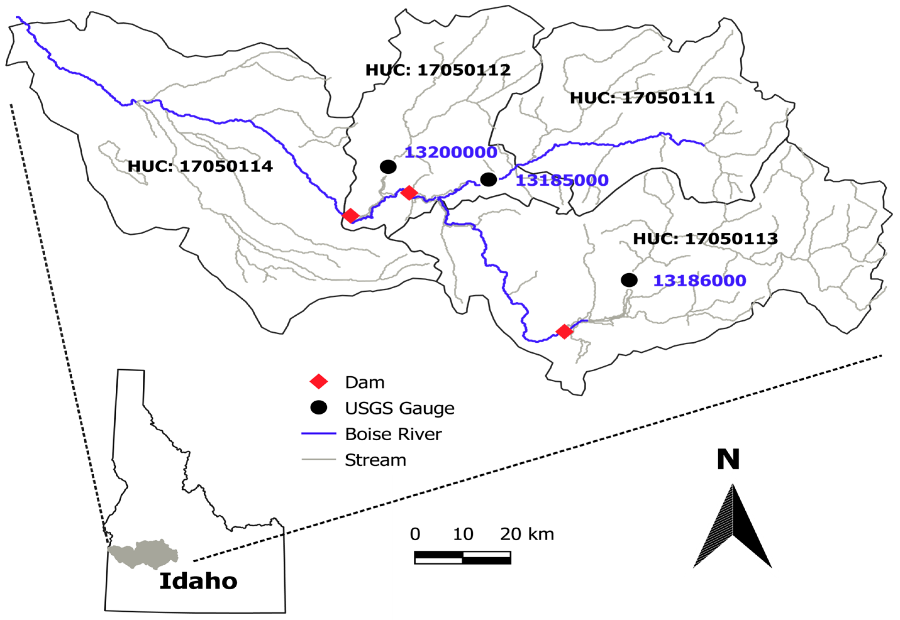
2. Study Area
3. Methodology
3.1. Flash Flood Frequency
3.2. Hydrological Model Used
3.3. Future Climate Scenarios Implemented
4. Results
5. Conclusions
Author Contributions
Funding
Conflicts of Interest
Appendix A
References
- Das, T.; Maurer, E.P.; Pierce, D.W.; Dettinger, M.D.; Cayan, D.R. Increasing in flood magnitudes in California under warming climates. J. Hydrol. 2013, 501, 101–110. [Google Scholar] [CrossRef]
- Elsner, M.M.; Cuo, L.; Voisin, N.; Deems, J.S.; Hamlet, A.F.; Vano, J.A.; Mickelson, K.E.B.; Lee, S.Y.; Lettenmaier, D.P. Implications of 21st century climate change for the hydrology of Washington State. Clim. Chang. 2010, 102, 225–260. [Google Scholar] [CrossRef]
- Wahl, T.; Jain, S.; Bender, J.; Meyers, S.D.; Luther, M.E. Increasing risk of compound flooding from strom surge and rainfall for major US cities. Nat. Clim. Chang. 2015, 5, 1093–1097. [Google Scholar] [CrossRef]
- Wing, O.E.J.; Bates, P.D.; Smith, A.M.; Sampson, C.C.; Johnson, K.A.; Fargione, J.; Morefield, P. Estimates of present and future flood risk in the conterminous United States. Environ. Res. Lett. 2018, 13, 034023. [Google Scholar] [CrossRef]
- NOAA. Billion-Dollar Weather and Climate Disasters: Table of Events. 2017. Available online: https://www.ncdc.noaa.gov/billions/events/US/2017 (accessed on 28 January 2019).
- Raff, D.A.; Pruitt, T.; Brekke, L.D. A framework for assessing flood frequency based on climate projection information. Hydrol. Earth Syst. Sci. 2009, 13, 2119–2136. [Google Scholar] [CrossRef]
- Clow, D.W. Changes in the Timing of Snowmelt and Streamflow in Colorado: A Response to Recent Warming. J. Clim. 2010, 23, 2293–2306. [Google Scholar] [CrossRef]
- Safeeq, M.; Grant, G.E.; Lewis, S.L.; Tague, C.L. Coupling snowpack and groundwater dynamics to interpret historical streamflow trends in the western United States. Hydrol. Process. 2012, 27, 655–668. [Google Scholar] [CrossRef]
- NWS (National Weather Service). Advanced Hydrologic Prediction Service; 2019. Available online: https://water.weather.gov/ahps2/inundation/index.php?gage=bigi1 (accessed on 1 March 2019).
- Melillo, J.M.; Richmond, T.C.; Yohe, G.W. Climate Change Impacts in the United States: The third national climate assessment. U.S. Glob. Chang. Res. Program 2014, 841. [Google Scholar] [CrossRef]
- Zhou, Q.; Leng, G.; Peng, J. Recent changes in the occurrences and damages of floods and droughts in the United States. Water 2018, 10, 1109. [Google Scholar] [CrossRef]
- Dettinger, M.; Udall, B.; Georgakakos, A. Western water and climate change. Ecol. Appl. 2015, 24, 2069–2093. [Google Scholar] [CrossRef]
- Kim, J.J.; Ryu, J.H. Modeling hydrological and environmental consequences of climate change and urbanization in the Boise River Watershed, Idaho. J. Am. Water Resour. Assoc. 2019, 55, 133–153. [Google Scholar] [CrossRef]
- Pierce, D.W.; Cayan, D.R.; Das, T.; Maurer, E.P.; Miller, N.; Bao, Y.; Kanamitsu, M.; Yoshimura, K.; Snyder, M.A.; Sloan, L.C.; et al. The Key Role of Heavey Precipitation Events in Climate Model disagrremnts of Future Annual Precipitation Changes in California. Am. Meteorol. Soc. 2013, 26, 5879–5896. [Google Scholar]
- USBR. Chapter 2: Hydrology and Climate Assessment. In SECURE Water Act Section 9503(c)—Reclamation Climate Change and Water; United States Bureau of Reclamation: Denver, CO, USA, 2016. [Google Scholar]
- Weil, W.; Jia, F.; Chen, L.; Zhang, H.; Yu, Y. Effects of surficial condition and rainfall intensity on runoff in loess hilly area, China. J. Hydorl. 2014, 56, 115–126. [Google Scholar]
- Miller, M.L.; Palmer, R.N. Developing an Extended Streamflow Forecast for the Pacific Northwest; World Water & Environmental Resources Congress ASCE: Philadelphia, PA, USA, 2003. [Google Scholar]
- Wood, A.W.; Maurer, E.P.; Kumar, A.; Lettenmaier, D.P. Long-Range Experimental Hydrologic Forecasting for the Eastern United States. J. Geophys. Res. 2002, 107, ACL 6-1–ACL 6-15. [Google Scholar] [CrossRef]
- Ryu, J.H. Application of HSPF to the Distributed Model Intercomparison Project: Case Study. J. Hydrol. Eng. 2009, 14, 847–857. [Google Scholar] [CrossRef]
- Quintero, F.; Mantilla, R.; Anderson, C.; Claman, D.; Krajewski, W. Assessment of Changes in Flood Frequency Due to the Effects of Climate Change: Implications for Engineering Design. Hydrology 2018, 5, 19. [Google Scholar] [CrossRef]
- IDEQ. Lower Boise River Nutrient Subbasin Assessment; Idaho Department of Environmental Quality: Boise, ID, USA, 2001; pp. 18–19.
- Carlson, B. Proposal to Raise One of Three Boise River Dams Favors Anderson Ranch. Available online: https://www.capitalpress.com/state/idaho/proposal-to-raise-one-of-three-boise-river-dams-favors/article_52d1f19f-fbed-5843-9736-7cb3174b1573.html (accessed on 15 March 2019).
- Tasker, G.D. A Comparison of methods for estimating low flow characterisics of streams. J. Am. Water Resour. Assoc. 1987, 23, 1077–1083. [Google Scholar] [CrossRef]
- Loganathan, G.V. Frequency analysis of low flows. Nord. Hydrol. 1985, 17, 129–150. [Google Scholar] [CrossRef][Green Version]
- Matalas, N.C. Probability distribution of low flows, Statistical Studies in Hydrology. In Geological Survey Professional Paper 434-A; 1963. Available online: https://pubs.usgs.gov/pp/0434a/report.pdf (accessed on 1 March 2019).
- Ryu, J.H.; Lee, J.H.; Jeong, S.; Park, S.K.; Han, K. The impacts of climate change on local hydrology and low flow frequency in the Geum River Basin, Korea. Hydrol. Process. 2011, 25, 3437–3447. [Google Scholar] [CrossRef]
- Linsley, R.K.; Kohler, M.A.; Paulhus, J.L.H. Hydrology for Engineers; McGraw-Hill: New York, NY, USA, 1982. [Google Scholar]
- Stedinger, J.R.; Vogel, R.M.; Efi, F.-G. Handbook of Hydrology; Maidment, D., Ed.; McGraw-Hill: New York, NY, USA, 1993; pp. 18.12–18.13. [Google Scholar]
- Weibull, W.A. Statistical Theory of the Strength of Materials; the Royal Swedish Institute for Engineering Research: Stockholm, Swedish, 1939. [Google Scholar]
- Chow, V.T. A general formula for hydrologic frequency analysis. Trans. Am. Geophys. Union 1951, 32, 231–237. [Google Scholar] [CrossRef]
- Fisher, R.A.; Tippett, L.H.C. Limiting Forms of the Frequency Distributions of the Smalles and Largest Member of a Sample. Proc. Camb. Philos. Soc. 1928, 24, 180–190. [Google Scholar] [CrossRef]
- Hosking, J.R.M.; Wallis, J.R.; Wood, A.W. Estimation of the Generalized Extreme Value Distribution by the Method of Probability-Weighted Moments. Technometrics 1985, 27, 251–261. [Google Scholar] [CrossRef]
- Hoshi, K.; Stedinger, J.R.; Burges, S.J. Estimation of Log-Normal Quantiles: Monte Carlo Results and First-Order Approximations. J. Hydrol. 1984, 71, 1–30. [Google Scholar] [CrossRef]
- Stedinger, J.R. Fitting Log Normal Distributions to Hydrologic Data. Water Resour. Res. 1980, 16, 481–490. [Google Scholar] [CrossRef]
- Bobee, B. The Log Pearson Type 3 Distribution and Its Application in Hydrology. Water Resour. Res. 1975, 11, 681–689. [Google Scholar] [CrossRef]
- Dudula, J.; Randhir, T.O. Modeling the influence of climate change on watershed systems: Adaptation through targeted practices. J. Hydrol. 2016, 541, 703–713. [Google Scholar] [CrossRef]
- Tong, S.T.Y.; Ranatunga, T.; He, J.; Yang, T.J. Predicting plausible impacts of sets of climate and land use change scenarios on water resources. Appl. Geogr. 2012, 32, 477–489. [Google Scholar] [CrossRef]
- Stern, M.; Flint, L.; Minear, J.; Flint, A.; Wright, S. Characterizing Changes in Streamflow and Sediment Supply in the Sacramento River Basin, California, Using Hydrological Simulation Program-Fortran (HSPF). Water 2016, 8, 432. [Google Scholar] [CrossRef]
- Bicknell, B.; Imhoff, J.; Kittle, J., Jr.; Jones, T.; Donigian, A., Jr.; Johanson, R. Hydrological Simulation Program-FORTRAN: HSPF Version 12 User’s Manual; AQUA TERRA Consultants: Mountain View, CA, USA, 2001. [Google Scholar]
- Crawford, N.H.; Linsley, R.K. Digital Simulation in Hydrology: Stanford Watershed Model IV; Technical Report No. 39; Department of Civil Engineering, Stanford University: Stanford, CA, USA, 1966. [Google Scholar]
- Donigian, A.S.; Davis, H.H. User’s Manual for Agricultural Runoff Management (ARM) Model; The National Technical Information Service: Springfield, VA, USA, 1978.
- Donigian, A.S.; Crawford, N.H. Modeling Nonpoint Pollution from the Land Surface; US Environmental Protection Agency, Office of Research and Development, Environmental Research Laboratory: Washington, DC, USA, 1976.
- Donigian, A.S.; Huber, W.C.; Laboratory, E.R.; Consultants, A.T. Modeling of Nonpoint Source Water Quality in Urban and Non-urban Areas; US Environmental Protection Agency, Office of Research and Development, Environmental Research Laboratory: Washington, DC, USA, 1991.
- Donigian, A., Jr.; Bicknell, B.; Imhoff, J.; Singh, V. Hydrological Simulation Program-Frotran (HSPF). In Computer Models of Watershed Hydrology; Water Resources Publications: Highlands Ranch, CO, USA, 1995; pp. 395–442. [Google Scholar]
- Kim, J.J.; Ryu, J.H. A threshold of basin discretization for HSPF simulations with NEXRAD inputs. J. Hydrol. Eng. 2013, 19, 1401–1412. [Google Scholar] [CrossRef]
- Mitchell, K.E.; Lohmann, D.; Houser, P.R.; Wood, E.F.; Schaake, J.C.; Robock, A.; Cosgrove, B.A.; Sheffield, J.; Duan, Q.Y.; Luo, L.; et al. The multi-institution North American Land Data Assimilation System (NLDAS): Utilizaing multiple GCIP products and partners in a continental distributed hydrologicl modeling system. J. Geophys. Res. 2004, 109, D07S90. [Google Scholar] [CrossRef]
- Abatzoglou, J.T. Development of gridded surface meteorological data for ecological applications and modeling. Int. J. Climatol. 2011, 33, 121–131. [Google Scholar] [CrossRef]
- Fasano, G.; Franceschini, A. A multivariate version of the Kolmogorov-Sminov test. Mon. Not. R. Astron. Soc. 1987, 225, 155–170. [Google Scholar] [CrossRef]
- Benjamin, J.R.; Cornell, C.A. Probability, Statistics and Decision for Civil Engineers; McGraw-Hill: New York, NY, USA, 1970; 684p. [Google Scholar]
- Kite, G.W. Confidence limits for design events. Water Resour. Res. 1975, 11, 48–53. [Google Scholar] [CrossRef]
- Duda, P.B.; Hummel, P.R.; Donigian, A.S., Jr.; Imhoff, J.C. BASINS/HSPF: Model use, calibration, and validation. Trans. ASABE 2012, 55, 1523–1547. [Google Scholar] [CrossRef]
- Moriasi, D.N.; Arnold, J.G.; Van Liew, M.W.; Binger, R.L.; Harmel, R.D.; Veith, T.L. Model Evaluation Guidelines for Systematic Quantification of Accuracy in Watershed Simulations. Am. Soc. Agric. Biol. Eng. 2007, 50, 885–900. [Google Scholar] [CrossRef]
- Milly, P.C.D.; Betancourt, J.; Falkenmark, M.; Hirsch, R.M.; Kundzewicz, Z.W.; Letternmaier, D.P. Stationarity Is Dead: Whiher Water Management? Science 2008, 319, 573–574. [Google Scholar] [CrossRef]
- Veldkamp, T.; Frieler, K.; Schewe, J.; Ostberg, S.; Willner, S.; Schauberger, B.; Gosling, S.N.; Schmied, H.M.; Portmann, F.T.; Huang, M.; et al. The critical role of the routing scheme in simulating peak river discharge in global hydrological models. Environ. Res. Lett. 2017, 12, 075003. [Google Scholar]
- Liu, S.; Huang, S.; Xie, Y.; Wang, H.; Leng, G.; Huang, Q.; Wei, X.; Wang, L. Identification of the non-stationarity of floods: Changing patterns, causes, and implications. Water Resour. Manag. 2019, 33, 939–953. [Google Scholar] [CrossRef]
- Fcinocca, J.F.; Kharin, V.V.; Jiao, Y.; Qian, M.W.; Lazare, M.; Solheim, L.; Flato, G.M.; Biner, S.; Desgagne, M.; Dugas, B. Coordinated global and regional climate modeling. J. Clim. 2016, 29, 17–35. [Google Scholar] [CrossRef]
- Kim, J.J.; Ryu, J.H. Quantifying the performances of the semi-distributed hydrologic model in parallel computing—A case study. Water 2019, 11, 823. [Google Scholar] [CrossRef]
- Santhi, C.; Arnold, J.G.; Williams, J.R.; Dugas, W.A.; Srinivasan, R.; Hauck, L.M. Validation of the SWAT Model on a Large River Basin with Point and Nonpoint Sources. J. Am. Water Resour. Assoc. 2001, 37, 1169–1188. [Google Scholar] [CrossRef]
- Nash, J.E.; Sutcliffe, J.V. River flow forecasting through conceptual models: Part I—A discussion of principles. J. Hydrol. 1970, 10, 282–290. [Google Scholar] [CrossRef]
- Legates, D.R.; McCabe, G.J. Evaluating the Use of ‘Goodness-of-Fit’ Measures in Hydrologic and Hydroclimatic Model Validation. Water Resour. Res. 1999, 35, 233–241. [Google Scholar] [CrossRef]
- Gupta, I.; Gupta, A.; Khanna, P. Genetic algorithm for optimization of water distribution system. Environ. Model. Softw. 1999, 14, 437–446. [Google Scholar] [CrossRef]


| Index | OBS1 | OBS2 | OBS3 | |||
|---|---|---|---|---|---|---|
| Date | Flow | Date | Flow | Date | Flow | |
| 1 | 7 April 1951 | 179.53 | 28 May 1951 | 551.33 | 28 May 1951 | 420.79 |
| 2 | 27 April 1952 | 282.88 | 27April 1952 | 686.97 | 4 May1952 | 430.42 |
| 3 | 28 April 1953 | 133.37 | 13 June 1953 | 626.08 | 13June 1953 | 352.26 |
| 4 | 18 April 1954 | 121.48 | 20 May 1954 | 625.80 | 20 May 1954 | 408.89 |
| 5 | 23 December 1955 | 292.23 | 23 December 1955 | 575.68 | 10 June 1955 | 306.67 |
| 6 | 16 April 1956 | 189.16 | 24 May 1956 | 857.43 | 24 May 1956 | 592.67 |
| 7 | 30 May 1970 | 149.23 | 5 June 1957 | 663.75 | 5 June 1957 | 473.74 |
| 8 | 18 April 1958 | 162.26 | 21 May 1958 | 818.07 | 22 May 1958 | 609.94 |
| 9 | 6 April 1959 | 90.61 | 14 June 1959 | 390.77 | 14 June 1959 | 235.31 |
| 10 | 7 April 1960 | 150.65 | 12 May 1960 | 458.73 | 12 May 1960 | 318.85 |
| 11 | 4 April 1961 | 53.43 | 26 May 1961 | 364.72 | 26 May 1961 | 216.34 |
| 12 | 19 April 1970 | 108.74 | 20 April 1962 | 393.60 | 12 June 1962 | 281.19 |
| 13 | 7 April 1963 | 73.14 | 24 May 1963 | 453.35 | 24 May 1963 | 326.21 |
| 14 | 24 December 1964 | 305.26 | 24 December 1964 | 777.30 | 21 May 1964 | 281.19 |
| 15 | 23 April 1965 | 325.36 | 11 June 1965 | 682.43 | 11 June 1965 | 550.76 |
| 16 | 1 April 1966 | 64.34 | 8 May 1966 | 321.11 | 9 May 1966 | 233.05 |
| 17 | 23 May 1967 | 72.69 | 23 May 1967 | 577.66 | 24 May 1967 | 466.09 |
| 18 | 23 February 1968 | 74.39 | 4 June 1968 | 295.63 | 4 June 1968 | 180.09 |
| 19 | 6 April 1969 | 205.30 | 14 May 1969 | 543.12 | 14 May 1969 | 480.54 |
| 20 | 24 May 1970 | 103.92 | 26 May 1970 | 569.45 | 8 June 1970 | 382.84 |
| 21 | 5 May 1971 | 185.76 | 14 May 1971 | 667.71 | 13 May 1971 | 518.48 |
| 22 | 19 March 1972 | 188.59 | 2 June 1972 | 784.94 | 9 June 1972 | 510.27 |
| 23 | 15 April 1973 | 54.45 | 19 May 1973 | 435.80 | 19 May 1973 | 257.40 |
| 24 | 31 March 1974 | 206.15 | 16 June 1974 | 805.33 | 16 June 1974 | 485.35 |
| 25 | 16 May 1975 | 225.68 | 16 May 1975 | 627.50 | 7 June 1975 | 467.51 |
| 26 | 10 April 1976 | 156.31 | 12 May 1976 | 527.26 | 15 May 1976 | 335.27 |
| 27 | 16 December 1977 | 76.88 | 16 December 1977 | 208.13 | 10 June 1977 | 60.37 |
| 28 | 31 March 1978 | 159.99 | 9 June 1978 | 496.11 | 9 June 1978 | 358.21 |
| 29 | 17 May 1979 | 48.85 | 25 May 1979 | 406.63 | 25 May 1979 | 266.18 |
| 30 | 24 April 1980 | 138.75 | 6 May 1980 | 491.01 | 6 May 1980 | 334.14 |
| 31 | 21 April 1981 | 65.69 | 9 June 1981 | 413.14 | 9 June 1981 | 240.41 |
| 32 | 14 April 1982 | 212.94 | 25 May 1982 | 633.45 | 18 June 1982 | 503.19 |
| 33 | 13 March 1983 | 257.97 | 29 May 1983 | 871.59 | 29 May 1983 | 643.36 |
| 34 | 18 April 1984 | 196.80 | 15 May 1984 | 711.60 | 15 May 1984 | 496.96 |
| 35 | 11 April 1985 | 120.91 | 4 May 1985 | 332.72 | 25 May 1985 | 244.09 |
| 36 | 24 February 1986 | 253.44 | 31 May 1986 | 768.23 | 31 May 1986 | 557.27 |
| 37 | 14 March 1987 | 47.91 | 30 April 1987 | 242.39 | 30 April 1987 | 146.40 |
| 38 | 5 April 1988 | 41.00 | 25 May 1988 | 260.23 | 25 May 1988 | 177.26 |
| 39 | 20 April 1989 | 155.74 | 10 May 1989 | 466.38 | 10 May 1989 | 342.35 |
| 40 | 29 April 1990 | 98.00 | 29 April 1990 | 280.90 | 31 May 1990 | 167.92 |
| 41 | 18 May 1991 | 34.26 | 4 June 1991 | 258.53 | 12 June 1991 | 179.53 |
| 42 | 22 February 1992 | 36.10 | 8 May 1992 | 193.12 | 8 May 1992 | 116.10 |
| 43 | 5 April 1993 | 167.64 | 15 May 1993 | 675.36 | 21 May 1993 | 390.49 |
| 44 | 22 April 1994 | 28.57 | 12 May 1994 | 235.03 | 13 May 1994 | 137.62 |
| 45 | 8 April 1995 | 150.36 | 4 June 1995 | 518.20 | 4 June 1995 | 425.32 |
| 46 | 31 December 1996 | 152.88 | 16 May 1996 | 790.89 | 17 May 1996 | 552.74 |
| 47 | 2 January 1997 | 301.29 | 16 May 1997 | 856.02 | 17 May 1997 | 656.10 |
| 48 | 28 May 1998 | 169.33 | 27 May 1998 | 468.64 | 10 May 1998 | 312.62 |
| 49 | 20 April 1999 | 158.29 | 26 May 1999 | 657.23 | 26 May 1999 | 438.06 |
| 50 | 14 April 2000 | 90.73 | 24 May 2000 | 387.37 | 24 May 2000 | 255.42 |
| 51 | 25 March 2001 | 34.15 | 16 May 2001 | 273.26 | 16 May 2001 | 140.45 |
| 52 | 15 April 2002 | 157.72 | 15 April 2002 | 479.12 | 1 June 2002 | 280.34 |
| 53 | 27 March 2003 | 67.42 | 30 May 2003 | 689.23 | 30 May 2003 | 467.51 |
| 54 | 7 April 2004 | 99.39 | 5 June 2004 | 284.58 | 6 May 2004 | 171.03 |
| 55 | 20 May 2005 | 59.81 | 20 May 2005 | 477.14 | 20 May 2005 | 381.99 |
| 56 | 6 April 2006 | 293.93 | 20 May 2006 | 844.69 | 20 May 2006 | 651.85 |
| 57 | 14 March 2007 | 57.14 | 2 May 2007 | 291.38 | 13 May 2007 | 152.63 |
| 58 | 20 May 2008 | 105.62 | 20 May 2008 | 760.02 | 20 May 2008 | 412.86 |
| 59 | 22 April 2009 | 96.56 | 20 May 2009 | 508.85 | 1 June 2009 | 325.36 |
| 60 | 6 June 2010 | 103.07 | 6 June 2010 | 726.04 | 6 June 2010 | 413.99 |
| 61 | 18 April 2011 | 152.91 | 15 May 2011 | 792.30 | 15 May 2011 | 416.82 |
| 62 | 1 April 2012 | 173.87 | 27 April 2012 | 904.44 | 26 April 2012 | 538.02 |
| 63 | 7 April 2013 | 34.77 | 14 May 2013 | 365.29 | 14 May 2013 | 220.02 |
| 64 | 11 March 2014 | 75.69 | 27 May 2014 | 489.88 | 27 May 2014 | 274.39 |
| 65 | 10 February 2015 | 117.80 | 9 February 2015 | 303.56 | 26 May 2015 | 160.84 |
| 66 | 14 March 2016 | 99.68 | 13 April 2016 | 439.76 | 13 April 2016 | 298.46 |
| 67 | 21 March 2017 | 318.28 | 7 May 2017 | 876.69 | 7 May 2017 | 813.54 |
| Model | Modeling Group | Note |
|---|---|---|
| BCC-CSM1-1 | Beijing Climate Center, China Meteorological Administration, China | 1. 4 km spatial resolution 2. Scenario: RCP4.5, RCP8.5 |
| BCC-CSM1-1m | ||
| BNU-ESM | College of Global Change and Earth System Science, Beijing Normal University, China | |
| CANESM2 | Canadian Centre for Climate Modelling and Analysis, Canada | |
| CCSM4 | National Center for Atmospheric Research, USA | |
| CNRM-CM5 | Centre National de Recherches Meteorologiques, Meteo-France, France | |
| CSIRO-MK3 | Commonwealth Scientific and Industrial Research Organisation in collaboration with the Queensland Climate Change Centre of Excellence, Australia | |
| GFDL-ESM2G | NOAA Geophysical Fluid Dynamics Laboratory (GFDL), USA | |
| IPSL-CM5A-LR | Institute Pierre-Simon Laplace, France | |
| IPSL-CM5A-MR | ||
| IPSL-CM5B-LR | ||
| MIROC5 | Atmosphere and Ocean Research Institute, Japan | |
| MIROC-ESM | Japan Agency for Marine-Earth Science and Technology, Japan | |
| MIROC-ESM-CHEM |
| OBS1 | 25 | 50 | 100 | 150 | 200 | |
| N = 30 | Upper | 348 | 410 | 458 | 486 | 514 |
| Lower | 255 | 285 | 319 | 337 | 353 | |
| N = 60 | Upper | 336 | 390 | 437 | 464 | 491 |
| Lower | 268 | 302 | 341 | 358 | 380 | |
| N = 90 | Upper | 333 | 381 | 426 | 458 | 480 |
| Lower | 274 | 313 | 352 | 374 | 386 | |
| OBS2 | 25 | 50 | 100 | 150 | 200 | |
| N = 30 | Upper | 1075 | 1206 | 1337 | 1425 | 1471 |
| Lower | 822 | 918 | 983 | 1039 | 1067 | |
| N = 60 | Upper | 1033 | 1166 | 1278 | 1371 | 1422 |
| Lower | 858 | 952 | 1044 | 1093 | 1123 | |
| N = 90 | Upper | 1025 | 1143 | 1268 | 1337 | 1402 |
| Lower | 876 | 972 | 1062 | 1118 | 1164 | |
| OBS3 | 25 | 50 | 100 | 150 | 200 | |
| N = 30 | Upper | 780 | 884 | 985 | 1076 | 1109 |
| Lower | 587 | 654 | 714 | 761 | 780 | |
| N = 60 | Upper | 753 | 854 | 950 | 1013 | 1053 |
| Lower | 612 | 686 | 759 | 805 | 829 | |
| N = 90 | Upper | 739 | 842 | 929 | 994 | 1029 |
| Lower | 628 | 705 | 781 | 822 | 844 | |
| Variable | OBS1 | OBS2 | OBS3 | ||||
|---|---|---|---|---|---|---|---|
| Cal | Val | Cal | Val | Cal | Val | ||
| R2 | Daily | 0.82 | 0.72 | 0.78 | 0.74 | 0.81 | 0.87 |
| Monthly | 0.87 | 0.81 | 0.85 | 0.80 | 0.85 | 0.92 | |
| NS | Daily | 0.81 | 0.70 | 0.77 | 0.73 | 0.79 | 0.86 |
| Monthly | 0.86 | 0.87 | 0.85 | 0.89 | 0.84 | 0.95 | |
| RSR | Daily | 0.43 | 0.54 | 0.48 | 0.52 | 0.46 | 0.37 |
| Monthly | 0.37 | 0.36 | 0.39 | 0.34 | 0.40 | 0.22 | |
| PBIAS (%) | Daily | 11.11 | 17.35 | 7.82 | 3.19 | 9.74 | 1.50 |
| Monthly | 11.10 | 17.41 | 7.77 | 3.18 | 9.79 | 1.64 | |
| Climate Scenario | USGS Station | Streamflow | Date | Climate Model |
|---|---|---|---|---|
| RCP 4.5 | OBS1 | 985.83 | 30 December 2011 | Ipsl.cm5a |
| OBS2 | 2469.16 | 30 December 2011 | Ipsl.cm5a | |
| OBS3 | 1777.35 | 8 February 2015 | Bcc.scm1 | |
| RCP 8.5 | OBS1 | 776.65 | 16 March 1998 | Ipsl.cm5b |
| OBS2 | 1636.52 | 9 January 2089 | Canesm2 | |
| OBS3 | 2563.15 | 18 January 2089 | Canesm2 |
© 2019 by the authors. Licensee MDPI, Basel, Switzerland. This article is an open access article distributed under the terms and conditions of the Creative Commons Attribution (CC BY) license (http://creativecommons.org/licenses/by/4.0/).
Share and Cite
Ryu, J.H.; Kim, J. A Study on Climate-Driven Flash Flood Risks in the Boise River Watershed, Idaho. Water 2019, 11, 1039. https://doi.org/10.3390/w11051039
Ryu JH, Kim J. A Study on Climate-Driven Flash Flood Risks in the Boise River Watershed, Idaho. Water. 2019; 11(5):1039. https://doi.org/10.3390/w11051039
Chicago/Turabian StyleRyu, Jae Hyeon, and Jungjin Kim. 2019. "A Study on Climate-Driven Flash Flood Risks in the Boise River Watershed, Idaho" Water 11, no. 5: 1039. https://doi.org/10.3390/w11051039
APA StyleRyu, J. H., & Kim, J. (2019). A Study on Climate-Driven Flash Flood Risks in the Boise River Watershed, Idaho. Water, 11(5), 1039. https://doi.org/10.3390/w11051039