Abstract
China’s Sponge City initiative will involve widespread installation of new stormwater infrastructure including green roofs, permeable pavements and rain gardens in at least 30 cities. Hydrologic modelling can support the planning of Sponge Cities at the catchment scale, however, highly detailed spatial data for model input can be challenging to compile from the various authorities, or, if available, may not be sufficiently detailed or updated. Remote sensing methods show great promise for mitigating this challenge due to their ability to efficiently classify satellite images into categories relevant to a specific application. In this study Geographic Object Based Image Analysis (GEOBIA) was applied to WorldView-3 satellite imagery (2017) to create a detailed land cover map of an urban catchment area in Beijing. While land cover classification results based on a Bayesian machine learning classifier alone provided an overall land cover classification accuracy of 63%, the subsequent inclusion of a series of refining rules in combination with supplementary data (including elevation and parcel delineations), yielded the significantly improved overall accuracy of 76%. Results of the land cover classification highlight the limitations of automated classification based on satellite imagery alone and the value of supplementary data and additional rules to refine classification results. Catchment scale hydrologic modelling based on the generated land cover results indicated that 61 to 82% of rainfall volume could be captured for a range of 24 h design storms under varying degrees of Sponge City implementation.
1. Introduction
Spatially detailed and up to date land cover data is invaluable input to many activities that support urban planning and development, including the modelling of catchment wide urban hydrology. However, in the rapidly developing urban areas around the world, such land cover data may not exist or can be challenging to access. In China, data accessibility presents a challenge in many cities for those carrying out stormwater planning and modelling related research at the catchment scale, especially as it relates to the recent “Sponge City” initiative.
The concept of Sponge City was introduced in China in 2014 as a new paradigm in urban drainage design which aims to allow cities to act like sponges that can absorb water during wet periods and release it during water scarce periods [1]. Here, a central component is the widespread implementation of infrastructure including green roofs, rain gardens, swales and permeable pavements, often collectively referred to as Low Impact Development (LID), or Sustainable Urban Drainage Systems (SUDS) [2]. Through the use of hydrologic modelling, numerous studies have investigated the extent to which LID can be implemented on individual lots or small catchments and the resulting hydrologic impacts [3,4,5], however the research foundation for Sponge City construction on larger scales remains limited.
Li et al. (2017) identified the translation of site-scale hydrological effects of LID to the catchment scale as a priority research need [6]. While there have been several recent modelling studies that have evaluated the impacts of LID at a larger urban watershed scale in China [7,8,9], these have mostly relied on coarse land use or zoning data (e.g., residential, commercial, industrial) for catchment parameterization and estimation of the extent of potential LID implementation. More highly detailed catchment scale hydrologic models are useful to evaluate levels of LID implementation that are feasible within the existing urban landscape and consider the limitations of existing buildings, roads, grassed areas, trees etc. Furthermore, highly detailed surface representation in stormwater models has proved generally to allow for a better definition of initial parameter values and narrower parameter ranges [10] and produce more accurate peak flows [11]. In situations where high-resolution geospatial data is not readily available, remote sensing-based methodologies may be helpful as they are capable of extracting the land cover information required for developing urban drainage models with a minimum of human involvement, time and cost [12]. Past studies have employed remote sensing to aid in parameterization of urban runoff models. However, they have typically focused on only the separation of pervious and impervious areas and usually lacked the resolution to identify the details of surface features such as individual buildings and grassed areas [13,14].
Conventional pixel-based satellite imagery classification techniques, in which information from the surrounding pixels are not used, have not been found to perform well for classification of VHR (Very High Resolution) satellite imagery of urban areas [15,16,17]. In an alternative approach, referred to as Geographic Object Based Image Analysis (GEOBIA) or just Object Based Image Analysis (OBIA), spectral, textural and contextual information is incorporated and similar pixels are first grouped together as an “object” or “segment” which can then be classified based on properties of the whole [15,18]. There is sparse research published on the use of GEOBIA specifically in the field of stormwater management with the exception of [12], where GEOBIA was applied to WorldView-2 satellite imagery to successfully classify urban land cover. This land cover information was subsequently used to parameterize a SWMM (Storm Water Management Model) model for evaluation of LID implementation over a 6.5 ha block study area. However, to the authors’ knowledge, there are currently no published examples where GEOBIA has been used to directly aid in modelling and evaluation of the impacts of LID implementation at the spatial scales of a large urban catchment (i.e., thousands of hectares in size).
In a review covering >250 experimental cases in the GEOBIA literature, it was found that >95% of studies focus on an area of less than 300 ha, and all of those studies using VHR imagery (i.e., <5 m resolution) focused on study areas less than 50 ha [19]. The same review suggested that there was a need to verify the applicability of GEOBIA at larger spatial scales. The rarity of large study areas in the literature may be partially due to the fast computation times and correspondingly small study areas required for the comparison of numerous different techniques in parallel. Based on the existing research gaps identified in the fields of land cover classification and Sponge City planning, the current study aims to demonstrate the use of the GEOBIA approach on a large study area, and the subsequent use of the resulting land cover data for parameterization of a catchment scale hydrologic model. The objectives of the study were to: (i) develop a GEOBIA methodology capable of accurate classification of the land cover types relevant for runoff quantity assessment and LID implementation at a large spatial scale, (ii) quantify potential improvements in classification accuracy gained from including a set of refining rules incorporating supplementary data sets (i.e., parcel boundaries and elevation), and (iii) estimate runoff volume reductions for a range of return periods and levels of LID implementation using a hydrologic model parameterized based on the produced land cover classification results.
2. Materials and Methods
2.1. Workflow Overview
An overview of the current study is outlined in Figure 1, where pansharpening techniques were first used to increase the resolution of multispectral satellite imagery, followed by image segmentation dividing the image into objects with homogeneous spectral properties. The objects were classified based on a machine learning classifier and further refinement was carried out with a set of refining rules. Detailed land cover results and topographic data aided in the parameterization of an urban runoff model of the study area for a baseline conditions scenario and three Sponge City scenarios. Design storms representing six different return periods were finally used as model input to evaluate the runoff volume reductions in the three Sponge City scenarios as compared to the baseline.
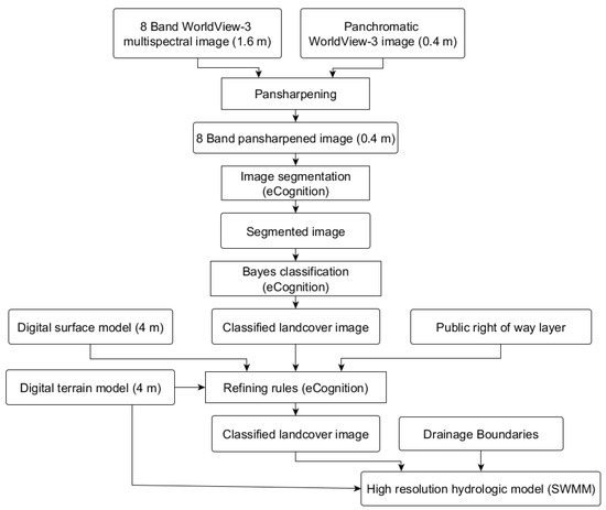
Figure 1.
Urban land cover classification and hydrologic model parameterization workflow.
2.2. Study Area
The majority of the 170 km2 Qing watershed rests within the Beijing City boundary (Figure 2) where it slopes from a maximum of 390 m a.s.l. in the Fragrant Hills area in Haidan district to a low of approximately 15 m a.s.l. where the Qing joins the Beiyun River in Chaoyang district in the East. The average annual rainfall is 525 mm and distribution throughout the year is uneven with over 80% of the precipitation occurring during the rainy season (June to September). The most highly urbanized upper portion of the Qing catchment (133 km2) was chosen as a study area. This part of the catchment contains within it many of Beijing’s research institutes and university campuses as well as the Olympic Park and several large residential areas.
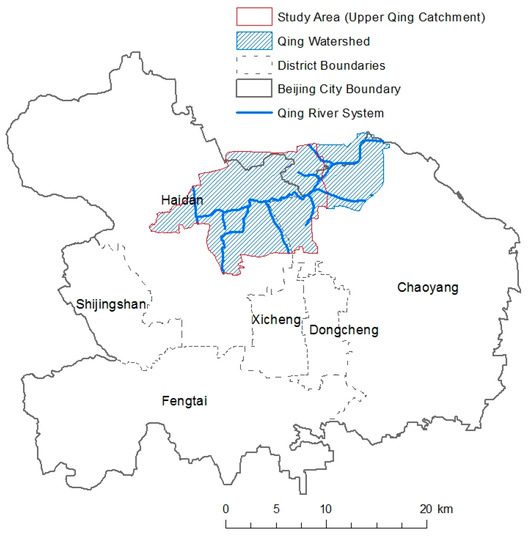
Figure 2.
Location of Upper Qing Catchment study area in Beijing, China.
2.3. Landcover Classification
2.3.1. Data and Software
Panchromatic and 8 band multispectral imagery from the WorldView-3 satellite (DigitalGlobe, Inc., Westminster, CO, USA) and 4 m resolution digital surface model (DSM) and digital terrain model (DTM) were acquired in September of 2017. To achieve an improved resolution, the multispectral bands (1.6 m resolution) of the WorldView-3 image were pansharpened [20] using the panchromatic band (0.4 m), yielding an image containing eight spectral bands with 0.4 m resolution. All segmentation and classification processes were performed using eCognition Developer 9 (Trimble Inc., Sunnyvale, CA, USA), a software package specialized in GEOBIA.
2.3.2. Segmentation
The process of segmentation aims to group neighboring pixels into objects at multiple scale levels, where the grouped pixels are relatively homogeneous in terms of the pixel values of the spectral bands [15]. The multiresolution segmentation algorithm [21] was applied to the image in eCognition. This algorithm performs segmentation of the image based on both spectral and geometric properties and has been shown to be highly successful when compared to other segmentation algorithms in the GEOBIA framework [22].
One study [23] focused on an overlapping study area in Beijing using the same imagery type and software as the current study, thus the multiresolution segmentation parameters found to be effective in that study were taken as guidance for parameter selection in the current study. The following parameters were assigned for multiresolution segmentation: scale value of 50, color weight of 0.9, shape weight of 0.1, compactness of 0.5, and smoothness of 0.5. Changing the value of any of these parameters effectively changes the shape and size of the generated objects. For the segmentation process, equal weight was set for each of the eight spectral bands of the WorldView-3 imagery (i.e., coastal blue, blue, green, yellow, red, red edge, and 2 NIR (near infrared) bands; NIR1 and NIR2).
2.3.3. Automated Land Cover Classification
Objects produced during segmentation can be classified using a rule-based procedure incorporating expert knowledge [24] or using machine learning algorithms based on training samples [23,25]. The approach taken in this study may be considered a combination of the two approaches as it begins with a machine learning algorithm for initial classification then proceeds to make classification refinements to improve accuracy using a set of refining rules.
There are several hundred spectral and spatial object features that can potentially be chosen as training parameters for classification. While the use of many training parameters may improve classification accuracy, the addition of each comes at a computational cost. In Qian et al. [23], a large number of object features frequently used for classification in previous studies were tested and several were determined to be optimal in terms of classification accuracy for the study area in Beijing. These were adopted in the current study and are summarized in Table 1.

Table 1.
Object features used for initial segmentation and classification.
The “Classifier” algorithm in eCognition applies machine learning functions in a two-step process: first a classifier is trained using the classified objects of the domain (i.e., the study area), as training samples. In the second step, the trained classifier is applied to the domain classifying the image objects according to the trained parameters. In Qian et al. [23] it was observed that of four image classifiers tested, the support vector machine (SVM) and Bayes classifier were most accurate, however Bayes was found to be more robust as it was not sensitive to time-consuming and potentially subjective setting of tuning parameters. The Bayes classifier, based on Bayesian statistics, is considered to be a parametric classifier as it groups pixel values based on a probability distribution, as opposed to non-parametric classifiers such as SVM or nearest neighbor which are based on deterministic theories and perform independent of the distribution of image values [26]. In Qian et al. [23], it was also observed that the use of more than 125 training samples per class provided minimal increases in classification accuracy. Consequently, the present study proceeded with use of the Bayes classifier and 125 training samples per class for classification of the segmented image.
Six land cover classes (including buildings, roads, paved pedestrian or parking area (PPPA), grass, trees and water) were chosen in this study based on their distinctness in terms of runoff characteristics as well as their relevance for the potential implementation of various LID infrastructure. The 125 objects chosen as training samples for each class were distributed across the study area. While a portion of the study area was traversed on foot to verify the correct class of some training samples, the majority (>95%) of training samples were assigned classes based on identification directly from the pansharpened image, assuming that a human operator can correctly identify the class.
2.3.4. Classification Refining Rules
As the initial classification based on the Bayes classifier alone had several common misclassifications, five refining rules were added to the eCognition ruleset following the initial application of the Bayes classifier (Table 2). First, Rule 1 was added to better differentiate between “grass” and “tree” objects. This rule was based on a comparison of the histograms for all object features (i.e., those listed in Table 1) of all grass and tree training samples. It was found that the standard deviation of the NIR band was the object feature with the least histogram overlap between the two classes, so a threshold value was set to separate the two classes.
Table 2.
Refining rules applied after Bayes classifier.
Shadows of buildings falling on adjacent impervious areas tended to have similar spectral properties to water, however these areas were typically much smaller in area and located immediately next to building objects. Therefore in Rule 2, all small (<25,000 pixel) objects classified as “water” were reclassified into a temporary class named “shadow”. In the second part of Rule 2, a histogram comparison was again used to set a threshold value for the object features which had the least overlap (i.e., red band and NDWI mean value), to reclassify additional water objects as shadow.
Due to similarity in spectral signatures many impervious surfaces were misclassified; for example, roads were incorrectly classified as PPPA and vice versa. To improve these classifications, in Rule 3 the impervious cover (i.e., objects classified as roads, PPPA, buildings or shadow) within the public right of way (i.e., the negative space in the land parcels boundaries data set available via Beijing City Lab [27]) were assumed to be roads. In Rule 4, impervious areas outside of the public right of way were assumed to be PPPA. Finally, in Rule 5 the difference between mean DTM (Digital Terrain Model) and mean DSM (Digital Surface Model) of the objects was used to separate buildings from surfaces with similar spectral signatures (i.e., PPPA). Adjacent objects of the same class were then merged. The interconnected roads polygons which ended up being very large due to the interconnected nature of roads were broken into smaller polygons of no longer than 500 m in length, to avoid the issue of all runoff from one large road subcatchment draining to a single outlet in the hydrologic model. The processing of the developed eCognition ruleset including segmentation, classification and classification refinement took approximately 5 h to run for the whole study area on a desktop with a 3.4 GHz i7 processor and 32 GB RAM.
2.3.5. Accuracy Assessment
After classification, the two output land cover maps (i.e., before and after application of refining rules) were tested against reference data to evaluate their accuracy. The Confusion matrix and Kappa statistics were calculated in eCognition. Reference data consisted of 100 objects for each of the six classes. Again, as with the training samples, the true class of the majority of reference objects was based on human interpretation of the pansharpened imagery, with only a small portion (<5%) being verified on the ground.
2.4. Hydrologic Model Setup
The current paper focuses primarily on land cover classification methods rather than hydrologic model development. A complete description of the SWMM model development, calibration and validation is provided in Randall et al. [28]. In short, the objects generated in the current study during the segmentation process were each assumed to represent a small subcatchment homogenous in terms of land cover. Each of these subcatchments drained to the nearest point of the hydraulic network located within the larger drainage area (Figure 3). Roads, buildings, and PPPA subcatchments were assumed to be 100% impervious (i.e., no infiltration can occur), while subcatchments classified as grass or trees were assigned to be 100% pervious (i.e., infiltration can occur over the whole area of the subcatchment). The open channel and subsurface hydraulics were inferred from the DTM with the assumption that stormwater mains are designed for a two year return period and run parallel to the primary roads. The developed model was calibrated and validated based on a range of rainfall events from 10 to 207 mm, yielding the hydrologic parameters shown in Table 3 [28].
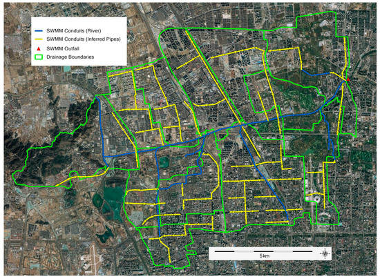
Figure 3.
Subsurface and open channel hydraulics represented in SWMM model.
Table 3.
SWMM model hydrologic parameters.
2.5. Sponge City Scenarios
In this study, the “Baseline” scenario assumed that no LID infrastructure has been implemented. The “High LID” scenario assumed that 60% of building areas are converted to green roofs, 70% of road or PPPA are converted to permeable pavement and 10% of grass or tree areas are converted to rain gardens. These values are based on the land conversion rates in China’s code for design of stormwater management [29] and the Sponge City Guidelines [1]. The “Mid LID” and “Low LID” scenarios assumed conversion rates equal to half and one quarter of the rates assumed in the High LID scenario, respectively. The parameters assigned to each LID type in the SWMM model (Table 4) were chosen in line with the Technical Guide for Sponge Cities Construction [1], other Sponge City studies in China [7,8,9] as well as guidance in the SWMM reference manual [30], which also contains detailed definitions of each model parameter.
Table 4.
Low Impact Development (LID) SWMM parameters applied.
2.6. Modelling of Design Events
While LID design has traditionally been aimed at capturing and treating events of return periods less than two years, engineers and planners are also typically required to evaluate these systems considering larger, less frequent events [31,32]. Therefore, in this study the volume reductions provided by varying levels of LID infrastructure for a range of design storms were evaluated to supplement the continuous modelling based on historic rainfall performed in Randall et al. [28]. The 3, 5, 10, 20, 50 and 100 year return period storms applied to the model were developed by the Beijing Urban Planning and Design Institute [33]. These storms are 24 h events characterized by a minor peak in the morning, and the majority of the rain occurring in the evening during a major peak lasting a few hours.
3. Results and Discussion
3.1. Landcover Classification
The segmentation of the WorldView-3 imagery yielded nearly 86,000 objects, each of which was then classified as belonging to one of the six land cover classes (Table 5). These segmentation and classification results were subsequently used for delineation and parameterization of the subcatchments in the hydrologic model. Segmented and classified images are shown alongside the original pansharpened Worldview-3 image for a magnified sample area (Figure 4). In general the segmentation parameters adopted from Qian et al. [23] were found to generate appropriately sized segments for the current application. Initial segmentation trials (i.e., those not following Qian et al. [23]) were found to often generate objects which were smaller than desired for the current application, e.g., individual cars on roads were delineated as separate objects.
Table 5.
Summary of segmentation/classification results.
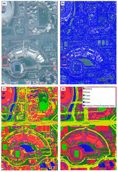
Figure 4.
Magnification of an example area (140 ha) within the Olympic Park shown as: WorldView-3 Pansharpened Image (0.4 m) (a) Segmented Image (b) Bayes Classified Image (c), and Bayes Classified Image (after refining rules) (d).
Classification results for the whole study area (Figure 5) showed that impervious areas (i.e., buildings, PPPA, roads) and green areas (i.e., trees, grass) account for approximately 52% and 46% of land cover, respectively. The trees class was the largest, covering nearly a third of the study area. The total tree area is likely slightly overestimated considering that tree canopy may extend beyond the pervious area where the trees are planted in some cases. Green areas are scattered throughout the whole study area, however are much more concentrated in the areas of Fragrant Hills and Old Summer Palace in the west and the Olympic Park in the east (Figure 5).
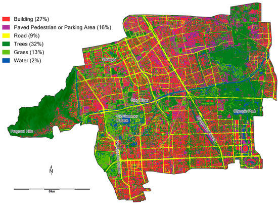
Figure 5.
Upper Qing Catchment study area, Beijing (133 km2) with land cover classified using Bayes classifier followed by application of refining rules.
3.2. Classification Accuracy Assessment
The Confusion matrices for classification based on the Bayes classifier alone (Table 6) and the Bayes classifier with the refining rules (Table 7) quantify the accuracies of each approach. In the matrices, “overall accuracy” refers to how many of the reference sites were classified correctly relative to the total number of reference sites. Producer’s accuracy represents how often real features on the ground are correct on the classified map, while the user’s accuracy represents how often the class on the map will actually be present on the ground. The Kappa coefficient evaluates how well the classification performed, where a value of 0 indicates that the classification is equivalent to random classification, and a value close to 1 indicates that the classification is significantly better than random.
Table 6.
Confusion Matrix for classification using Bayesian classifier.
Table 7.
Confusion Matrix for classification using Bayesian classifier followed by refining rules.
The accuracy assessment indicated that when the refining rules were applied to the initial classification produced by the Bayes classifier, both the overall accuracy and the Kappa coefficient increased significantly, from 63% to 76%, and from 0.56 to 0.72, respectively. While there is no broad consensus on an overall accuracy that should be achieved for an application like the current one, a commonly referenced standard in the broader remote sensing literature suggests 85 to 90% [34]. The current study fell short of this target both before and after application of the refining rules. The required Kappa coefficient also depends greatly on the specific application, however the values achieved in the current study fall in the category of “substantial agreement” (i.e., from 0.61 to 0.80) based on the Kappa statistics groupings suggested by Landis and Koch [35].
The greatest improvement after the refining rules were applied was the user’s accuracies for the Roads and PPPA classes (i.e., from 45 to 81% and from 14 to 68%, respectively). The spectral signatures of these mostly pavement covered areas tended to be very similar, and therefore the supplementary topological data (i.e., the right of way layer) was required to more consistently differentiate between them. Another observed significant improvement was the producer’s accuracy for the buildings class, which increased from 48 to 92% due to the refining rule which considered the difference in values between the DSM and DTM. The accuracy assessment results have thus demonstrated the value of supplementary data sets when performing GEOBIA classification of VHR imagery in urban areas with a high concentration of impervious surfaces with similar spectral signatures. Classification of green areas (i.e., trees and grass) was also improved with the refining rules. Using the Bayes classifier alone, tree objects were frequently (29 times out 100) incorrectly classified as grass. The refining rule attempted to improve this through the use of a threshold value of the standard deviation of the NIR band (Section 2.3.3), resulting in an increase in the producer’s accuracy of trees from 67 to 80%.
However, even after the refining rules were applied not all of the individual accuracy metrics were significantly improved, and a few had values somewhat lower than before the refining rules were applied. The buildings class user’s accuracy, for example, lowered after application of the refining rules. Most objects that the Bayes classifier alone classified as buildings were in fact buildings, however there were also many (52 out of 100) building objects not classified as buildings. This high user’s accuracy combined with low producer’s accuracy represents an error of omission (i.e., not enough pixels have been classified as a given class). It should be noted that after application of the refining rules the Building class producer’s accuracy increased much more than the user’s accuracies decreased, considered an acceptable tradeoff that contributed to a higher overall accuracy. After application of the refining rules, 92 of the 100 building objects were correctly identified as Buildings.
The Kappa coefficients and overall accuracy obtained for the classification based on the Bayes classifier alone (i.e., 0.56 and 63%, respectively), were not nearly as high as the 0.96 and 96% obtained by Qian et al. [23], which also used 125 training samples and the Bayes classifier for GEOBIA in an overlapping study area in Beijing. The accuracies found in the current study were also lower than the mean overall accuracy of 83.6% given for Worldview data based classification studies in general [19]. There are likely a number of explanations for these discrepancies. Firstly, the classes used by Qian et al. [23] did not differentiate between trees and grass or between the various types of impervious cover and these are by far the most common misclassifications in the current study. If the six classes chosen for this study were reduced to three as in Qian et al. [23] (i.e., water, green areas and impervious areas), the overall accuracy would exceed 90% and be in line with the results found in that study. In general, the more specific and numerous the classes are, the more difficult it is to correctly assign objects to the correct class. This is confirmed by the review by Ma et al. [19], where it was found that there is a negative correlation between the overall classification accuracy and the number of classes defined.
Secondly, the fact that the current study area was relatively large with likely higher variation within each of the land cover types may account for the somewhat lower accuracies. Applying GEOBIA to a smaller area may yield higher accuracies as urban features tend to be more similar to nearby features than they are to features in other parts of the city. For example, most of the residential buildings in one neighborhood of a city may have similar spectral characteristics because of the construction materials and methods used when that area was developed.
Fortunately, the most common misclassifications were not highly impactful in terms of overall stormwater runoff properties. For example, misclassifying roads as PPPA and vice versa does not significantly impact the results of the hydrological modelling for this particular study as both classes were assumed to have the same runoff properties and rates of conversion to permeable pavement in the LID scenarios. Misclassification of roads into the building class, for example, would be more impactful to the hydrologic modelling results because each of these class’ respective LIDs (i.e., permeable pavement and green roofs) perform differently.
3.3. Hydrologic Modelling
The land cover classification obtained from the GEOBIA procedure presented above aided in the development of a hydrologic model that returns realistic results [28] and can be run reasonably efficiently (i.e., 1 h per scenario, per event, using a 3.4 GHz i7 processor and 32 GB RAM). Runoff hydrographs as computed by the SWMM model (Figure 6) show that runoff peak flows and volumes in the Qing River decrease as the level of LID implementation increases for all return periods, as is expected. Also as expected, the computed runoff volume reductions relative to the Baseline scenario runoff volume (Table 8) increases with an increasing level of LID implementation and decreases with an increase in return period of the event. However, the volume reduction for the Low LID scenario did not change significantly with return period, i.e., 62 and 61% of runoff volume was retained for the 3 and 100 year events, respectively. In the High LID scenario the volume reduction changes somewhat more with return period (i.e., 82 and 77% for the 3 and 100 year storms, respectively). This is likely because the extent of LID coverage limits the amount of runoff that can be captured for lower return period events, whereas the storage capacity of the LID is more of a limiting factor for higher return period storms (i.e., many LID are overflowing during large storms). There is therefore a need to know where the rainfall can be captured within the city in addition to the volume that can be captured at that location. Use of the detailed land cover data allows for these spatial considerations in hydrologic modelling. Although there is likely some potential for controlled conveyance of water to LID offsite, the general principles of LID call for onsite capture, and this is what was represented in the SWMM model. That is, runoff can only drain to LID within the subcatchment, or in the case of rain gardens, also from the adjacent impervious Road, Building or PPPA subcatchments.

Figure 6.
Event hydrographs at model outfall for Baseline and LID scenarios under 3 (a), 5 (b), 10 (c), 20 (d), 50 (e), and 100 (f) year 24 h Beijing design storms.
Table 8.
Modelled runoff volume reductions relative to the Baseline scenario under varying 24 h return period events and levels of LID implementation.
While the 77% volume reduction of the 100 year event for the High LID scenario represents a substantial decrease in runoff, it should be noted that this scenario represents an ambitious level of implementation that will require a large portion of the study area to be retrofitted from its current state. Nevertheless, the results indicate that it is physically possible for a significant portion of a large event to be captured using LID infrastructure built to common specifications and considering the limitations of the urban landscape.
It should be noted that the SWMM model currently does not include representation of overland flow routes. Runoff that cannot be accommodated within the sewer system simply ponds on top of the model node until there is capacity available in the storm sewer system. For this reason, peak flows of very large events may not be modelled accurately if significant overland flow would occur in reality. However, even for the larger storms the total volume reductions provided by LID systems are likely accurate as the storage within the LID will be filled before overland flow occurs in the model. To more accurately represent peak flow reduction, lag times, or surface ponding depths for high return period storms, the current 1D model would need to be coupled with an additional 1D or 2D hydraulic model to simulate surface flow paths. If the current model were at some point to be enhanced with such representation of overland flow, the detailed land cover map developed in this study will provide further value in terms of identifying the overland flow obstacles (i.e., buildings) and assigning roughness values to the various urban surfaces.
4. Study Limitations and Future Research
There are various areas within the study catchment that do not fit well into one of the six land cover classes chosen in this study. For example, outdoor sports facilities do not necessarily behave hydrologically as many grassed park areas do, however they were typically classified as grass areas. Also, it was observed that, in a few cases, areas consisting mainly of bare soil were classified as “PPPA”. It is likely that many of the bare soil areas in the study area are under construction and will in the future be some other type of primarily impervious surface (either building or PPPA). These areas that do not exactly fit into one of the chosen classes make up a relatively small portion of the total study area and therefore the addition of more classes was considered to add complexity for minimal benefit.
The approach taken in the current study was based on approaches described in previous studies for the choice of segmentation settings, object features and training classifiers and therefore did not include rigorous testing of the many variables within each of these, all of which will impact results. While ideally an analysis on the sensitivity of all these variables’ impact on classification accuracy would be evaluated, the rather large size of the study area made such evaluation challenging.
The GEOBIA approach has provided a sufficiently accurate output of classes that are relevant to hydrologic modeling. The approach taken here was relatively simple and it is possible that a higher accuracy could be achieved using the same satellite imagery. Indeed, there are many classification techniques that may yield an improved result that have not been explored here, for example the inclusion of texture based object features [36]. While initial testing during this study included some basic texture features as segmentation/classification parameters, they were found to slow down the computation time significantly due to the size of the study area. Given that many hydrologic modelling studies may not have the expertise or resources available to fully optimize the classification of large urban areas, an approach similar to the one taken here may be most feasible in many cases.
The land cover classification approach described can be applied to different catchments in Beijing, as well as in other cities after adjustment. To apply the method elsewhere, the Bayes classifier would need to be retrained with local sample objects for each land cover class. The refining rules can also be applied after the threshold values have been adjusted. For example, the threshold value of the NIR standard deviation used to differentiate grass and trees objects in Rule 1 (Table 2), is likely to vary considerably between cities or even between data sets collected from the same city during different seasons. Additional refining rules may need to be developed to address common misclassifications specific to another urban environment.
The initial use of the hydrologic model in this study considers only possible hydrologic impacts of Sponge City implementation in the context of the current urban landscape under current design storms and average summer temperatures. In other work [28], continuous modelling based on historical rainfall and temperature demonstrated use of the same model to evaluate potential Sponge City impacts of more frequent rain events on the long term water balance. Still, there remains considerations that could be explored using the model, particularly related to possible future changes. Beijing is a rapidly developing city and the built up area is continuing to grow and change which will have impacts on runoff as well as temperatures. Furthermore, climate change is expected to increase urban temperatures as well as design storm volumes and intensities. Accounting for these factors is likely to yield different volume reduction rates than those presented here. Future work with the model may therefore include investigation of the future hydrologic impacts of these factors individually and in combination.
5. Conclusions
While GEOBIA has evolved from related methods developed over the past several decades, this approach for image classification has been described as a new paradigm in the field of remote sensing [18]. Yet, exploration of GEOBIA’s potential as a tool for use in the field of stormwater management specifically is currently limited. In this study it was demonstrated that application of GEOBIA to WorldView-3 satellite imagery is capable of efficiently and accurately identifying the extent of impervious and pervious cover at a very high resolution (i.e., 0.4 m) for a large (i.e., >100 km2) urban study area. However, for further differentiation of land cover into more specific classes (e.g., trees vs. grass, and multiple types of impervious surfaces), the use of spectral data alone was not as satisfactory. The classification results were not found to be as accurate as those reported in other studies which used smaller areas and/or fewer classes, likely due to the large size and corresponding high variability of the study area features in combination with the relatively high number of land cover classes.
For applications such as the current one, which benefit from accurate differentiation between the various impervious surfaces (i.e., buildings, roads, parking lots), the advantage of incorporating additional data sources and applying a set of refining rules was made clear by comparison of the classification accuracy before and after a set of refining rules. The data required for this additional classification refinement can range from free (e.g., land parcel delineations from Beijing City Lab) to several thousand euros (>10,000 RMB) per 100 km2 (e.g., moderately high resolution DSM/DTM data).
The approach taken in this study is based on the techniques described in previous studies; however it has applied these techniques to a significantly larger study area and thus demonstrated the feasibility of producing acceptably accurate GEOBIA classification of large urban catchments, a current gap existing in the literature. This study has also served as an example of GEOBIA classification with the specific end goal of generating input to urban hydrologic models, an application which is lacking in the GEOBIA literature.
The hydrologic model based on the GEOBIA land cover classification was able to run numerous design storm scenarios efficiently despite the many thousands of drainage areas delineated. With the computer processing power available to most modelers, there seems little downside to leveraging the high level of surface detail that can be derived from satellite imagery for parameterization of urban hydrologic models when the relevant GIS data are not already available. The majority of computational demand from models like SWMM tends to come from the hydraulic calculations (e.g., flows in pipes) rather than the rainfall runoff computations which can rapidly be performed for thousands of subcatchments. Results from the hydrologic model indicated that a significant portion of the runoff volume from large storms could be retained within the study catchment using LID. While these results are encouraging, it should be noted that even the Low LID scenario explored here represents a significant portion of the urban landscape being retrofitted and it will take considerable effort to achieve such a high level of implementation across the whole catchment.
Author Contributions
M.R. and R.F., Y.Z. and M.B.J. conceived and designed the experiments; M.R. performed the experiments/modelling; M.R. analyzed the data; M.R. wrote the paper with input from R.F., Y.Z. and M.B.J.
Funding
This research and the APC were funded by the Sino-Danish Center.
Acknowledgments
We would like to thank the Sino-Danish Center (SDC) and the Natural Sciences and Engineering Research Council of Canada (NSERC) for their generous PhD scholarship support. We would also like to thank software and data providers including Computational Hydraulics International, DHI-GRAS and Trimble for providing reduced cost or free software, data and guidance for the research. Also, thank you to the input we have received along the way from many colleagues, especially those at the Beijing Water Science and Technology Institute.
Conflicts of Interest
The authors declare no conflict of interest.
References
- Ministry of Housing and Urban-Rural Development. Technical Guide for Sponge Cities-Construction of Low Impact Development; Architecture & Building Press: Beijing, China, 2014. [Google Scholar]
- Fletcher, T.D.; Shuster, W.; Hunt, W.F.; Ashley, R.; Butler, D.; Arthur, S.; Trowsdale, S.; Barraud, S.; Semadeni-Davies, A.; Bertrand-Krajewski, J.-L.; et al. SUDS, LID, BMPs, WSUD and more—The evolution and application of terminology surrounding urban drainage. Urban Water J. 2015, 12, 525–542. [Google Scholar] [CrossRef]
- Cheng, M.; Qin, H.; He, K.; Xu, H. Can floor-area-ratio incentive promote low impact development in a highly urbanized area?—A case study in Changzhou City, China. Front. Environ. Sci. Eng. 2018, 12, 8. [Google Scholar] [CrossRef]
- Gao, J.; Wang, R.; Huang, J.; Liu, M. Application of BMP to urban runoff control using SUSTAIN model: Case study in an industrial area. Ecol. Model. 2015, 318, 177–183. [Google Scholar] [CrossRef]
- Jia, H.; Lu, Y.; Yu, S.L.; Chen, Y. Planning of LID–BMPs for urban runoff control: The case of Beijing Olympic Village. Sep. Purif. Technol. 2012, 84, 112–119. [Google Scholar] [CrossRef]
- Li, H.; Ding, L.; Ren, M.; Li, C.; Wang, H. Sponge City Construction in China: A Survey of the Challenges and Opportunities. Water 2017, 9, 594. [Google Scholar] [CrossRef]
- Chang, X.; Xu, Z.; Zhao, G.; Du, L. Urban rainfall-runoff simulations and assessment of low impact development facilities using SWMM model-A case study of Qinghe catchment in Beijing. J. Hydroelectr. Eng. 2016, 35, 84–93. [Google Scholar]
- Kong, F.; Ban, Y.; Yin, H.; James, P.; Dronova, I. Modeling stormwater management at the city district level in response to changes in land use and low impact development. Environ. Model. Softw. 2017, 95, 132–142. [Google Scholar] [CrossRef]
- Mei, C.; Liu, J.; Wang, H.; Yang, Z.; Ding, X.; Shao, W. Integrated assessments of green infrastructure for flood mitigation to support robust decision-making for sponge city construction in an urbanized watershed. Sci. Total Environ. 2018, 639, 1394–1407. [Google Scholar] [CrossRef] [PubMed]
- Krebs, G.; Kokkonen, T.; Valtanen, M.; Koivusalo, H.; Setälä, H. A high resolution application of a stormwater management model (SWMM) using genetic parameter optimization. Urban Water J. 2013, 10, 394–410. [Google Scholar] [CrossRef]
- Krebs, G.; Kokkonen, T.; Valtanen, M.; Setälä, H.; Koivusalo, H. Spatial resolution considerations for urban hydrological modelling. J. Hydrol. 2014, 512, 482–497. [Google Scholar] [CrossRef]
- Khin, M.M.L.; Shaker, A.; Joksimovic, D.; Yan, W.Y. The use of WorldView-2 satellite imagery to model urban drainage system with low impact development (LID) Techniques. Geocarto Int. 2016, 31, 92–108. [Google Scholar] [CrossRef]
- Berezowski, T.; Chormański, J.; Batelaan, O.; Canters, F.; Van de Voorde, T. Impact of remotely sensed land-cover proportions on urban runoff prediction. Int. J. Appl. Earth Obs. Geoinf. 2012, 16, 54–65. [Google Scholar] [CrossRef]
- Dams, J.; Dujardin, J.; Reggers, R.; Bashir, I.; Canters, F.; Batelaan, O. Mapping impervious surface change from remote sensing for hydrological modeling. J. Hydrol. 2013, 485, 84–95. [Google Scholar] [CrossRef]
- Blaschke, T. Object based image analysis for remote sensing. ISPRS J. Photogramm. Remote Sens. 2010, 65, 2–16. [Google Scholar] [CrossRef]
- Cleve, C.; Kelly, M.; Kearns, F.R.; Moritz, M. Classification of the wildland–urban interface: A comparison of pixel- and object-based classifications using high-resolution aerial photography. Comput. Environ. Urban Syst. 2008, 32, 317–326. [Google Scholar] [CrossRef]
- Myint, S.W.; Gober, P.; Brazel, A.; Grossman-Clarke, S.; Weng, Q. Per-pixel vs. object-based classification of urban land cover extraction using high spatial resolution imagery. Remote Sens. Environ. 2011, 115, 1145–1161. [Google Scholar] [CrossRef]
- Blaschke, T.; Hay, G.J.; Kelly, M.; Lang, S.; Hofmann, P.; Addink, E.; Queiroz Feitosa, R.; van der Meer, F.; van der Werff, H.; van Coillie, F.; et al. Geographic Object-Based Image Analysis—Towards a new paradigm. ISPRS J. Photogramm. Remote Sens. 2014, 87, 180–191. [Google Scholar] [CrossRef]
- Ma, L.; Li, M.; Ma, X.; Cheng, L.; Du, P.; Liu, Y. A review of supervised object-based land-cover image classification. ISPRS J. Photogramm. Remote Sens. 2017, 130, 277–293. [Google Scholar] [CrossRef]
- Li, H.; Jing, L.; Tang, Y. Assessment of Pansharpening Methods Applied to WorldView-2 Imagery Fusion. Sensors 2017, 17, 89. [Google Scholar] [CrossRef]
- Baatz, M.; Schäpe, A. Multiresolution Segmentation: An optimization approach for high quality multi-scale image segmentation. In Angewandte Geographische Informationsverarbeitung XII; Strobl, J., Blaschke, T., Griesebner, G., Eds.; Wichmann: Heidelberg, Germany, 2000; pp. 12–23. [Google Scholar]
- Neubert, M.; Herold, H.; Meinel, G. Assessing image segmentation quality—Concepts, methods and application. In Object-Based Image Analysis–Spatial Concepts for Knowledge-Driven Remote Sensing Applications; Blaschke, T., Hay, G., Lang, S., Eds.; Lecture Notes in Geoinformation & Cartography 18; Springer: Berlin, Germany, 2008; pp. 769–784. [Google Scholar]
- Qian, Y.; Zhou, W.; Yan, J.; Li, W.; Han, L. Comparing Machine Learning Classifiers for Object-Based Land Cover Classification Using Very High Resolution Imagery. Remote Sens. 2014, 7, 153–168. [Google Scholar] [CrossRef]
- Zhou, W.; Troy, A. An object-oriented approach for analysing and characterizing urban landscape at the parcel level. Int. J. Remote Sens. 2008, 29, 3119–3135. [Google Scholar] [CrossRef]
- Maxwell, A.E.; Warner, T.A.; Strager, M.P.; Conley, J.F.; Sharp, A.L. Assessing machine-learning algorithms and image- and lidar-derived variables for GEOBIA classification of mining and mine reclamation. Int. J. Remote Sens. 2015, 36, 954–978. [Google Scholar] [CrossRef]
- Phiri, D.; Morgenroth, J. Developments in Landsat Land Cover Classification Methods: A Review. Remote Sens. 2017, 9, 967. [Google Scholar] [CrossRef]
- Long, Y.; Wu, K.; Mao, Q. Simulating urban expansion in the parcel level for all Chinese cities. arXiv 2014, arXiv:1402.3718. Available online: https://arxiv.org/abs/1402.3718 (accessed on 10 March 2018).
- Randall, M.; Sun, F.; Zhang, Y.; Bergen Jensen, M. Evaluating Sponge City volume capture ratio at the catchment scale using SWMM. J. Environ. Manag. 2019, in press. [Google Scholar]
- BIAD (Beijing Institute of Architectural Design); Beijing General Municipal Engineering Design and Research Institute; Beijing Institute for Water Science and Technology. Code for Design of Stormwater Management and Harvesting Engineering; BIAD (Beijing Institute of Architectural Design); Beijing General Municipal Engineering Design and Research Institute; Beijing Institute for Water Science and Technology: Beijing, China, 2013. Available online: http://www.bjwater.gov.cn/bjwater/resource/cms/2016/12/old_image/P020150805747401290775.pdf (accessed on 22 January 2018).
- Rossman, L.; Huber, W. Storm Water Management Model Reference Manual Volume I—Hydrology (Revised); U.S. Environmental Protection Agency: Cincinnati, OH, USA, 2016.
- Coffman, L. Low-Impact Development Design Strategies: An Integrated Design Approach; Department of Environmental Resources, Programs and Planning Division: Prince George’s County, MD, USA, 1999. [Google Scholar]
- Rosa, D.; Clausen, J.; Dietz, M. Calibration and Verification of SWMM for Low Impact Development. J. Am. Water Resour. Assoc. (JAWRA) 2015, 51, 746–757. [Google Scholar] [CrossRef]
- Beijing Urban Planning and Design Institute. Standard of Rainstorm Runoff Calculation for Urban Storm Drainage System Planning and Design; Beijing Municipal Planning and Land Resources Administration Commission of Beijing Quality and Technical Supervision: Beijing, China, 2016.
- Anderson, J.R.; Hardy, E.E.; Roach, J.T.; Witmer, R.E. A Land Use and Land Cover Classification System for Use with Remote Sensor Data; United States Geological Survey: Arlington, VA, USA, 1976.
- Landis, J.R.; Koch, G.G. The Measurement of Observer Agreement for Categorical Data. Biometrics 1977, 33, 159–174. [Google Scholar] [CrossRef]
- Kim, M.; Madden, M.; Warner, T.A. Forest Type Mapping using Object-specific Texture Measures from Multispectral Ikonos Imagery. Photogramm. Eng. Remote Sens. 2009, 75, 819–829. [Google Scholar] [CrossRef]
© 2019 by the authors. Licensee MDPI, Basel, Switzerland. This article is an open access article distributed under the terms and conditions of the Creative Commons Attribution (CC BY) license (http://creativecommons.org/licenses/by/4.0/).