Article

Spatial Variabilities of Runoff Erosion and Different Underlying Surfaces in the Xihe River Basin

1
College of Urban and Environmental Sciences, Northwest University, Xi’an 710127, China
2
College of Surveying and Geo-Informatics, North China University of Water Resources and Electric Power, Zhengzhou 450045, China
3
Yellow River Institute of Hydraulic Research, Zhengzhou 450003, China
4
School of Civil Engineering, Shandong University, Jinan 250061, China
*
Authors to whom correspondence should be addressed.
Water 2019, 11(2), 352; https://doi.org/10.3390/w11020352
Submission received: 14 December 2018 / Revised: 14 February 2019 / Accepted: 15 February 2019 / Published: 19 February 2019

Abstract

:
Runoff erosion capacity has significant effects on the spatial distribution of soil erosion and soil losses. But few studies have been conducted to evaluate these effects in the Loess Plateau. In this study, an adjusted SWAT model was used to simulate the hydrological process of the Xihe River basin from 1993 to 2012. The spatial variabilities between runoff erosion capacity and underlying surface factors were analyzed by combining spatial gradient analysis and GWR (Geographically Weighted Regression) analysis. The results show that the spatial distribution of runoff erosion capacity in the studying area has the following characteristics: strong in the north, weak in the south, strong in the west, and weak in the east. Topographic factors are the dominant factors of runoff erosion in the upper reaches of the basin. Runoff erosion capacity becomes stronger with the increase of altitude and gradient. In the middle reaches area, the land with low vegetation coverage, as well as arable land, show strong runoff erosion ability. In the downstream areas, the runoff erosion capacity is weak because of better underlying surface conditions. Compared with topographic and vegetation factors, soil factors have less impact on runoff erosion. The red clay and mountain soil in this region have stronger runoff erosion capacities compared with other types of soils, with average runoff modulus of 1.79 × 10⁻³ m3/s·km2 and 1.68 × 10⁻³ m3/s·km2, respectively, and runoff erosion power of 0.48 × 10⁻⁴ m4/s·km2 and 0.34 × 10⁻⁴ m4/s·km2, respectively. The runoff erosion capacity of the alluvial soil is weak, with an average runoff modulus of 0.96 × 10⁻³ m3/s·km2 and average erosion power of 0.198 × 10⁻⁴ m4/s·km2. This study illustrates the spatial distribution characteristics and influencing factors of hydraulic erosion in the Xihe River Basin from the perspective of energy. It contributes to the purposeful utilization of water and soil resources in the Xihe River Basin and provides a theoretical support for controlling the soil erosion in the Hilly-gully region of the Loess Plateau.

1. Introduction

Soil erosion has been defined as the processes of detachment and transport of soil materials by erosive agents [1]. These processes are largely determined by overland flow, and the runoff generated by the effective rainfall that does not infiltrate [2] carries a large amount of sediment which deposits in the river, raises the riverbed, aggravates the flooding, and brings great potential dangers to the lives and property of the people in the middle and lower reaches is the main driving factor of soil erosion. It is imperative to quantify relationships between the runoff erosion and Different Underlying Surfaces for better understanding of erosion processes [3], and to further provide a theoretical basis for soil erosion control and ecological restoration [4,5].
With the increasing knowledge acquired in the study of soil erosion, current focuses of research on soil erosion [6,7,8] include clarifying the mechanism of surface coverage and underlying topography on erosion, putting forward reasonable control methods, and understanding the spatial pattern of hydraulic erosion and its influencing factors in hilly-gully regions. The research on the relationship between soil erosion and different underlying surface conditions mainly has the following two aspects. On the one hand, the characteristics of soil erosion are assessed based on empirical models [9,10,11,12,13,14,15,16,17,18]. For example, Thomas et al. [19] calculated the long-term average annual soil loss and sediment yield by using a combination of the Revised Universal Soil Loss Equation (RUSLE) and the sediment delivery ratio (SDR) models in the Southern Western Ghats, India. Mehra et al. [17] used the universal soil loss equation (USLE) model to identify soil resource management zones and develop site-specific soil management plan in the Mewat district in the semiarid regions of Haryana, India. Mondal [16] assessed and compared the results obtained from three soil erosion models using a GIS platform in a part of Narmada River and drew a conclusion that the RUSLE model is the most reliable. On the other hand, the effect of different factors on erosion and sediment yield is analyzed based on physical and hydrological models [20,21,22,23,24,25]. For example, Jeziorska [26] estimated that the optimal timespan is half a year for the TOPMODEL to perform at its best in the Central Sudetes (SW Poland). Sheng et al. [27] investigated the hydrological impacts of changes in land use and precipitation by using a MIKESHE model in the Chaohe watershed, China. Res et al. [28] used a Geoweep model to estimate sediment yield and runoff from Keklik watershed, Turkey.
However, results from empirical calculations lack consideration of physical mechanisms and neglect the spatial reasons for runoff generation. In physical hydrological models, the spatial difference between different types of land is often generalized, leading to unclear spatial variabilities between erosion and vegetation condition as well as between erosion and soil material. To address the shortcomings of using empirical models and other physical models, the Soil and Water Assessment Tool (SWAT) has been developed. SWAT is a semi-distributed physical hydrological model. It has been widely used in runoff and sediment studies under different scenarios [29,30,31,32], with a practical advantage for studying the Hilly-gully region with complex underlying surface conditions [33,34,35]. For example, Shivhare et al. [36] used ArcGIS and ArcSWAT to identify the erosion prone areas for effective planning and management of groundwater resources in Ganga watershed, India. Yesuf et al. [37] optimized the parameters of the SWAT using monthly observed sediment yield data at a monitoring site in Maybar experimental watershed, Ethiopia. Duru et al. [38] used the SWAT to generate a soil erosion map and concluded that significant portions of urbanized and highly cultivated areas in the vicinity of stream channels are particularly vulnerable to soil erosion.
In this study, the SWAT model was used to simulate the runoff of the Xihe River Basin. The runoff modulus and runoff erosion power were used as indexes to evaluate the runoff erosion capacity. The spatial distribution relationships between runoff erosion capacity and different surface coverage, soil infiltration capacity, and topographic factors were analyzed to reveal the effects of spatial distribution on soil erosion. This study aimed at providing a theoretical support for the protection of soil and water in the Xihe River Basin.

2. Materials and Methods
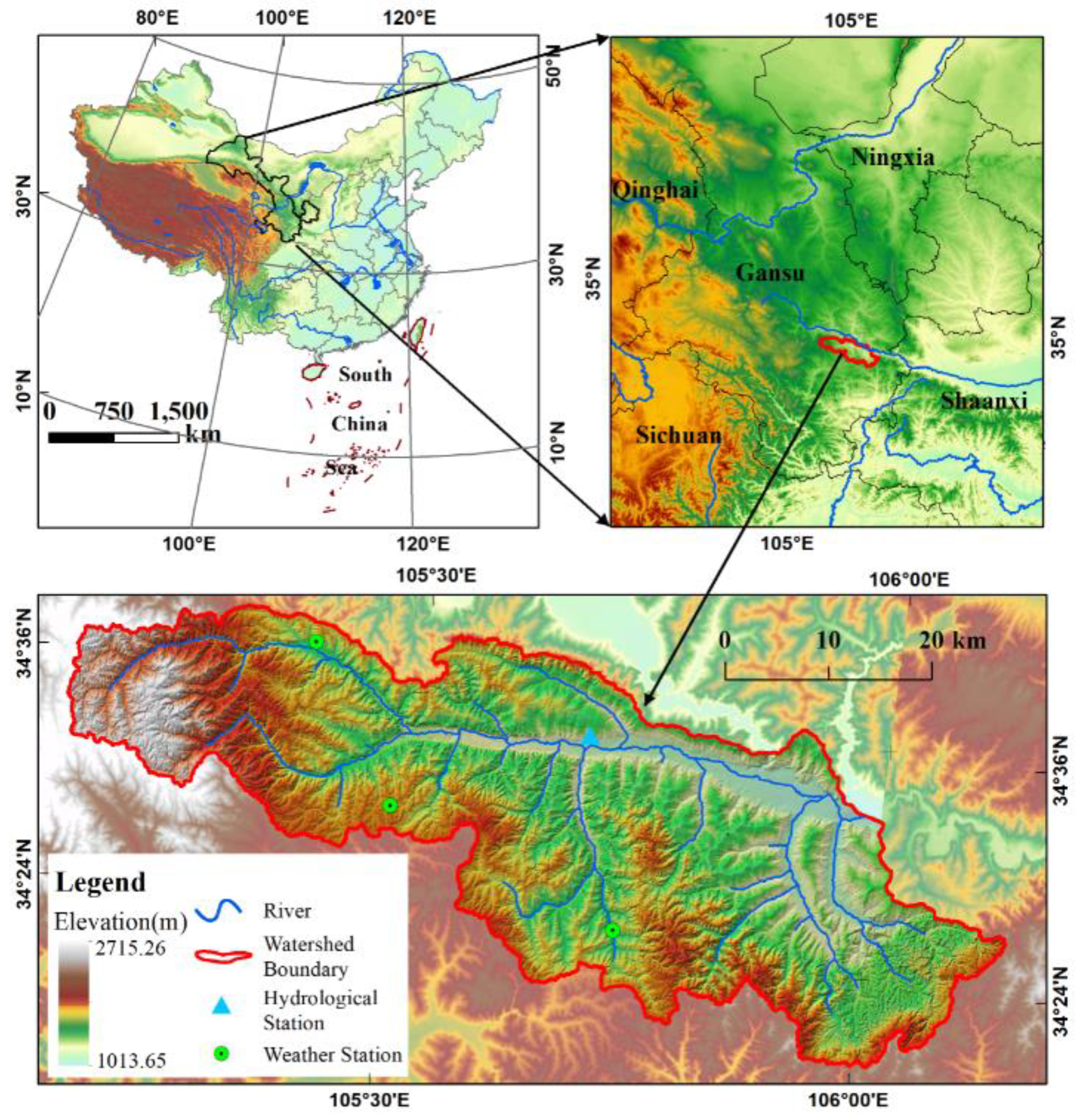
2.1. Study Area

Xihe River is a first-class tributary of the upper and middle reaches of Weihe River. It is located at the northern foothill of Qinling Mountains and the southern edge of Longxi Loess Plateau. It rises at the eastern foot of Jingdongliang Mountain in Longtai Mountain, Tianshui City, Gansu Province, and joins the Weihe River at the Beidaobu gateway in Maiji District. The whole length of the river is 85 km, the area of the basin is 1267 km2, the altitude is 1013~2715 m, and the geographical range is between 34°20′ N ~ 34°38′ N and 105°07′ E ~ 106°00′ E. It belongs to the third sub-region of the Loess Hilly-gully region. The terrain of the basin is fragmented and complex with crisscrossing ravines and gullies, and the terrain is high in the northwest and low in the southeast. The overview of the Xihe River Basin is shown in Figure 1. The Xihe River Basin belongs to a sub-humid climate in the warm temperate zone. Its annual average temperature is 10.5 °C and annual precipitation is 558.9 mm. The precipitation varies greatly between years, distributes unevenly during the year, and takes place mainly in July–September. The spatial distribution of precipitation is as follows: the south is significantly larger than the north with no obvious difference between the east and the west. The soil types are complex and the spatial distribution of soil types in the Xihe River Basin is shown in Figure 2. The main types are loessial soil (accounting for 35.9%), cinnamon soil (accounting for 21.5%), and brown soil (accounting for 19.1%). The loessial soil is mainly distributed in gully, which is 1100–1500 m above sea level. The soil is thick, crisp, and easily be water-eroded in case of heavy rain. The cinnamon soil is mainly distributed in the area of 1500–2100 m above sea level in Qinling Mountain. The brown soil is mainly distributed in the southwest with an altitude of 1500 m–2500 m. The main vegetation is deciduous broad-leaved forest in warm temperate zone, which is in the transition zone from forest grassland to grassland. The natural shrub grassland is mainly distributed in the loess beam and the lower hills, with a coverage rate of 33.05%. This basin has severe soil erosion because of long-term unreasonable reclamation.

2.2. Data Sources

The data used in the SWAT model include: (1) Digital Elevation Model (DEM): the 30 m resolution DEM is generated by vectorization of 1:50,000 paper topographic map and interpolation with the software ANUDEM (The Australian National University-DEM). (2) Land use maps: a land use map with 30 m resolution was generated with an interpretation of Landsat7 remote sensing images on 30 June 2001. (3) Soil data: the 1:1 million scale HWSD (Harmonized World Soil Database) database was constructed by FAO (Food and Agriculture Organization of the United Nations) and the International Institute for Applied Systems Analysis. (4) Hydrometeorological data: daily hydrological precipitation data of Tianshui Hydrological Station and daily precipitation data of Guanzizhen Station, Huangjizhai Station and Xujiadian Station were collected from Volume 7 of Hydrological Data of the Yellow River Basin (1990–2012), and daily meteorological monitoring data from the Tianshui Station of China Meteorological Data Network including average temperature, daily maximum temperature, daily minimum temperature, average relative humidity, average wind speed, and sunshine time. Data used for result analysis include: (1) remote sensing data of vegetation: monthly composite data of MODIS (2000–2012)—MODND1M 500 m NDVI (Normalized Vegetation Index) provided by Geospatial Data Cloud. (2) Soil seepage stabilization data: the steady seepage rate was measured by a double-loop infiltration method in the field from May to October 2008. The 30 m resolution raster data were generated by Kriging interpolation.

2.3. SWAT Model

The SWAT model is a model developed by the Agricultural Research Center of the United States Department of Agriculture. It is mainly used to simulate and predict the impact of land use and various land managements on watershed water quality and quantity [39]. The model has a strong physical mechanism and can simulate various hydrophysical and chemical processes using spatial information provided by GIS and RS [40,41]. The SWAT differentiates several sub-basins under the support of DEM, and then differentiates the sub-basins into several hydrological response units (HRUs) according to land use, soil type, and topographic gradient. The response-unit runoff is calculated by a conceptual lumped model on each HRU, and the total runoff of the basin is calculated by a confluence calculation. The model has been widely used by scientists in hydrological assessment, environmental change, sensitivity analysis, and other fields [42,43,44,45]. With this model, Chinese researchers have achieved good results in the Weihe River Basin [46,47], Heihe River Basin [48,49,50], Wujiang River Basin [23], Yanhe River Basin [51,52,53], Dongjiang River Basin [54], etc.

2.3.1. Model Construction

The projection coordinate system required by the model was Xian_1980_Albers. The central longitude was 105.5° E, the first standard latitude was 34.6° N, and the second standard latitude was 34.3° N. Soil database and meteorological data database were established according to the requirements of model database construction. The minimum catchment area of the river was set to 1900 ha (19 km2) based on repeated debugging, and the thresholds of land use, soil type, and slope were set to 15%, 10%, and 15%, respectively. A total of 51 sub-basins and 545 HRUs were obtained.
To improve the simulation accuracy of the model and obtain a good initial state, the preheating period of the model was set to 1990–1992, the parameter calibration period was set to 1993–2009, and the validation period was set to 2010–2012.

2.3.2. Sensitivity Analysis and Parameter Calibration

In this study, a sensitivity analysis was conducted using an LH-OAT (Latin-Hypercube and One-factor-At-a-time sampling) method for obtaining the main parameters and controlling the number of calibration parameters. Relevant runoff sensitivity parameters were obtained to make the model work efficiently. Taking into consideration that the SCS (Soil Conservation Service) runoff curve value (CN2) has high sensitivity with a heavy impact on runoff simulations, and different land use types have different CN2 values, these values were calibrated according to different land use types. 15 parameters with high sensitivity were selected to calibrate by using a SUFI-2 algorithm of SWAT-CUP software based on the monthly runoff data of Tianshui Hydrological Station from 1993 to 2009. The results are shown in Table 1.

2.4. Runoff Erosion Ability Index

Taking into consideration that the intensity of soil erosion in the research area could not be effectively represented by runoff data, runoff modulus and runoff erosion power were selected as the indexes of runoff erosion ability to explore the spatial variabilities between runoff erosion ability and different underlying surface conditions.
Runoff modulus eliminates the influence from the size of a basin and better indicates the runoff characteristics of a basin. Runoff erosion power reflects the combined effect of the rainfall process and the conditions of the underlying surface, which can better reflect the role of hydraulic erosion [51,55,56] and the combined effect of different underlying surface conditions in the watershed on erosion and sediment yielding [52]. Related expressions are summarized in Table 2.

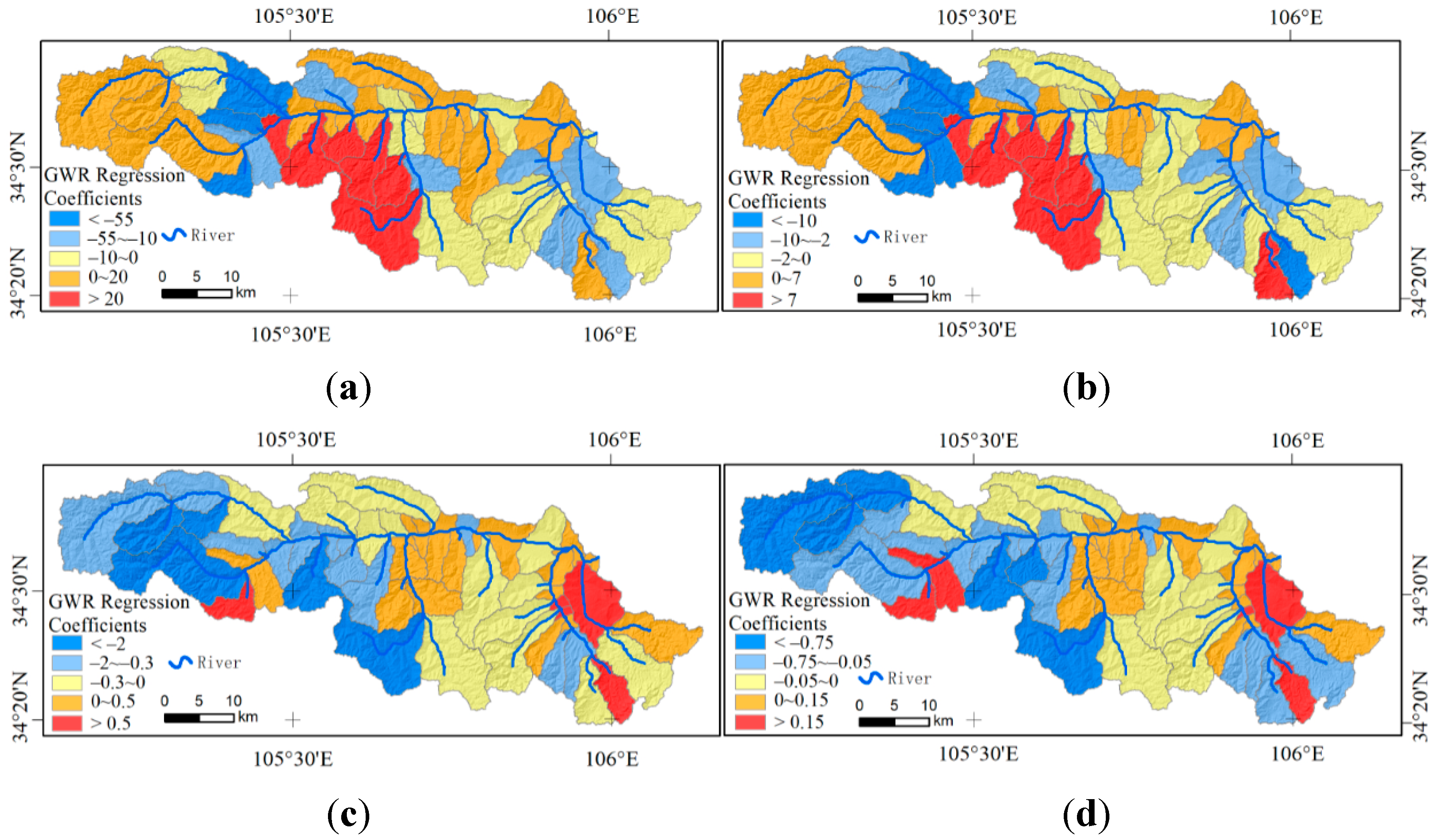
2.5. Geographically Weighted Regression Model

Geographically Weighted Regression (GWR) is a method to study the quantitative relationship between two or more variables with spatial or regional distribution characteristics by using the principle of regression [57]. The GWR model is an extension of the traditional regression model. In this model, independent equations are constructed for each element in the data set. It is used to merge dependent variables and explanatory variables that fall within the bandwidth of each target element to evaluate the spatial variation. The expression of GWR model is as follows:
y i =   β 0 ( u i , v i ) + k = 1 n β k ( u i , v i ) x i k + ε i
In the equation, (ui, vi) refer to the coordinate of the ith sample; β0(ui, vi) and βk(ui, vi) refer to the intercept and slope, respectively, of the GWR model at the regression point i; k is the number of independent variables; yi, xik, and ε i are the dependent variable, independent variables, and random error, respectively, at the regression point i.

3. Results

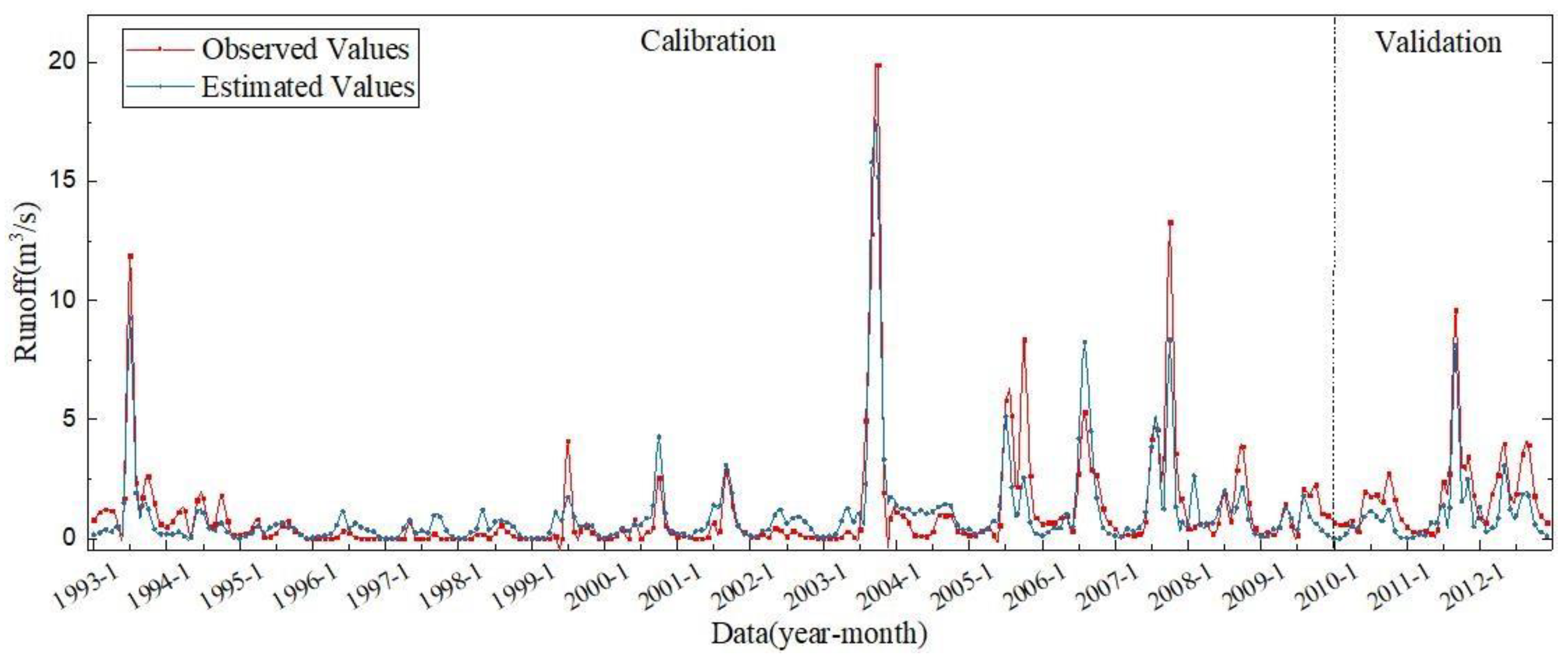
3.1. The SWAT Model Runoff Calibration and Verification

The monthly runoff simulation values of Tianshui Station in the calibration period (1993–2009) and verification period (2010–2012) were obtained after several parameter adjustments. A comparison between the observed runoff values and the simulated runoff values of Tianshui Station (1993–2012) is shown in Figure 3.
It can be seen from Figure 3 that the simulated monthly runoff values agree well with the observed monthly runoff values. However, the simulation of flood peaks is insufficient, and the simulated values are lower than the observed ones. To evaluate the accuracy of the simulations, the deterministic coefficient R2 and Nash-Sutcliffe efficiency coefficient (ENS) were used to evaluate the applicability of the simulated results. When the the deterministic coefficient R2 approaches 1, the simulated results became more accurate. ENS indicated the degree of deviation between the simulated and observed values. When the closer the ENS approach 1, the closer the simulated results were to the observed values. The ENS was calculated using the equation as shown below:
E N S = 1 i = 1 n ( Q o Q s ) 2 i = 1 n ( Q o Q ¯ ) 2
In the equation, Q o is the observed value, Q s is the simulated value, and Q ¯ is the average observed value. Generally, when ENS is greater than or equal to 0.6, the simulation results are good; when ENS is greater than or equal to 0.7, the simulation results are very good [58].
The accuracy of the simulated calibration results was evaluated using 35 peak flow results occurring during the study period: in the calibration period, R2 is 0.81 and ENS is 0.81; in the validation period, R2 is 0.88 and ENS is 0.65; in the peak simulation period (as shown in Figure 4), R2 is 0.77 and ENS is 0.65. These results indicate that the simulation performance of the model for the flood peak period of the river basin is not as accurate as the flat-water period, but the overall simulation results are accurate during the study period. These values indicate that the model has a strong applicability to the Xihe River Basin and well reflects the hydrological conditions of the basin. It provides a data basis for further exploring the spatial variabilities between the runoff erosion capacity and underlying surface conditions in the basin.

3.2. Spatial Pattern of Runoff Erosion Capacity

The monthly runoff data of 51 sub-basins in the Xihe River Basin from 1993 to 2012 were collected based on the simulation results using the SWAT model. The annual runoff modulus and runoff erosion power of each sub-basin could be obtained according to equations (1) and (2) in Table 2. To reflect the general rule of spatial distribution of runoff erosion capacity of the sub-basins, the 20-year average calculations for the sub-basins were used to obtain the spatial distribution of annual average runoff modulus and runoff erosion power in the Xihe River Basin from 1993 to 2012, as shown in Figure 5.
Figure 5 shows that the spatial distribution of runoff modulus and runoff erosion power are similar in the Xihe River Basin. Runoff erosion was more likely to occur in the northern part of the basin than in the southern part. The runoff erosion capacity of most areas in the western part of the basin was stronger than that of the eastern part, but there was also a tributary in the eastern part of the basin with strong runoff erosion capacity. The area with strong runoff erosion capacity (0.17 < Eyear < 0.35) accounted for 29% of the whole basin area, and the area with very strong erosion capacity (Eyear > 0.35) accounted for 13% of the whole basin area.

3.3. Gradient Analysis of Runoff Erosion Capacity and Topographic Factors

Based on the elevation of the river basin ranging from 1013 to 2715 m, 545 HRUs were grouped based on elevation gradients as < 1500 m, 1500~2000 m, 2000~2500 m, and > 2500 m; and grouped based on slope gradients as <5°, 5~15°, 15~25°, and >25°. The Mean and Standard Deviation (SD) of runoff modulus and runoff erosion power based on the hydrological response unit were calculated and shown in Figure 6.
Figure 6a shows that the runoff modulus increases with the increase of elevation and slope. When the elevation reached 2000 m, the runoff modulus generally tended to be stable and the dispersion degree did not change much, but it decreased in the high elevation and low slope areas (elevation 2500 m and slope < 5°), which accounted for about 0.1% of the total watershed area. When the elevation was below 2000 m, the dispersion degree of runoff modulus increased with the increase of slope under the same terrain gradient. When the elevation was between 1500 and 2000 m, the dispersion degree of runoff modulus was the strongest. Figure 6b shows that the runoff erosion power increases with the increase of altitude at the same slope gradient. When the elevation was lower than 2000 m, the dispersion of runoff erosion power between different slope gradients was notable, and the dispersion degree increased with the increase of slope gradients. When the altitude was in a range from 1500 m to 2000 m, the runoff erosion power varied regularly with the slope gradient, and the dispersion degree was the highest.

3.4. Relationship between Runoff Erosion Capacity and Vegetation Factors

3.4.1. Vegetation Coverage in the Basin

The average value of NDVI in the basin from 2000 to 2012 was calculated to determine the vegetation coverage in the study period of the Xihe River Basin. The results shown in Figure 7 indicate that the vegetation coverage in the West and Southeast regions, which account for 32.6% of the basin area, was good (NDVI > 0.5). The northern region (about 25% of the basin area) had less vegetation coverage than the southern region.

3.4.2. Spatial Correlation with Vegetation Index

In this study, the local correlation between runoff modulus and runoff erosion power of 51 sub-basins and multi-year average NDVI was analyzed by using the Geographically Weighted Regression (GWR) model. The spatial relationship between runoff erosion capacity and surface vegetation was clarified to ensure the accuracy and credibility of the analysis results. An optimal bandwidth of 3.45 km was determined by using the local correlation coefficient R2 of the GWR model as a reference. The spatial variation between runoff erosion capacity and surface vegetation coverage in the Xihe River Basin was obtained as shown in Figure 8a,b.
The results show that the spatial correlation between runoff modulus (Figure 8a), runoff erosion power (Figure 8b), and multi-year annual average NDVI was similar to each other. The difference between areas with positive correlation and areas with negative correlation of runoff modulus and annual NDVI was not significant. The positive correlation area accounted for about 50.9% of the total area of the basin. It was mainly located in the southwest and central regions of the basin. The positive correlation was stronger in the central region than in the southwest region. The correlation between runoff erosion power and annual average NDVI was mainly negative, with an area accounting for approximately 56.6% of the whole basin area. The negative correlation area was mainly located in the eastern and northern parts of the basin. Since most of the land in the central region was used as agricultural land with weak ability of water storage and soil conservation, the runoff erosion capability showed a positive correlation in this region.

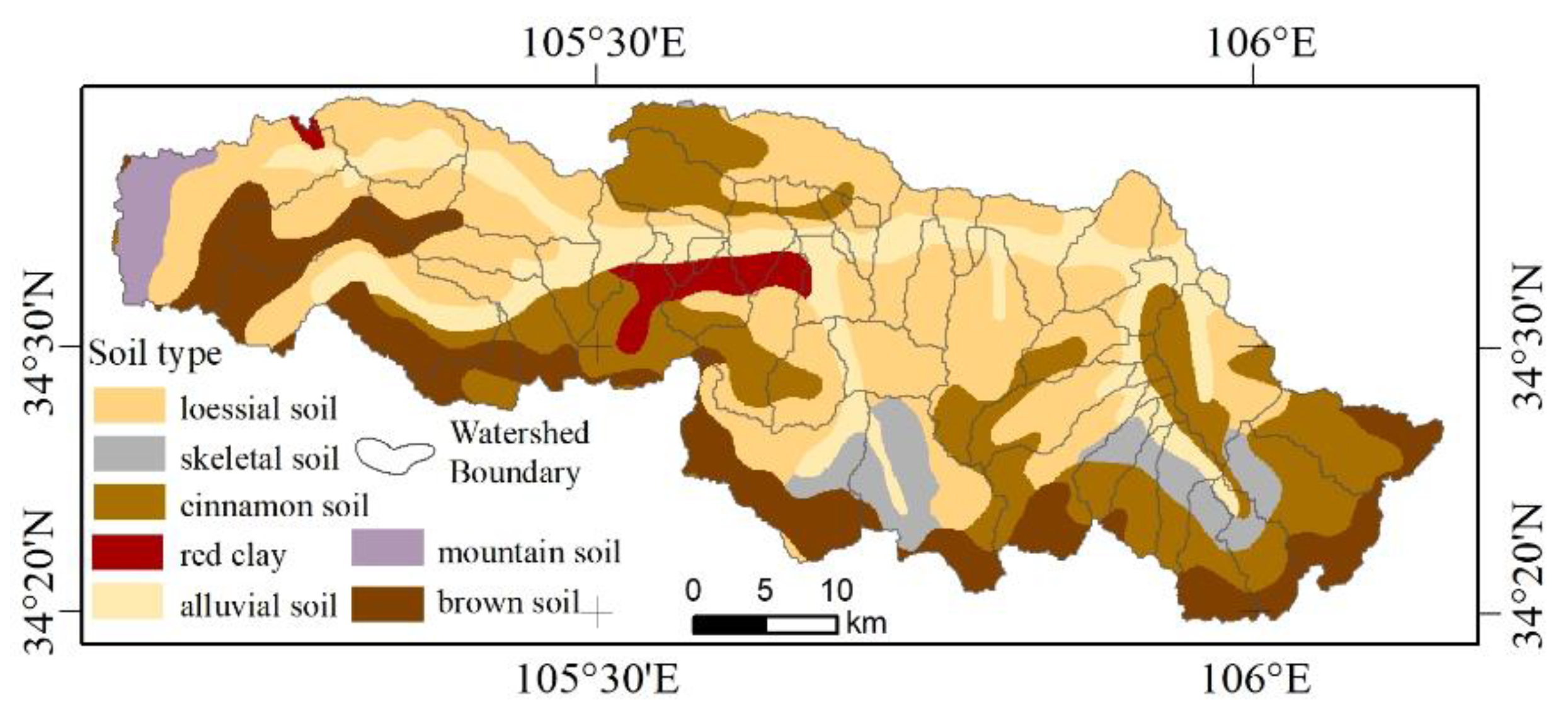
3.5. Spatial Variability of Runoff Erosion Capacity and Soil Factors

Soil infiltration is an important aspect in the process of mutual transformation of precipitation, surface water, soil water, groundwater, and plant water. Soil infiltration rate can indirectly indicate the soil erosion resistance. The spatial distribution characteristics of soil types in this basin are shown in Figure 2. In this study, the local correlation between runoff modulus, runoff erosion power, and stable soil infiltration rate of 51 sub-basins was analyzed by using the GWR model with an optimal bandwidth of 3.7 km, as shown in Figure 8c,d.
The results in the Figure 8c,d show that the spatial distribution of positive and negative correlation between runoff modulus, runoff erosion power, and stable soil infiltration rate was consistent. The correlation was mainly negative, accounting for 73.8% of the total area, and was mainly in the upper and middle reaches of the basin. The negative correlation was the strongest in the southwest of the basin. The outlet location of the basin showed a relatively strong positive correlation. The correlation between runoff erosion power and steady soil infiltration rate was weak based on numerical analyses of regression coefficients using the GWR model. Compared with topographic and vegetation factors, the influence of steady soil infiltration rate on runoff erosion capacity was weaker.
Based on results shown in Figure 2 and Figure 5, taking the runoff modulus and runoff erosion power of different soil types into consideration, the runoff erosion capacities of different soil types in the Xihe River basin were obtained as shown in Table 3.
Based on Table 3, the red clay and mountain soil in this region have strong runoff erosion capacities, with average runoff modulus of 1.790 × 10⁻³ m3/s·km2 and 1.680 × 10⁻³ m3/s·km2, respectively, and average runoff erosion power of 0.480 × 10⁻⁴ m4/s·km2 and 0.34 × 10⁻⁴ m4/s·km2. The runoff erosion capacity of the alluvial soil is weak, with an average runoff modulus of 0.960 × 10⁻³ m3/s·km2 and average erosion power of 0.198 × 10⁻⁴ m4/s·km2.

4. Discussion

In this study, parameters with great influences on the runoff simulation were determined by multiple calibrations, so that the SWAT model could fully exert its advantages to achieve better simulation results. The SWAT model is different from commonly used empirical soil erosion models such as the RUSLE model, which has simple input requirements and can conveniently calculate the soil erosion modulus of a small watershed, but cannot be applied to accurately simulate soil erosion at different regions. While the SWAT model is a watershed-based model, the RUSLE model which is mainly used as a hillslope-based model even though in both models’ similar components are taken into consideration. Based on the input of long-term sequence data, the watershed is divided into response units according to the information of land use type, soil type, and terrain slope by using the SWAT mode. The SWAT model uses measured runoff data to calibrate the simulated results and achieve consistence with real situations. Because of its accuracy, the SWAT model has been widely used to achieve convincing results. In the large-scale watershed, Ajaaj et al. [59] used SWAT model evaluated the accuracy of four widely used satellite and gauged-based precipitation products in the poorly gauged Tigris River basin, Middle East. Tang et al. [60] used the SWAT model to evaluate the suitability of five widely used global high-resolution precipitation products in Lancang river basin, China. In the middle-scale watershed, Lyu et al. [61] simulated the hydrological cycle and analyzed the influence of climate variability and land use change on green water resources from 1995 to 2015 in the Xihe River Basin, China. Nunes et al. [62] got a successful result and determined the watershed’s use efficiency by using the meteorological data which from 2000 to 2010 in the Capim River watershed, Brazil. In the small-scale watershed, Qiao et al. [63] developed a model for heavy metal migration simulation based on the SWAT in Huanjiang watershed, China. Though the SWAT model has been widely used in many fields, it still has a complex calibration process. The calibration can be facilitated by calculating the K factor, C factor, and P factor in the RUSLE model.
In this paper, the spatial pattern of runoff erosion capacity and its relationship with spatial variabilities of different underlying surface factors in the Xihe River Basin have been studied. The simulated results agree with the real observations. The runoff modulus and runoff erosion power were used to effectively characterize the runoff erosion capacity of the region. The GWR model was used to quantitatively analyze the spatial correlation between runoff erosion indexes, vegetation coverage, and soil factors. This study contributes to the purposeful utilization of water and soil resources in the Xihe River Basin and provides a theoretical support for controlling the soil erosion in the Hilly-gully region of the Loess Plateau.

5. Conclusions

In this study, the runoff process in Xihe River basin was simulated by using the SWAT model based on the hydrological observation data from 1990 to 2012. The runoff modulus and runoff erosion power, which are two indicators for the runoff erosion capacity, were calculated from the simulation results. The runoff erosion was discussed in combination with topography, vegetation, and underlying surface factors. The spatial variabilities characteristics are as follows:
  • The SWAT model has a good applicability in the arid Xihe River Basin in the Loess Plateau. The spatial pattern of runoff erosion capacity in the Xihe River Basin has the following characteristics: strong in the north, weak in the south, strong in the west, and weak in the east. Approximately 13% of the total area of the basin is prone to runoff erosion.
  • The runoff modulus increases with the increase of elevation and slope. Surface vegetation coverage (NDVI) is closely related to the runoff erosion capacity. However, not all areas with high vegetation coverage have weak runoff erosion capacity, indicating that merely increasing vegetation coverage cannot improve soil erosion in the areas where runoff erosion capacity is positively correlated with NDVI. The correlation between runoff erosion capacity and stable soil infiltration rate is mainly negative (accounting for 73.8% of total area). However, compared with other factors, the influence of soil factor on runoff erosion capacity is smaller. The red clay and mountain soil in this region have strong runoff erosion capacities, while the alluvial soil has a weak runoff erosion capacity.
  • In the upper reaches of the Xihe River, topographic factors such as elevation and slope gradient are the dominant factors affecting the runoff erosion. In the northern part of the basin, the runoff erosion is strong due to the low coverage of vegetation. In the middle reaches of the basin, the land is mainly used for cultivation, strong runoff is caused by the combination of topographic fluctuations and land use. Since runoff erosion is strong in this region, farming shall be replaced with forest and grass learning from adjacent sub-basins to reduce the soil erosion. In the downstream area, the runoff erosion is weak due to lower altitude, small topographic fluctuation, good vegetation coverage, and good soil infiltration.

Author Contributions

N.W. designed and carried out the experiments and wrote the manuscript. Z.Y. and X.L. collected the data for experiments and provided significant suggestions on the methodology and structure of the manuscript. W.L. and M.M. gave a lot helps to solve the questions during the experiments. All authors contributed to the discussions and approved the final manuscript.

Funding

This research was funded by National key research priorities program of China-Variation mechanism and trend prediction of water and sediment in the Yellow River Basin (2016YFC0402402) and The Open Fund from Key Laboratory of Soil and Water Loss Process and Control on the Loess Plateau of the Ministry of Water Resources-Simulation of Soil and Water Loss Process in Hill and Gully Region of the Loess Plateau Based on GIS (2016005).

Acknowledgments

Daily hydrological precipitation data were collected from Yellow River Institute of Hydraulic Research and Xi’an University of Technology.

Conflicts of Interest

The authors declare no conflict of interest.

References

  1. Ellison, W.D. Soil erosion studies—Part I. Agric. Eng. 1947, 28, 145–146. [Google Scholar]
  2. Keesstra, S.D.; Temme, A.; Schoorl, J.M.; Visser, S.M. Evaluating the hydrological component of the new catchment-scale sediment delivery model LAPSUS-D. Geomorphology 2014, 212, 97–107. [Google Scholar] [CrossRef]
  3. Rodrigo-Comino, J.; Davis, J.; Keesstra, S.D.; Cerda, A. Updated Measurements in Vineyards Improves Accuracy of Soil Erosion Rates. Agron. J. 2018, 110, 411–417. [Google Scholar] [CrossRef]
  4. Keesstra, S.; Mol, G.; de Leeuw, J.; Okx, J.; de Cleen, M.; Visser, S. Soil-related sustainable development goals: Four concepts to make land degradation neutrality and restoration work. Land 2018, 7, 133. [Google Scholar] [CrossRef]
  5. Keesstra, S.; Nunes, J.P.; Saco, P.; Parsons, T.; Poeppl, R.; Masselink, R.; Cerda, A. The way forward: Can connectivity be useful to design better measuring and modelling schemes for water and sediment dynamics? Sci. Total Environ. 2018, 644, 1557–1572. [Google Scholar] [CrossRef] [PubMed]
  6. Liu, S.; An, N.; Yin, Y.; Cheng, F.; Dong, S. Relationship between spatio-temporal dynamaics of soil and water loss and NDVI of the small basins in the middle reaches of Lancang River based on SWAT model. J. Soil Water Conserv. 2016, 30, 62–67. [Google Scholar]
  7. Sun, J.; Yu, D.; Shi, X.; Gu, Z.; Zhang, W.; Yang, H. Comparision of between LAI and VFC in relationship with siol erosion in the red soil hilly region of south China. Acta Pedol. Sin. 2010, 47, 1060–1066. [Google Scholar]
  8. Wang, G.; Zhang, C.; Liu, J.; Wei, J.; Xue, H.; Li, T. Analyses on the variation of vegetation coverage and water sediment reduction in the rich and coarse sediment area of the Yellow River basin. J. Sediment Res. 2006, 2, 10–16. [Google Scholar]
  9. Patovvary, S.; Sarma, A.K. GIS-Based Estimation of Soil Loss from Hilly Urban Area Incorporating Hill Cut Factor into RUSLE. Water Resour. Manag. 2018, 32, 1–13. [Google Scholar] [CrossRef]
  10. Qin, W.; Guo, Q.; Cao, W.; Yin, Z.; Yan, Q.; Shan, Z.; Zheng, F. A new RUSLE slope length factor and its application to soil erosion assessment in a Loess Plateau watershed. Soil Tillage Res. 2018, 182, 10–24. [Google Scholar] [CrossRef]
  11. Hu, G.; Song, H.; Shi, X.; Zhang, M.; Liu, X.; Zhang, X. Soil erosion characteristics based on RUSLE in the Wohushan Reservoir Watershed. Sci. Geogr. Sin. 2018, 38, 610–617. [Google Scholar]
  12. Li, D.; Yang, J.; Li, W.; Zhu, C. Evaluating the sensitivity of soil erosion in the Yili River valley based on GIS and USLE. Chin. J. Ecol. 2016, 35, 942–951. [Google Scholar]
  13. Liao, Y.; Zhuo, M.; Xie, J.; Wei, G.; Guo, T.; Xie, Z.; Li, D. Variations in vegetation cover factors and their influence on USLE and RUSLE. Acta Ecol. Sin. 2017, 37, 1987–1993. [Google Scholar]
  14. Peng, S.; Yang, K.; Hong, L.; Xv, Q.; Huang, Y. Spatio-temporal evolution analysis of soil erosion based on USLE model in Dianchi Basin. Trans. Chin. Soc. Agric. Eng. 2018, 34, 138–146. [Google Scholar]
  15. Thomas, J.; Joseph, S.; Thrivikramji, K.P. Assessment of soil erosion in a tropical mountain river basin of the southern Western Ghats, India using RUSLE and GIS. Geosci. Front. 2018, 9, 893–906. [Google Scholar] [CrossRef]
  16. Mondal, A.; Khare, D.; Kundu, S. A comparative study of soil erosion modelling by MMF, USLE and RUSLE. Geocarto Int. 2018, 33, 89–103. [Google Scholar] [CrossRef]
  17. Mehra, M.; Singh, C.K. Spatial analysis of soil resources in the Mewat district in the semiarid regions of Haryana, India. Environ. Dev. Sustain. 2018, 20, 661–680. [Google Scholar] [CrossRef]
  18. Bhowmik, M.; Das, N.; Das, C.; Ahmed, I.; Debnath, J. Bank material characteristics and its impact on river bank erosion, West Tripura district, Tripura, North-East India. Curr. Sci. 2018, 115, 1571–1576. [Google Scholar] [CrossRef]
  19. Thomas, J.; Joseph, S.; Thrivikramji, K.P. Assessment of soil erosion in a monsoon-dominated mountain river basin in India using RUSLE-SDR and AHP. Hydrol. Sci. J. 2018, 63, 542–560. [Google Scholar] [CrossRef]
  20. Guo, H.; Hu, Q.; Jiang, T. Annual and seasonal streamflow responses to climate and land-cover changes in the Poyang Lake basin, China. J. Hydrol. 2008, 355, 106–122. [Google Scholar] [CrossRef]
  21. Li, Z.; Liu, W.-Z.; Zhang, X.-C.; Zheng, F.-L. Impacts of land use change and climate variability on hydrology in an agricultural catchment on the Loess Plateau of China. J. Hydrol. 2009, 377, 35–42. [Google Scholar] [CrossRef]
  22. Feng, C.; Mao, D.; Zhou, H.; Cao, Y.; Hu, G. Impacts of climate and land use changes on runoff in the Lianshui basin. J. Glaciol. Geocryol. 2017, 39, 395–406. [Google Scholar]
  23. Hou, W.; Gao, J.; Dai, E.; Peng, T.; Wu, S.; Wang, H. The runoff generation simulation and its spatial variation analysisin Sanchahe basin as the south source of Wujiang. Acta Geogr. Sin. 2018, 73, 1268–1282. [Google Scholar]
  24. Li, S.; Wei, H.; Liu, Y.; Ma, W.; Gu, Y.; Peng, Y.; Li, C. Runoff prediction for Ningxia Qingshui River Basin under scenarios of climate and land use changes. Acta Ecol. Sin. 2017, 37, 1252–1260. [Google Scholar]
  25. Da Silva, V.D.R.; Silva, M.T.; De Souza, E.P. Influence of land use change on sediment yield: A case study of the sub-middle of the Sao Francisco River basin. Eng. Agric. 2016, 36, 1005–1015. [Google Scholar] [CrossRef]
  26. Jeziorska, J.; Niedzielski, T. Applicability of TOPMODEL in the mountainous catchments in the upper Nysa Kodzka river basin (SW Poland). Acta Geophys. 2018, 66, 203–222. [Google Scholar] [CrossRef]
  27. Wang, S.-P.; Zhang, Z.-Q.; Ge, S.; Strauss, P.; Guo, J.-T.; Yao, A.-K.; Tang, Y. Assessing Hydrological Impacts of Changes in Land Use and Precipitation in Chaohe Watershed Using MIKESHE Model. J. Ecol. Rural Environ. 2012, 28, 320–325. [Google Scholar]
  28. Reis, M.; Aladag, I.A.; Bolat, N.; Dutal, H. Using Geoweep model to determine sediment yield and runoff in the Keklik watershed in Kahramanmaras, Turkey. Sumar. List 2017, 141, 563–569. [Google Scholar]
  29. Xu, H.; Xu, C.-Y.; Saelthun, N.R.; Xu, Y.; Zhou, B.; Chen, H. Entropy theory based multi-criteria resampling of rain gauge networks for hydrological modelling—A case study of humid area in southern China. J. Hydrol. 2015, 525, 138–151. [Google Scholar] [CrossRef]
  30. Lv, L.; Peng, Q.; Guo, Y.; Liu, Y.; Jiang, Y. Runoff simulation of Dongjiang River Basin based on the soil and water assessment tool. J. Nat. Resour. 2014, 29, 1746–1757. [Google Scholar]
  31. Yuan, Y.; Zhnag, Z.; Meng, J. Impact of changes in land use and climate on the runoff in Liuxihe Watershed based on SWAT model. Chin. J. Appl. Ecol. 2015, 26, 989–998. [Google Scholar]
  32. Zhao, A.; Liu, X.; Zhu, X.; Pan, Y.; Li, Y. Spatiotemporal patterns of droughts based on SWAT model for the Weihe River Basin. Prog. Geogr. 2015, 34, 1156–1166. [Google Scholar]
  33. Hao, F.H.; Zhang, X.S.; Yang, Z.F. A distributed non-point source pollution model: Calibration and validation in the Yellow River basin. J. Environ. Sci. 2004, 16, 646–650. [Google Scholar]
  34. Xu, H.; Taylor, R.G.; Xu, Y. Quantifying uncertainty in the impacts of climate change on river discharge in sub-catchments of the Yangtze and Yellow River Basins, China. Hydrol. Earth Syst. Sci. 2011, 15, 333–344. [Google Scholar] [CrossRef] [Green Version]
  35. Zuo, D.; Xu, Z.; Yao, W.; Jin, S.; Xiao, P.; Ran, D. Assessing the effects of changes in land use and climate on runoff and sediment yields from a watershed in the Loess Plateau of China. Sci. Total Environ. 2016, 544, 238–250. [Google Scholar] [CrossRef] [PubMed]
  36. Shivhare, N.; Rahul, A.K.; Omar, P.J.; Chauhan, M.S.; Gaur, S.; Dikshit, P.K.S.; Dwivedi, S.B. Identification of critical soil erosion prone areas and prioritization of micro-watersheds using geoinformatics techniques. Ecol. Eng. 2018, 121, 26–34. [Google Scholar] [CrossRef]
  37. Yesuf, H.M.; Assen, M.; Alamirew, T.; Melesse, A.M. Modeling of sediment yield in Maybar gauged watershed using SWAT, northeast Ethiopia. Catena 2015, 127, 191–205. [Google Scholar] [CrossRef]
  38. Duru, U.; Arabi, M.; Wohl, E.E. Modeling stream flow and sediment yield using the SWAT model: A case study of Ankara River basin, Turkey. Phys. Geogr. 2018, 39, 264–289. [Google Scholar] [CrossRef]
  39. Wang, Z.; Liu, C.; Huang, Y. The theory of SWAT model and its application in Heihe Basin. Prog. Geogr. 2003, 22, 79–86. [Google Scholar]
  40. Chen, C.; Zhang, Y.; Xiang, Y.; Wang, L. Study on runoff responses to land use change in Ganjiang Basin. J. Nat. Resour. 2014, 29, 1758–1769. [Google Scholar]
  41. Zhang, D.; Zhang, W.; Zhu, L.; Zhu, Q. Improvement and application of SWAT—A physically based, distributed hydrological model. Sci. Geogr. Sin. 2005, 25, 434–440. [Google Scholar]
  42. Golden, H.E.; Sander, H.A.; Lane, C.R.; Zhao, C.; Price, K.; D’Amico, E.; Christensen, J.R. Relative effects of geographically isolated wetlands on streamflow: A watershed-scale analysis. Ecohydrology 2016, 9, 21–38. [Google Scholar] [CrossRef]
  43. Haregeweyn, N.; Tsunekawa, A.; Poesen, J.; Tsubo, M.; Meshesha, D.T.; Fenta, A.A.; Nyssen, J.; Adgo, E. Comprehensive assessment of soil erosion risk for better land use planning in river basins: Case study of the Upper Blue Nile River. Sci. Total Environ. 2017, 574, 95–108. [Google Scholar] [CrossRef] [PubMed] [Green Version]
  44. Muenich, R.L.; Kalcic, M.; Scavia, D. Evaluating the Impact of Legacy P and Agricultural Conservation Practices on Nutrient Loads from the Maumee River Watershed. Environ. Sci. Technol. 2016, 50, 8146–8154. [Google Scholar] [CrossRef] [PubMed]
  45. Sarrazin, F.; Pianosi, F.; Wagener, T. Global Sensitivity Analysis of environmental models: Convergence and validation. Environ. Model. Softw. 2016, 79, 135–152. [Google Scholar] [CrossRef] [Green Version]
  46. Hu, S.; Cao, M.; Qiu, H.; Song, J.; Wu, J.; Gao, Y.; Li, J.; Sun, K. Applicability evaluation of CFSR climate datafor hydrologic simulation: A case study in the Bahe River Basin. Acta Geogr. Sin. 2016, 71, 1571–1586. [Google Scholar]
  47. Li, Y.; Chang, J.; Wang, Y.; Jin, W.; Bai, X. Spatiotemporal responses of runoff to land use change in Wei River Basin. Trans. Chin. Soc. Agric. Eng. 2016, 32, 232–238. [Google Scholar]
  48. Lai, Z.; Li, S.; Li, C.; Nan, Z.; Yu, W. Improvement and applications of SWAT model in the upper-middle Heihe River Basin. J. Nat. Resour. 2013, 28, 1404–1413. [Google Scholar]
  49. Ruan, H.; Zou, S.; Lu, Z.; Yang, D.; Xiong, J.; Yin, Z. Coupling SWAT and RIEMS to simulate mountainous runoff in the upper reaches of the Heihe River basin. J. Glaciol. Geocryol. 2017, 39, 384–394. [Google Scholar]
  50. Yu, W. Improvement and Application of SWAT Hydrologic Model in Mountainous Upper Heihe River Basin. Master’s Thesis, Nanjing Normal University, Nanjing, China, 2012. [Google Scholar]
  51. Gong, J.; Li, Z.; Li, P.; Reng, Z.; Yang, Y.; Han, L.; Tang, S.; Sun, Q. Spatial distribution of runoff erosion power based on SWAT Model in Yanhe River Basin. Trans. Chin. Soc. Agric. Eng. 2017, 33, 120–126. [Google Scholar]
  52. Li, J.; Zhou, Z. Landscape pattern and hydrological processes in Yanhe River basin of China. Acta Geogr. Sin. 2014, 69, 933–944. [Google Scholar]
  53. Zhao, C. Runoff Response to Land Use Change in the Yan River Using SWAT Model. Master’s Thesis, Research Center of Soil and Water Conservation and Ecological Environmen, Chinese Academy of Sciences and Ministry of Education, Beijing, China, 2015. [Google Scholar]
  54. Yang, H.; Xv, C. Effect of LUCC on runoff of three representative watersheds in Dongjiang River Basin. J. Lake Sci. 2011, 23, 991–996. [Google Scholar] [Green Version]
  55. Jun, G. Study on Runoff and Sediment Variation and Spatial Distribution of Erosion Energy in Wudinghe Watershed. Master’s Thesis, Xi’an University of Technology, Xi’an, China, 2018. [Google Scholar]
  56. Ke, L.; Zhan, L.; Hua, J.; Sheng, C. Study on a comparison of runoff erosion power and rainfall erosivity for single rainstorm event under different spatial scales. J. Northwest A F Univ. 2009, 37, 204–208. [Google Scholar]
  57. Wheeler, D.C. Simultaneous coefficient penalization and model selection in geographically weighted regression: The geographically weighted lasso. Environ. Plan. A 2009, 41, 722–742. [Google Scholar] [CrossRef]
  58. Moriasi, D.N.; Arnold, J.G.; Van Liew, M.W.; Bingner, R.L.; Harmel, R.D.; Veith, T.L. Model evaluation guidelines for systematic quantification of accuracy in watershed simulations. Trans. Asabe 2007, 50, 885–900. [Google Scholar] [CrossRef]
  59. Ajaaj, A.A.; Mishra, A.K.; Khan, A.A. Evaluation of Satellite and Gauge-Based Precipitation Products through Hydrologic Simulation in Tigris River Basin under Data-Scarce Environment. J. Hydrol. Eng. 2019, 24, 18. [Google Scholar] [CrossRef]
  60. Tang, X.P.; Zhang, J.Y.; Wang, G.Q.; Yang, Q.L.; Yang, Y.Q.; Guan, T.S.; Liu, C.S.; Jin, J.L.; Liu, Y.L.; Bao, Z.X. Evaluating Suitability of Multiple Precipitation Products for the Lancang River Basin. Chin. Geogr. Sci. 2019, 29, 37–57. [Google Scholar] [CrossRef]
  61. Lyu, L.T.; Wang, X.R.; Sun, C.Z.; Ren, T.T.; Zheng, D.F. Quantifying the Effect of Land Use Change and Climate Variability on Green Water Resources in the Xihe River Basin, Northeast China. Sustainability 2019, 11, 338. [Google Scholar] [CrossRef]
  62. Nunes, H.G.G.C.; Sousa, A.M.L.D.; Santos, J.T.S.D. Simulation of Flow in the Capim River (PA) using the SWAT Model. Floresta e Ambiente 2019, 26, e20160171. [Google Scholar] [CrossRef]
  63. Qiao, P.; Lei, M.; Yang, S.; Yang, J.; Zhou, X.; Dong, N.; Guo, G. Development of a model to simulate soil heavy metals lateral migration quantity based on SWAT in Huanjiang watershed, China. J. Environ. Sci. (China) 2019, 77, 115–129. [Google Scholar] [CrossRef]
Figure 1. The location and Digital Elevation Model (DEM) of the Xihe River Basin.
Water 11 00352 g001
Figure 2. Spatial distribution of soil types in the Xihe River basin.
Water 11 00352 g002
Figure 3. Comparison of observed monthly runoff and simulated monthly runoff in Tianshui station.
Water 11 00352 g003
Figure 4. Comparison between simulated values and runoff peak observed at Tianshui station.
Water 11 00352 g004
Figure 5. Spatial distribution of annual average runoff modulus (a) and annual average runoff erosion power (b) in Xihe River basin.
Water 11 00352 g005
Figure 6. Variation of runoff modulus (a) and runoff erosion power (b) on different terrain gradient based on HRUs.
Water 11 00352 g006
Figure 7. Spatial distribution of multi-year average annual NDVI in Xihe River basin.
Water 11 00352 g007
Figure 8. Spatial distribution of GWR regression coefficients from runoff modulus and runoff erosion power in Xihe river basin to multi-year average NDVI and soil steady-state rate. (a) Regression coefficients from runoff modulus to multi-year average NDVI. (b) Regression coefficients from runoff erosion power to multi-year average NDVI. (c) Regression coefficients from runoff modulus to soil steady-state rate. (d) Regression coefficients from runoff erosion power to soil steady-state rate.
Water 11 00352 g008
Table 1. Sensitive parameters for runoff and results of parameters calibration in the Xihe River Basin.
ParametersPhysical MeaningsSensitivity OrderParameter Adjustment MethodCalibration RangeOptimum Calibration Value
ESCOCompensation coefficient of soil evaporation1V0.1~0.90.864
CN2_AGRLSCS Runoff Curve Value of Cultivated Land2R−0.5~0.5−0.129
GWQMNRunoff coefficient of shallow groundwater3V0~50000.696
CN2_URLDSCS Runoff Curve Value of Construction Land4R−0.5~0.50.0516
CANMXMaximum canopy interception5V0~1009.1697
ALPHA_BNKReservoir Coefficient of Main Channel6V0~0.80.3746
CN2_WATRSCS Runoff Curve Value of Water7R−0.5~0.50.164
SOL_AWCAvailable Water Content of Surface Soil8V0~10.568
CN2_FRSDSCS Runoff Curve Value of Forest Land9R−0.5~0.5−0.1139
SOL_KSaturated hydraulic conductivity of soil10V0~105.367
GW_DELAYHysteresis coefficient of groundwater11V0~500159.107
CN2_PASTSCS Runoff Curve Value of Grassland12R−0.5~0.50.1028
SOL_BDSurface soil bulk density13V0.9~2.51.766
ALPHA_BFBase flow regression coefficient14V0~10.852
CN2_SWRNSCS Runoff Curve Value in Bare Land15R−0.5~0.5−0.003
Note: R means that the parameter is multiplied by (1 + calibration value), and V means that the parameter is replaced by the calibration value.
Table 2. Runoff erosion ability objective functions: Ww stands for total runoff (m³), F stands for runoff area (m2), T stands for rainfall duration (s). Qm, year and Qyear stand for the maximum monthly flow (m³/s) and the average annual flow (m³/s), respectively; A’ stands for the control area of the river basin, Δt stands for the period of time, calculated with an average 30 days per month, Δt = 2592 × 10³ s.
FunctionDescription
( 1 )   M w =   W w F × T Runoff modulus refers to the runoff generated per unit area of a river basin in a unit time, M w , in m3/s·km2.
( 2 )   E y e a r =   Q m , y e a r H y e a r Annual runoff erosion power combines runoff depth H and peak discharge Qm, E y e a r , in m4/s·km2.
( 3 )   Q m , y e a r = Q m , y e a r / A   The maximum monthly flow modulus, Q m , y e a r , in m3/s·km2.
( 4 )   H y e a r =   Q y e a r × Δ t / A The average flow depth of the annual flow, Hyear, in mm.
Table 3. Runoff Erosion capacities of different soil types in the Xihe River Basin. The units of runoff module and the runoff erosion power is 10−3 m3/s·km2 and 10−4 m4/s·km2, respectively.
SoiltypeRunoff ModuleRunoff Erosion Power
MaxMeanMaxMean
loessial soil2.7461.0030.8260.200
skeletal soil4.8301.0092.2540.318
cinnamon soil4.8301.0682.2540.292
red clay2.7401.7900.8260.480
alluvial soil2.8300.9602.2540.198
mountain soil1.6801.6800.3180.340
brown soil4.8340.9802.2540.297

