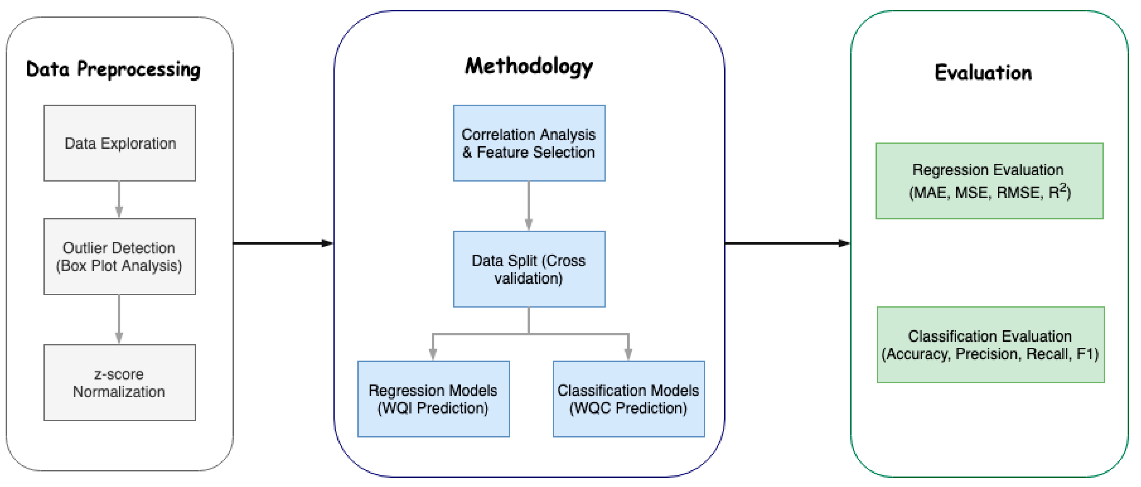
After all the data processing, for data analysis, several machine learning algorithms were employed to predict the WQI and WQC using the minimal number of parameters. Before applying a machine learning algorithm, there are some preliminary steps, like correlation analysis and data splitting, to prepare the data to be given as input to the actual machine learning algorithms.
3.7.1. Correlation Analysis
To find the dependent variables and to predict hard-to-estimate variables through easily attainable parameters, we performed correlation analysis to extract the possible relationships between the parameters. We used the most commonly used and effective correlation method, known as the Pearson correlation. We applied the Pearson correlation on the raw values of the parameters listed in
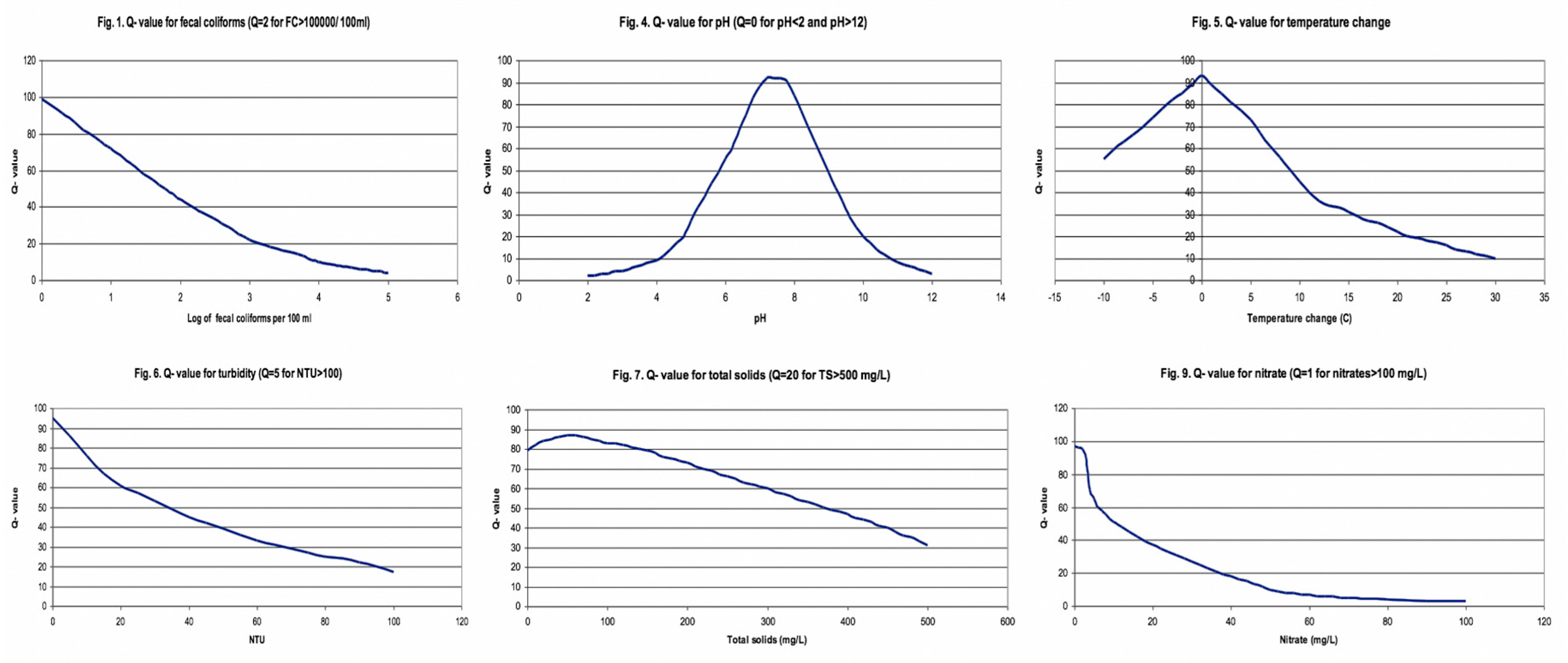
Table 4 and applied it after normalizing the values through q-value normalization as explained in the subsequent section.
As the correlation chart in
Table 4 indicates:
Alkalinity (Alk) is highly correlated with hardness (CaCO3) and calcium (Ca).
Hardness is highly correlated with alkalinity and calcium, and loosely correlated with pH.
Conductance is highly correlated with total dissolved solids, chlorides and fecal coliform count, and loosely correlated with calcium and temperature.
Calcium is highly correlated with alkalinity and hardness, while loosely correlated with TDS, chlorides, conductance and pH.
TDS is highly correlated with conductance, chlorides and fecal coliform, and loosely correlated with calcium and temperature.
Chlorides are highly correlated with conductance and TDS, and loosely correlated with temperature, calcium and fecal coliform.
Fecal coliform is correlated with conductance and TDS, and loosely correlated with chlorides.
Now that we have listed the correlation analysis observations, we find that our predicting parameter WQI is correlated with seven parameters, namely temperature, turbidity, pH, hardness as CaCO3, conductance, total dissolved solids and fecal coliform count. We have to choose the minimal number of parameters to predict the WQI, in order to lower the cost of the system. The three parameters whose sensors are easily available, cost the lowest and contribute distinctly to the WQI are temperature, turbidity and pH, which deems them naturally selected. The other convenient parameter is total dissolved solids, whose sensor is also easily available and is correlated with conductance and fecal coliform count, which means selecting TDS would allow us to discard the other two parameters. We leave the remaining inconvenient parameter, hardness as CaCO3, out because it is not highly correlated comparatively and is not easy to acquire.
To conclude the correlation analysis, we selected four parameters for the prediction of WQI, namely, temperature, turbidity, pH and total dissolved solids. We initially just considered the first three parameters, given their low cost, and if needed, TDS will be included later to analyze its contribution to the accuracy.
3.7.2. Data Splitting–Cross Validation
The last step prior to applying the machine learning model is splitting the provided data in order to train the model, test it with a certain part of the data and compute the accuracy measures to establish the model’s performance. This research explores the cross validation data splitting technique.
Cross validation splits the data into k subsets and iterates over all the subsets, considering k-1 subsets as the training dataset and 1 subset as the testing dataset. This ensures an efficient split and use of proper and definitive data for training and testing. This is generally computationally expensive, given the iterations, but our research uses a small dataset, which is mostly the case with water quality datasets, making cross validation more suited for this problem. We split the data into k = 6 subsets and ran cross validation. Therefore, as the complete training set consists of 663 samples, we ensured at least 100 samples for each fold subset, including the test set.
3.7.3. Machine Learning Algorithms
We used both regression and classification algorithms. We used the regression algorithms to estimate the WQI and the classification algorithms to classify samples into the previously defined WQC. We used eight regression algorithms and 10 classification algorithms. The following algorithms were employed in our study:
(1) Multiple Linear Regression
Multiple linear regression is a form of linear regression used when there is more than one predicting variable at play. When there are multiple input variables, we use multiple linear regression to assess the input of each variable that affects the output, as reflected in Equation (3), where
is the output for which machine learning has been applied to predict the value,
is the observed value,
is the slope on the observed value, and
is the error term [
17].
(2) Polynomial Regression
Polynomial regression is used when the relation between input and output variables is not linear and a little complex. We used a higher order of variables to capture the relation of input and output variables, which is not as linear. We used the order of two. Using a higher order of variables does carry the risk of overfitting, as reflected in Equation (4), where
is the output for which machine learning has been applied to predict the value,
is the observed value,
is the fitting value,
i is the number of parameters considered, k is the order of the polynomial equation, and
is the error term or residuals of the
ith predictor [
18]. We used it with 2-degree polynomials with an order of C.
(3) Random Forest
Random forest is a model that uses multiple base models on subsets of the given data and makes decisions based on all the models. In random forest, the base model is a decision tree, carrying all the pros of a decision tree with the additional efficiency of using multiple models [
19].
(4) Gradient Boosting Algorithm
This is the most contemporary algorithm used in most competitions. It uses an additive model that allows for optimization of differentiable loss function. We used it with a loss function of ‘ls’, a min_samples_split of 2 and a learning rate of 0.1 [
20].
(5) Support Vector Machines
Support vector machines (SVMs) are mostly used for classification but they can be used for regression as well. Visualizing data points plotted on a plane, SVMs define a hyperplane between the classes and extend the margin in order to maximize the distinction between two classes, which results in fewer close miscalculations [
21].
(6) Ridge Regression
Ridge regression works on the same principles as linear regression, it just adds a certain bias to negate the effect of large variances and to void the requirement of unbiased estimators. It penalizes the coefficients that are far from zero and minimizes the sum of squared residuals [
22,
23].
(7) Lasso Regression
Lasso regression works on the same principles as ridge regression, the only difference is how they penalize their coefficients that are off. Lasso penalizes the sum of absolute errors instead of the sum of squared coefficients [
24].
(8) Elastic Net Regression
Elastic net regression combines the best of both ridge and lasso regression. It combines the method of penalties of both methods and minimizes the loss function [
25].
(9) Neural Net/Multi-Layer Perceptrons (MLP)
Neural nets are loosely based on the structure of neurons. They contain multiple layers with interconnected nodes. They contain an input layer and output layer, and hidden layers in between these two mandatory layers. The input layer takes in the predicting parameters and the output layer shows the prediction based on the input. They iterate through each training data point and generalize the model by giving and updating the weight on each node of each layer. The trained model then uses those weights to decide what units to activate based on the input. Multi-layer perceptron (MLP) is a conventional model of neural net, which is mostly used for classification, but it can be used for regression as well [
26]. We used it for classification with the configuration of (3, 7) running for a maximum of 200 epochs using ‘lbfgs’ solver.
(10) Gaussian Naïve Bayes
Naïve Bayes is a simple and a fast algorithm that works on the principle of Bayes theorem with the assumption that the probability of the presence of one feature is unrelated to the probability of the presence of the other feature [
27].
(11) Logistic Regression
Logistic regression is a classification algorithm. It is based on the logistic function or the sigmoid function, hence the name. It is the most common algorithm used in the case of binary classification, but in our case we used multinomial logistic regression because there was more than two classes [
28]. We used it with ‘warn’ solver and l2 penalty.
(12) Stochastic gradient descent
This iterative optimization algorithm minimizes the loss function iteratively to find the global optimum. In stochastic gradient descent, the sample selection is random [
29].
(13) K Nearest Neighbor
The K nearest neighbor algorithm classifies by finding the given points nearest N neighbors and assigns the class of majority of n neighbors to it. In the case of a draw, one could employ different techniques to resolve it, e.g., increase n or add bias towards one class. K nearest neighbor is not recommended for large datasets because all the processing takes place while testing, and it iterates through the whole training data and computes nearest neighbors each time [
30]. We used a n = 5 configuration for our model.
(14) Decision Tree
A decision tree is a simple self-explanatory algorithm, which can be used for both classification and regression. The decision tree, after training, makes decisions based on values of all the relevant input parameters. It uses entropy to select the root variable, and, based on this, it looks towards the other parameters’ values. It has all the parameter decisions arranged in a top-to-down tree and projects the decision based on different values of different parameters [
31].
(15) Bagging Classifier
A bagging classifier fits multiple base classifiers on random subsets of data and then averages out their predictions to form the final prediction. It greatly helps out with the variance [
32].
We used default values for the algorithms, except MLP, which uses a (3, 7) configuration.


