A Monte-Carlo-Based Method for the Optimal Placement and Operation Scheduling of Sewer Mining Units in Urban Wastewater Networks

Abstract

Pressures on water resources, which have increased significantly nowadays mainly due to rapid urbanization, population growth and climate change impacts, necessitate the development of innovative wastewater treatment and reuse technologies. In this context, a mid-scale decentralized technology concerning wastewater reuse is that of sewer mining. It is based on extracting wastewater from a wastewater system, treating it on-site and producing recycled water applicable for non-potable uses. Despite the technology’s considerable benefits, several challenges hinder its implementation. Sewer mining disturbs biochemical processes inside sewers and affects hydrogen sulfide build-up, resulting in odor, corrosion and health-related problems. In this study, a tool for optimal sewer mining unit placement aiming to minimize hydrogen sulfide production is presented. The Monte-Carlo method coupled with the Environmental Protection Agency’s Storm Water Management Model (SWMM) is used to conduct multiple simulations of the network. The network’s response when sewage is extracted from it is also examined. Additionally, the study deals with optimal pumping scheduling. The overall methodology is applied in a sewer network in Greece providing useful results. It can therefore assist in selecting appropriate locations for sewer mining implementation, with the focus on eliminating hydrogen sulfide-associated problems while simultaneously ensuring that higher water needs are satisfied.

1. Introduction

Water scarcity problems have intensified considerably over the last decades. Rapid urbanization and population increase [1,2], water pollution and poor water management [3], as well as supply-side impacts of climatic changes [4,5], are the main causes of this problem. Moreover, technology advancement has improved living standards and consequently raised water demand. As existing technologies are often proven inadequate, a need for developing innovative water and wastewater collection, treatment and disposal practices emerges. In this direction, water reuse and reclamation approaches are constantly gaining ground. Reclaimed water is applicable for agricultural, urban and industrial uses and can also supplement existing water resources. Water reclamation helps alleviate the pressures on water resources and preserves environmental water quality. Furthermore, it reduces the costs associated with the development of new infrastructure and water transfer and treatment systems, as well as serves the need for a more sustainable use of water [6,7].

Interest is also focused on decentralized and satellite wastewater treatment technologies as an alternative to central treatment systems [8,9,10]. Central treatment systems have significant space and energy requirements which are often difficult to fulfill. Decentralized systems can be a smart solution to this problem. They are cost-effective and economical, since large capital costs are avoided. In addition, less pollutants, nutrients and contaminants emerge after decentralized wastewater treatment, thus human health and environmental risks are reduced [11]. An example of a mid-scale decentralized approach applicable at development level—up to 5000 households for instance—is that of sewer mining (SM) [12]. This technology is based on extracting wastewater out of a wastewater system and treating it on-site to produce recycled water. Some treatment by-products may be acceptable for return to the system under strict quality standards regarding sludge characteristics. These standards are determined in local consents or legislative provisions. The quality and quantity of the treatment by-products must have little or no detrimental effects on the wastewater system, taking into consideration the receiving sewer’s capacity, along with the wastewater quality characteristics downstream of the sludge return point [13]. The recycled water produced is appropriate for non-potable uses, such as irrigation of urban green areas, sports facilities and golf courses, toilet flushing and commercial and industrial applications (e.g., air conditioning, cooling towers etc.) [14,15,16]. The basic stages of sewer mining implementation can be seen in Figure 1.

Sewer mining schemes have been successfully set up in numerous cases worldwide [18,19,20], especially in Australia where the technology was pioneered [16,21,22,23,24]. Although the advantages of sewer mining are considerable, they are often overshadowed because of financial restrictions, inadequate frameworks and public skepticism about the use of recycled water in general [17,24]. Furthermore, the extraction of wastewater and the potential return of treatment by-products to the wastewater system affect the flow and the biochemical processes inside pipes downstream of the sewer mining application point [14]. One important challenge in particular is the alteration in hydrogen sulfide build-up inside sewers. Hydrogen sulfide (H₂S) is primarily responsible for odor, pipe corrosion and health-related problems.

In the present study, the Monte-Carlo method is combined with the United States Environmental Protection Agency’s Storm Water Management Model (SWMM) in order to address the problem of H₂S production in sewer networks. A tool for optimal SM unit placement in sewer networks is presented, aiming to minimize hydrogen sulfide production inside network pipes and, at the same time, to maximize the benefits from the technology application. After the identification of optimal locations for SM unit placement, the network’s response when sewer mining is applied and sewage is pumped out of the system is additionally examined. The study also deals with optimal pumping scheduling in terms of minimizing hydrogen sulfide production inside pipes downstream of the node out of which sewage is pumped. Two approaches are considered concerning optimal pumping scheduling. The study results are then used to draw useful conclusions regarding sewer mining application at a local scale.

2. Materials and Methods

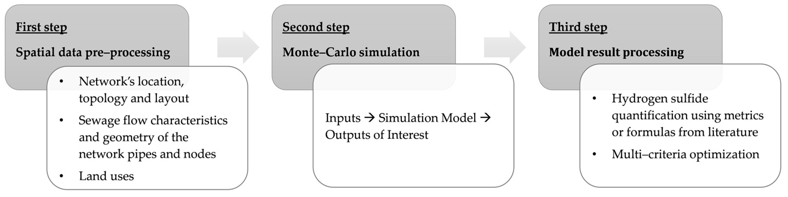
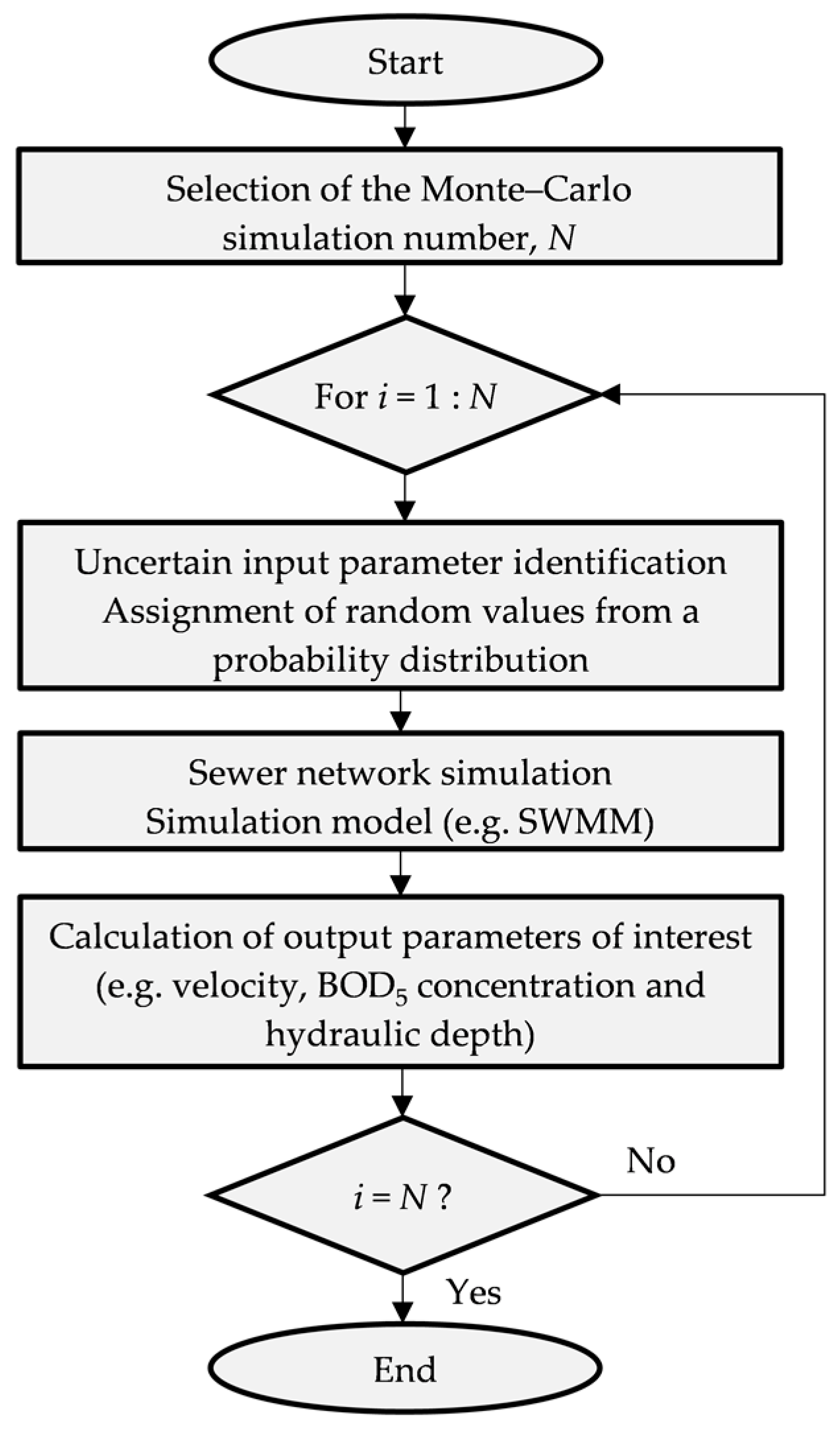
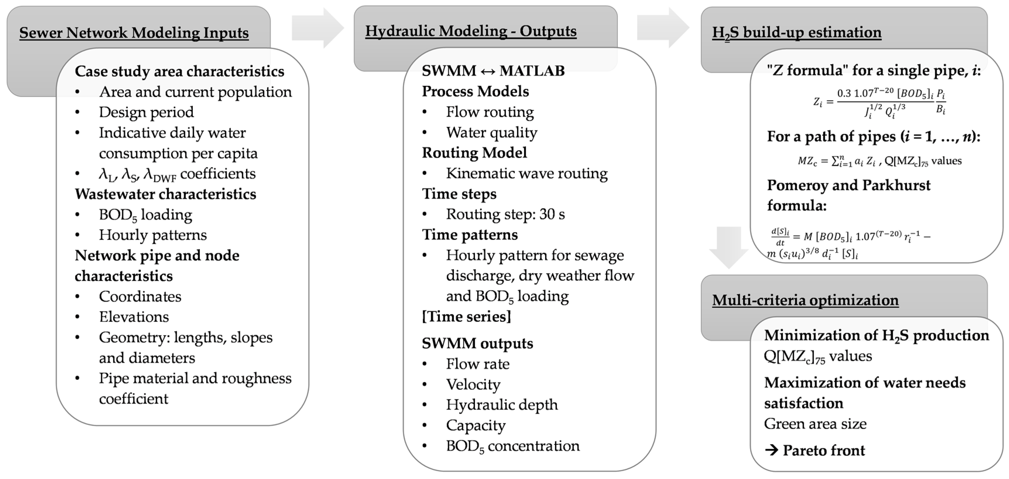
2.1. Methodology Description

The methodology for optimal SM unit placement in sewer networks is based on three main steps: spatial data pre-processing, Monte-Carlo simulation and model result processing, as shown in Figure 2.

The first step concerns collecting and pre-processing spatial data. Information about the network’s location, topology and characteristics is gathered at this stage. The network’s extent and layout, along with its connection to neighboring networks, treatment plants or water bodies are also determined. Knowledge about the sewage flow characteristics (e.g., flow rate, BOD₅ loading etc.) and the geometry (e.g., diameter, slope, length, elevation etc.) of the network pipes and nodes is required in this step. In addition, land uses in the vicinity of the network are identified. The focus is on areas that can possibly benefit from sewer mining implementation, such as green areas where recycled water is applicable for irrigation. Sewer mining equipment should be placed in close proximity so that the extracted sewage can be directly and efficiently transferred from the network to the treatment unit. To this end, network nodes that are more appropriate for SM unit placement are located. This procedure is based on setting a buffer zone of a certain width (10 m for instance) around each area, finding the network nodes situated within the limits of the zone and identifying the pipe path from each selected node to the network’s exit node. The aforementioned pipe path is unique for each network node due to the “collective nature” of sewer networks.

The second step includes developing a Monte-Carlo method and conducting multiple simulations using a simulation model such as the SWMM. The Monte-Carlo method is a stochastic procedure that propagates uncertainties related to input parameters such as daily and hourly flow coefficients and BOD₅ loading to the model outputs of interest. It also enables the expression of results in empirical models or probabilistic functions. The procedure begins by selecting a number of N simulations. For each simulation, uncertain input parameters are identified and assigned random values from a probability distribution. Afterwards, the simulation is carried out through the simulation model and parameters of interest, such as velocity, BOD₅ concentration and hydraulic depth, are calculated and stored for further processing. The Monte-Carlo simulation procedure is illustrated in Figure 3.

The third step regards model result processing. The aim is to address hydrogen sulfide build-up inside sewers, which is quantified using metrics (e.g., utility or risk functions) or formulas derived from literature. Afterwards, a multi-criteria optimization where two conflicting criteria are considered is executed. The first criterion concerns the minimization of hydrogen sulfide production inside network pipes. The second criterion concerns the maximization of the water needs satisfaction. A Pareto front is obtained through the optimization where optimal locations for sewer mining unit placement are determined. Other possible criteria for the optimization may refer to location suitability (e.g., minimization of the distance from the SM unit to the green area where the recycled water will be used), or may concern operation and transfer cost minimization as well as pump efficiency maximization. It should be mentioned that different decisions are required according to each case’s characteristics and restrictions. Multi-criteria analysis provides the option of using alternative metrics and criteria with respect to different aspects of the network. Therefore, it is a valuable tool in the modeling procedure.

After identifying potential locations for sewer mining unit placement, the way the network responds when the technology is implemented is examined. Regarding the modeling procedure, SM units placed in the sewer network are assumed to be additional network nodes. Moreover, an assumed network pipe can represent sewage extraction and transfer from the appointed network node to the SM unit. In the case where some treatment by-products return to the wastewater system, their transfer can be also taken into consideration by assuming a pipe that connects the SM unit to a network node downstream of the SM application point. The estimation of treatment by-product characteristics is possible if information concerning the influent characteristics (e.g., flow rate, velocity, BOD₅ concentration, temperature) and the treatment process and methods applied are available. At the design stage of a sewer mining scheme, formulas and models derived from literature can be used for this purpose. After the scheme set-up, important effluent characteristics must be measured and verified against laboratory results during a trial period. Data about pump capacity and hydraulic and geometric characteristics of the node and pipes mentioned above, should be provided as well. It is worth noting that adding new components to sewer networks changes their layout and structure, thus causing alterations in the modeling procedure (a different routing method may be required for example).

A simplified approach includes the creation of time-series regarding sewage flow and BOD₅ loading as an alternative option. On the one hand, time-series consisting of negative values represent sewage extraction and can serve as a form of output for the network. They are assigned to the network node out of which sewage is pumped. On the other hand, time-series with positive values represent the return of treatment residue to the network, thus serving as a form of input. These time-series are assigned to the network node where by-products end up.

In the present study, two different approaches are considered with respect to SM implementation in the case study network. The first approach assumes twenty-four-hour steady-rate pumping, while the second approach assumes twelve-hour steady-rate pumping between 8:00 a.m.–8:00 p.m. and no pumping for the remainder of the day. The same daily sewage amount pumped out of the network is considered for the two approaches. At first, sewage is pumped out of one network node only—one of the optimal nodes derived from the Pareto front. Afterwards, sewage is pumped out of two network nodes as two sewer mining units operate in two different areas simultaneously. It is assumed that treatment residue does not return to the network. A total of four different cases are examined and N simulations are conducted per case. In all cases, hydrogen sulfide production in the pipe routes from the nodes out of which sewage is pumped to the network’s exit node is quantified employing an empiric metric. Subsequently, the results are compared.

Optimal pumping scheduling can assist towards minimizing hydrogen sulfide production in sewer networks, since sewage extraction from the network alters the flow characteristics downstream of the technology application point. This study presents two approaches in the context of optimal pumping scheduling. The first approach assumes a ratio between the pumping flow rate and the sewage flow that ends up in the SM application node. A ratio coefficient, a, theoretically taking values from the interval (0, 1), is introduced to express this ratio. The ratio coefficient assumption is valid in cases where the sewage flow and the BOD₅ loading follow a similar hourly pattern. Scenarios where the ratio coefficient is set to 0.01 and 0.1 are subsequently examined and N simulations are run for each scenario. Furthermore, scenarios where the pumping rate is assumed steady—set to 50 m³/day, 100 m³/day and 200 m³/day—are considered for comparison purposes. Sewage is pumped out of one and afterwards out of two network nodes and it is assumed that treatment by-products do not return to the sewer network. Hydrogen sulfide production is then estimated regarding the pipe routes of the nodes out of which sewage is pumped to the network’s exit node. The network’s response is also studied when an appointed daily sewage amount is extracted according to the ratio coefficient assumption in comparison to steady-rate pumping application. The ratio coefficient is set to 0.5, a relatively high value, so as to easily detect the differences.

The second approach involves the employment of the genetic algorithm method regarding optimal pumping scheduling. Genetic algorithm optimizations are carried out for three different flow and BOD₅ loading scenarios that provide different hydrogen sulfide production results in the network pipes—minimum, moderate (estimated using the 50% quantile value of the empiric metric’s values obtained through the N simulations) and maximum production results. The day is divided into six four-hour periods and the pumping flow rates at the beginning and at the end of these periods are the problem’s variables. Linear interpolation is assumed at the intervals. The optimization criterion is the minimization of hydrogen sulfide production in the pipe route from the SM application point to the network’s exit node. Several restrictions are also determined, along with a set of values serving as initial population. The results are compared to those obtained through the simulations concerning the cases of no pumping and of the ratio coefficient assumption. The conclusions drawn from implementing genetic algorithm optimizations can serve as guidelines for further analysis with respect to optimal operation scheduling.

2.2. The Storm Water Management Model (SWMM)

The Storm Water Management Model (SWMM) is a dynamic rainfall–runoff model developed by the United States Environmental Protection Agency. It is applicable for single-event or long-term simulations of urban runoff quantity and quality. The SWMM model can be used for hydrologic and hydraulic simulations, as well as for flood control and water quality protection. It takes the precipitation in subcatchment areas into account and provides results concerning runoff and water quality by executing simulations where the time-step is user-defined. Runoff is transported through a system of pipes, channels, storage or treatment devices, pumps and regulators [25,26].

Regarding flow routing, the SWMM model provides three different routing options: Steady Flow, Kinematic Wave and Dynamic Wave Routing. In cases of partly filled conduits, all three routing methods employ Manning’s equation for flow rate calculation [25]:

$$Q=\frac{1}{n} A R^{2/3} S_{\mathrm{f}}^{1/2}$$

(1)

where Q (m³ s⁻¹) is the flow rate, n (s m^−1/3) is Manning’s roughness factor, A (m²) is the cross-sectional area of flow, R (m) is the hydraulic radius and S_f (m m⁻¹) is the friction slope.

The steady flow routing method is used when flow is deemed steady and uniform at every time-step of the simulation. Inflow hydrographs are transferred from the upstream to the downstream end of a conduit with no delay or change of shape. This routing method is the simplest among the three routing methods mentioned above and it is more appropriate for preliminary analysis [27].

The kinematic wave and dynamic wave routing methods concern unsteady flow and employ the Saint-Venant continuity (Equation (2)) and momentum (Equation (3)) equations.

$$\frac{\partial A}{\partial t}+\frac{\partial Q}{\partial x}=0$$

(2)

$$\frac{\partial Q}{\partial t}+\frac{\partial \left(Q^2/A\right)}{\partial x}+g A \frac{\partial H}{\partial x}+g A S_{\mathrm{f}}+g A h_{\mathrm{L}}=0$$

(3)

where Q (L³ T⁻¹) is the flow rate, A (L²) is the cross-sectional area of flow, x (L) is the distance along the conduit, t (T) is the time, H (L) is the hydraulic head of water in the conduit, S_f (L L⁻¹) is the friction slope, h_L (L) is the local energy loss per unit length and g (L T⁻²) is the acceleration of gravity.

More specifically, the kinematic wave routing method is used in the cases where flow is considered unsteady and uniform. According to Miller [28], this method can be applied when the wave is deemed long and flat so as to assume that the friction slope, S_f, is nearly equal to the bed slope, S₀. In this method, the complete Saint-Venant continuity equation and a simplified form of the Saint-Venant momentum equation, where the water surface slope is assumed equal to the conduit slope (S₀ ≈ S_f), are solved for each conduit. Outflow hydrographs are delayed and attenuated. The kinematic wave method is strictly applicable in dendritic networks and can provide sufficient results in long-term simulations [25].

The dynamic wave routing method is applied when flow is considered unsteady and varied. It employs the complete Saint-Venant continuity and momentum equations, along with an additional equation regarding the nodes of the network [29]. This equation calculates the change in hydraulic head at a certain node with respect to time as follows:

$$\frac{\partial H}{\partial t}=\frac{{{\displaystyle \sum }}^{\text{}}Q}{A_{\mathrm{store}}+{{\displaystyle \sum }}^{\text{}}{A}_{\mathrm{s}}}$$

(4)

where A_store is the surface area of the node itself, ΣA_s is the surface area contributed by the conduits connected to the node and ΣQ is the net flow into the node-namely, inflow minus outflow-contributed by all conduits connected to the node along with any externally imposed inflows.

The dynamic wave routing method is the most complex among the three routing methods and can account for channel storage, backwater effects, entrance or exit losses and pressurized flow, so it is applicable for any network layout. This method provides accurate results yet requires small time-steps—usually smaller than 30 s—and it is generally time-consuming [25].

Selecting the most appropriate routing method depends on many factors in accordance with each case’s restrictions, including the network’s age. In new or relatively new sewer networks where sewage flow can be assumed uniform and unsteady, the kinematic wave routing method is deemed adequate. On the contrary, in old sewer networks, flow is considered unsteady and varied because of sediment accumulation and pipe corrosion. Consequently, dynamic wave routing is required [27].

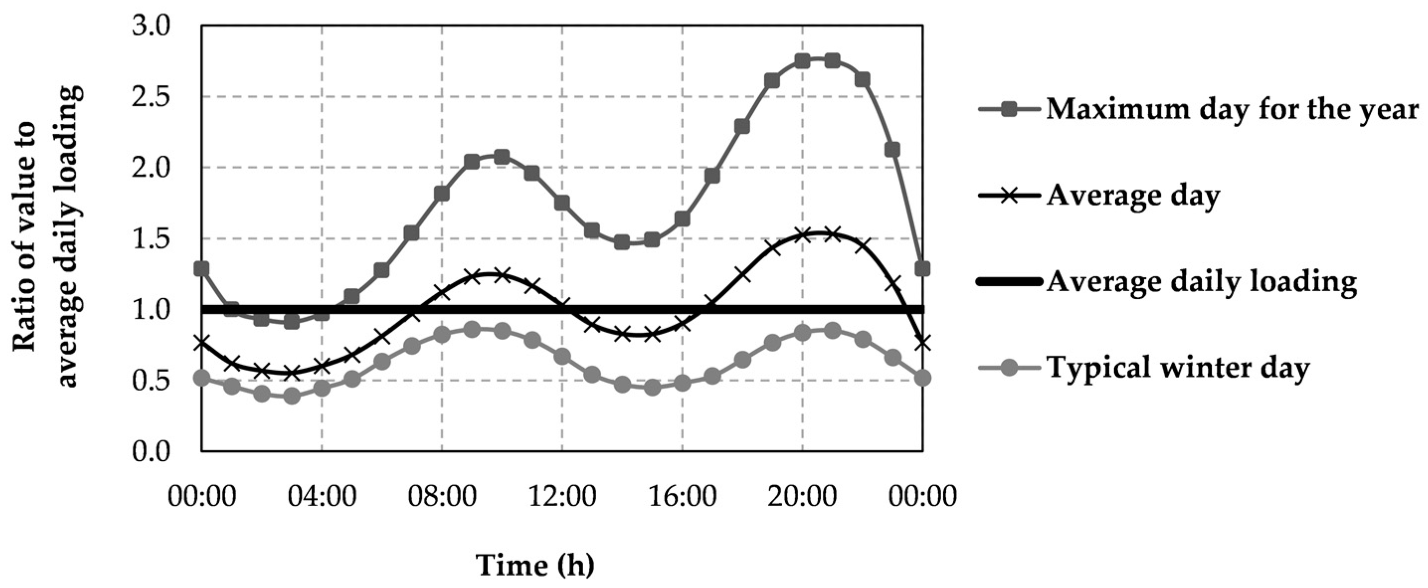
2.3. Design Discharge Calculation

Total design discharge (Q_D), which is used to assess the network performance, is calculated as the sum of sewage discharge (Q_s) and dry weather flow (Q_DWF). Sewage discharge is given by Equation (5) [30,31,32]:

$$Q_{\mathrm{s}}=\frac{q E}{86400} {\lambda }_{\mathrm{L}} {\lambda }_{\mathrm{S}} {\lambda }_1 {\lambda }_2$$

(5)

where Q_s (L s⁻¹) is the sewage discharge, q (L day⁻¹ cap⁻¹) is the indicative daily water consumption per capita, E (cap) is the serviced population, λ_L (–) is a loss coefficient of the water distribution network, λ_S (–) is a coefficient about the water percentage that ends up in the sewage network through runoff, λ₁ (–) is a seasonal coefficient and λ₂ (–) is a coefficient of peak discharge.

Dry weather flow can be calculated with respect to sewage discharge as follows [30]:

$$Q_{\mathrm{DWF}}=Q_{\mathrm{s}} {\lambda }_{\mathrm{DWF}}$$

(6)

where Q_DWF (L s⁻¹) is the dry weather flow and λ_DWF is a dry weather coefficient (set to 0.2 in this study).

In Equation (5), the values of coefficients λ_S, λ_L, λ₁ and λ₂ vary from case to case due to differences that depend on many factors, such as the network’s type, age and location, as well as the population and its living standards, which affect water demand and use. Local conditions should be taken into account when selecting appropriate values for these coefficients. It is preferable to use historical data concerning the study area, provided that it is reliable and that it covers a sufficient amount of time. However, when data is not available, the coefficients are assigned values determined from literature. Additionally, both sewage discharge and dry weather flow values regarding each network node are multiplied by the values of an hourly pattern so that hourly flow fluctuations are taken into account.

2.4. Hydrogen Sulfide Build-Up Estimation

Sulfide can be found in solution inside sewers as a mixture of H₂S and HS⁻, when wastewater pH takes normal values between 6.5 and 8. Sulfide ion, S²⁻, is also present in the wastewater, yet its concentration is insignificant for pH values under 12. In cases of specific pH, temperature and flow conditions inside a pipe, an amount of hydrogen sulfide is emitted in the pipe’s atmosphere. In the presence of oxygen and moisture on exposed pipe walls, H₂S is oxidized and sulfuric acid is produced [33]. As a result, hydrogen sulfide is related to pipe corrosion. Apart from this, it is responsible for odor problems, as well as human health-related effects including headaches, nausea, respiratory injury and—in extreme cases—immediate death [34].

Although there are several studies regarding H₂S build-up prediction, such as those by Pomeroy, Thistlethwayte and Boon and Lister [35,36,37], only a few deal with its emission in the sewers’ atmosphere. According to Lahav et al., the existing studies are divided into two main categories. The first category includes empirical models where H₂S emission is linked to flow and turbulence conditions [38]. The Pomeroy–Parkhurst equation which is used to estimate total sulfide concentration inside sewers is an example [39]. The second category concerns the employment of sewer re-aeration models where the gas transfer coefficient of sulfide replaces the gas transfer coefficient of oxygen [38]. The study of Yongsiri et al. [40] belongs to this category. In the study of Lahav et al., concepts from the mixing theory are adapted and an emission equation is presented [38].

Taking into account the available data and adopting a simpler approach at the first stage of the model application, the ‘Z formula’, an empirical formula developed by Pomeroy, is used in this study to predict hydrogen sulfide build-up inside each network pipe [33,41]:

$$Z_i=\frac{0.3 {1.07}^{T-20} {\left[BO{D}_5\right]}_i}{J_i^{1/2} Q_i^{1/3}}\frac{P_i}{B_i}$$

(7)

where Z is a dimensionless metric that quantifies hydrogen sulfide build-up probability, i is the pipe index, T (°C) is the sewage temperature, BOD₅ (mg L⁻¹) is the five-day concentration of Biochemical Oxygen Demand, J (m m⁻¹) is the pipe slope, Q (m³ s⁻¹) is the discharge, P (m) is the wetted perimeter of the pipe wall and B (m) is the surface width of the stream.

As stated by Bielecki and Schremmer, a threshold concerning the Z metric values is set to 7500 (Z_limit = 7500). That is to say, the Z metric value in a pipe must be lower than or equal to 7500 so that critical conditions concerning H₂S production are avoided [41].

According to Tsoukalas et al., in the case of a “chain” of pipes instead of a single pipe, a modified index can be used [30,31,32]:

$$M{Z}_{\mathrm{c}}={\displaystyle \sum }_{i=1}^n{a}_i Z_i$$

(8)

where a_i is a weight coefficient concerning pipe i. In the present study, this coefficient is calculated with respect to each pipe using the formula a_i = L_i/L_tot, where L_i is the length of pipe i, and L_tot is the total length of the chain’s pipes i = 1, …, n.

Equation (7) provides a general picture about hydrogen sulfide production inside sewers in order to identify network pipes where potential problems can arise. However, further analysis is necessary to ensure more accuracy. To this end, the Pomeroy and Parkhurst empiric equation mentioned before is employed to estimate total sulfide concentration inside each network pipe [39,42]. It is suggested that total sulfide concentration must not exceed the threshold of 1 mg/L so as to avoid critical conditions [41,43]. The Pomeroy and Parkhurst equation is as follows:

$$\frac{d{\left[S\right]}_i}{dt}=M {\left[BO{D}_5\right]}_i {1.07}^{\left(T-20\right) }{r}_i^{-1}-m {\left(s_i{u}_i\right)}^{3/8} d_i^{-1} {\left[S\right]}_i$$

(9)

where i is the pipe index, S (mg L⁻¹) is the total sulfide concentration in the aqueous phase, t (h) is the retention time, r (m) is the hydraulic radius, s (m m⁻¹) is the pipe slope, u (m s⁻¹) is the velocity of the stream and d (m) is the mean hydraulic depth. In cases of partially filled pipes, empirical constants M and m are equal to 0.32 × 10⁻³ m h⁻¹ and 0.64 (s m⁻¹)^3/8 h⁻¹ respectively (conservative form). Parameters BOD₅ and T have been already defined in Equation (7).

2.5. Case Study

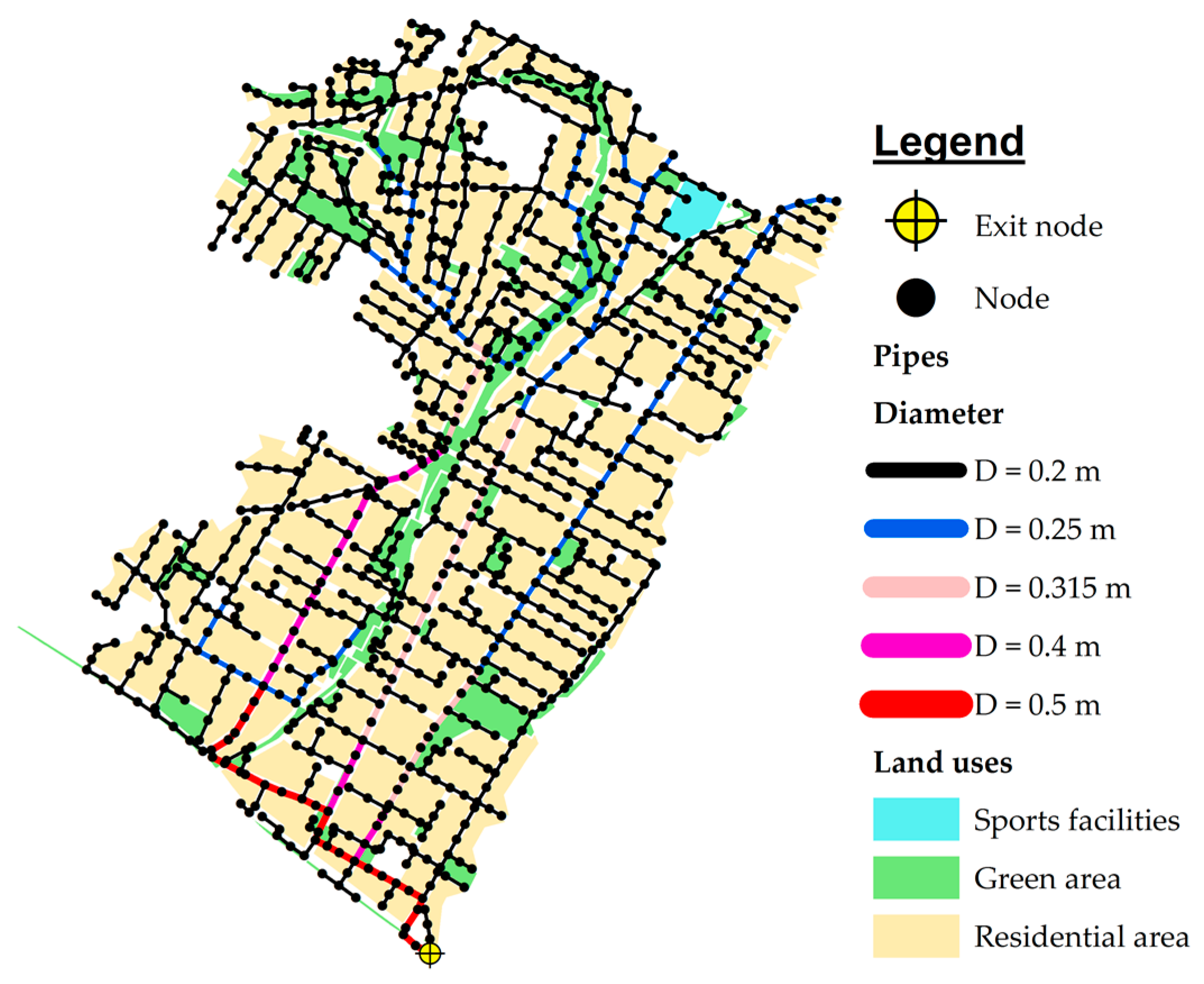
2.5.1. Study Area

The case study is based on a sewer network designed for future construction in the town of Kalyvia Thorikou in East Attica, Greece. It is part of a larger engineering project of the Saronikos municipality concerning the extension of the coastal zone’s existing sewer network. The sewer network is foreseen to accommodate a total area of about 118 hectares, consisting of 98 hectares of residential areas, 19 hectares of green areas and one hectare of sports facilities. The serviced population is 10–15 thousand people. The case study network has a total length of approximately 38 km and includes 1030 pipes and 1031 nodes, one of which is the network’s exit node. The network pipes have diameters ranging between 0.2–0.5 m and slopes ranging between 2 and 150‰. The case study sewer network is shown in Figure 4.

2.5.2. Implementation Details

The design period of the network is set to T = 40 years and the design population is calculated by Equation (10):

$$P_t=P_0{\left(1+r\right)}^t$$

(10)

where P₀ is the current population, r is the increase rate (assumed 1.5% in this study) and t is the extrapolation year (t = 0, …, T).

The population that corresponds to each network node is calculated for the design period according to Equation (10). It is afterwards used for the total discharge calculation concerning each network node (Equations (5) and (6)). The values of coefficients λ_L and λ_S in Equation (5) are set respectively to 0.85 and 0.65 for t = 40 years—the design period. Coefficients λ₁ and λ₂ are deemed uncertain and independent—that is to say, their covariance is zero. In the context of the Monte-Carlo method, they are assigned random values from the uniform distribution in the interval [0.5, 2]. As for the BOD₅ loading, six different cases are considered in the model simulations: 40, 45, 50, 55, 60 and 65 g/cap/day. In order to calculate the BOD₅ loading (in g/day) that corresponds to each network node, these values are multiplied by the node’s population. The total design discharge, the dry weather flow and the BOD₅ loading of the network nodes are inputs for the simulation model. In the study of Metcalf & Eddy Inc. (Wakefield, MA, USA) et al. [44], information about wastewater flow and BOD₅ hourly fluctuations is presented. According to this information, an hourly pattern regarding flow and BOD₅ fluctuations adapted to local conditions is assumed. The same hourly pattern is considered for sewage discharge, dry weather flow and BOD₅ loading and is shown in Figure 5. It is worth noting that the average day hourly pattern is used in the SWMM calculations.

A total of N = 120 simulations for N different loading scenarios are conducted using the SWMM model. The analysis is carried out on a twenty-four-hour basis and concerns both flow routing and water quality modeling. At this stage, it is assumed that no significant losses occur to the wastewater system (in comparison to the amounts of sewage transported through the network pipes). Sediment accumulation and pipe corrosion are also considered minimal. Therefore, the kinematic wave routing method is deemed appropriate for the analysis and the simulation time-step is set to 30 s. The simulations are executed through the MATLAB environment where results of interest inside each network pipe are stored for further processing.

Equation (7) is applied to each time-step of the N simulations run and to each network pipe, assuming the temperature value equal to 18 °C. The Monte-Carlo method allows results to be expressed in reliability functions. Accordingly, a reliability level of x = 75% is chosen and the corresponding quantile, Q[Z_i]_{x = 75}, is calculated for each pipe, i. This quantity expresses that the x = 75% of the Z_i values resulting from the N simulations with respect to pipe i is lower than or equal to the quantile value.

Equation (9) is also applied for each network pipe, assuming an initial total sulfide concentration of 0.2 mg/L. Regarding parameters of Equation (9) that vary from scenario to scenario, the corresponding quantile values for the same reliability level (x = 75%) are employed.

In addition, Equation (8) is employed in order to calculate the MZ_c values in each pipe route of interest. More specifically, the MZ_c values are calculated for pipe routes from nodes that have already been selected as more appropriate for SM unit placement to the network’s exit node. The quantile Q[MZ_c]_{x = 75} is also calculated for these pipe routes. The recycled water produced from the SM technology application is designated for green area irrigation. Thirty-eight green areas can be found in the vicinity of the network (Figure 4). In each green area, the node with the lowest Q[MZ_c]₇₅ value among all nodes of the area is identified. Pipe routes from identified nodes to the network’s exit node present lower hydrogen sulfide build-up probabilities compared to discarded nodes. The search for potential locations concerning SM unit placement is therefore focused on these nodes.

A multi-criteria optimization where two criteria are determined is subsequently carried out. The first criterion is the minimization of hydrogen sulfide production, expressed through lower Q[MZ_c]₇₅ values, and the second criterion is the maximization of the water needs satisfaction. In the absence of actual data, area size is used as an approximate indicator of the irrigation water demand regarding each green area. Consequently, the optimization’s second criterion translates into maximizing the size of the green area that can possibly benefit from SM implementation. A Pareto front in which the locations for optimal SM unit placement are identified is then created. Figure 6 summarizes the modeling procedure and components.

Subsequently, the cases where sewage is extracted from the identified optimal network nodes are examined. In these cases, the modeling procedure described above is the same except the addition of several time-series in the SWMM model. Initially, sewage is pumped out of one network node only. Afterwards, two SM units are placed in two different areas while operating simultaneously and sewage is pumped out of two network nodes. Time-series with negative values concerning sewage flow and BOD₅ loading are inputs to the model and represent sewage extraction. These time-series are assigned to the corresponding network nodes from which sewage is extracted and their values are adapted according to the pumping schedule applied.

It is also worth noting that when employing the genetic algorithm method for optimal pumping scheduling, the procedure can be quite time-consuming. For this reason, the simulation time-step is changed from 30s to 120 s, so as to alleviate the computational burden.

3. Results

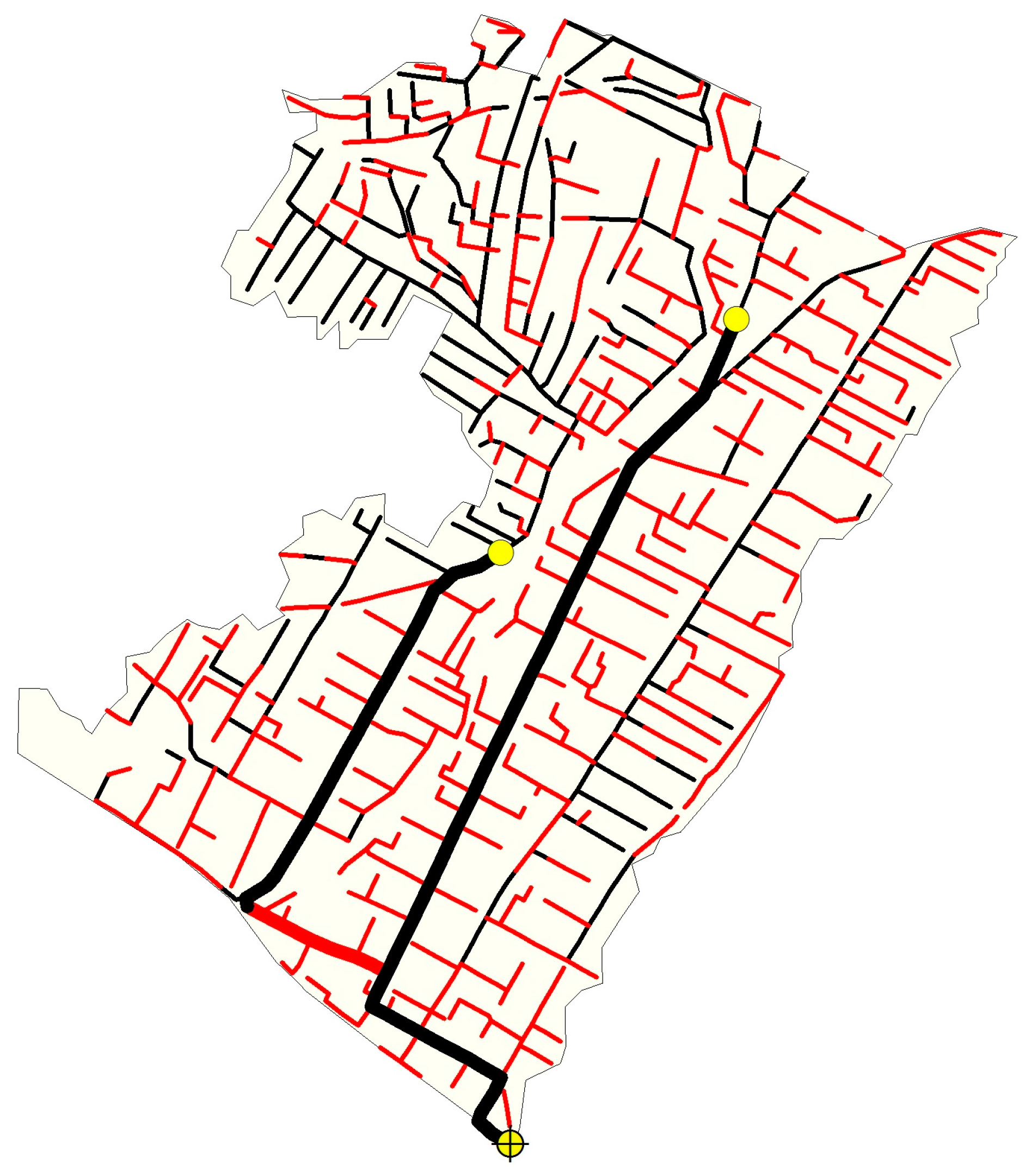
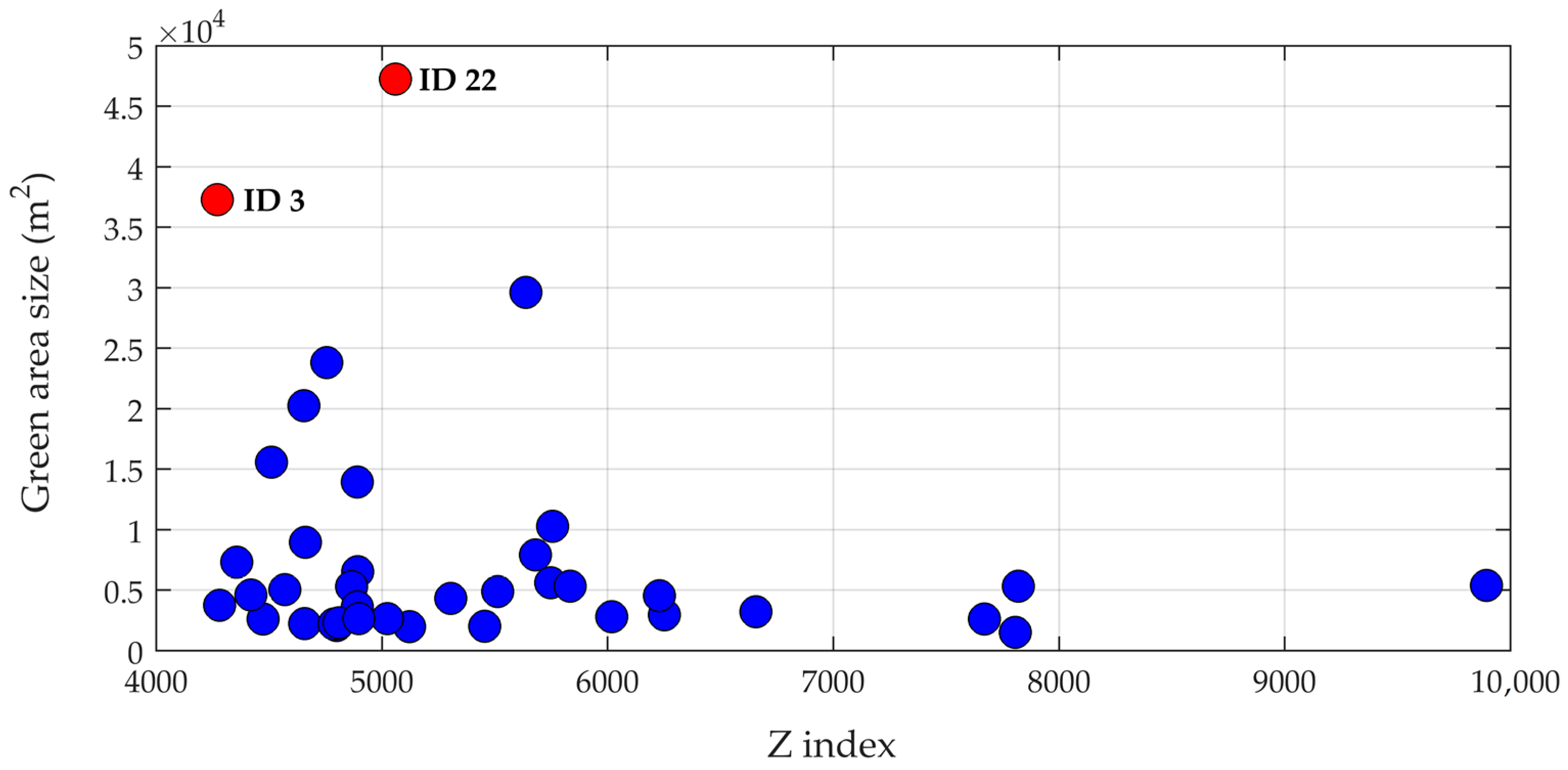
3.1. Identification of Locations for Optimal Sewer Mining Unit Placement

The N simulations executed provide results that are used for the multi-criteria optimization. Optimal areas for SM unit placement are then depicted in a Pareto front obtained through the optimization (Figure 7). X Axis shows the Z index values, namely the Q[MZ_c]₇₅ values that correspond to each green area. Y Axis shows green area size in square meters. The dots correspond to green areas where the network nodes that are potential locations for SM unit placement can be found. More specifically, red dots are non-dominated solutions of the Pareto front. That is to say, they correspond to green areas including nodes that are optimal locations for sewer mining application. These are areas ID 3 and ID 22. Blue dots correspond to the discarded green areas.

Figure 8 shows areas ID 3 and ID 22 marked in red. These areas include the optimal nodes for SM unit placement, marked in yellow. The optimal pipe paths—namely, the pipe paths which have the minimum Q[MZ_c]₇₅ values—from the optimal nodes of areas ID 3 and ID 22 to the network’s exit node are marked in black.

Figure 9 presents the network’s pipes marked in different colors according to whether the Q[Z_i]₇₅ values that resulted from the N simulations exceed the Z ≤ 7500 threshold or not. If the threshold is exceeded, the pipe is marked in red. Otherwise, it is marked in black.

It is observed that the Z ≤ 7500 threshold is exceeded in numerous network pipes. As mentioned in Section 2.4, the Z metric is empirical and aims at identifying pipes where critical conditions concerning hydrogen sulfide production may occur, thus requiring specific measures. Furthermore, most pipes where the threshold is exceeded have smaller slopes or receive smaller inflows from their corresponding upstream nodes compared to the other network pipes. This results in higher Z metric values according to Equation (7).

Figure 10 regards hydrogen sulfide build-up in the pipe path from the optimal node of area ID 3 to the network’s exit node. Figure 10a depicts the Q[Z_i]₇₅ values that resulted from the N simulations in all pipes of the path. It indicates pipes where problems related to H₂S production may appear—namely, pipes where the corresponding Q[Z_i]₇₅ values approach or exceed the Z ≤ 7500 threshold—and frequent checks may be needed so as to avoid critical conditions in the future. It is observed that Q[Z_i]₇₅ values are greater than 6000 in pipes C171–C168, yet the threshold is not exceeded in any pipes of the optimal pipe path. Figure 10b depicts the non-exceedance probability of the Z ≤ 7500 threshold. The calculations are based on the empirical distribution function for the sample of Z metric values obtained through the N simulations concerning each network pipe. High reliability levels are achieved, as non-exceedance probability values are higher than 90%. Finally, Figure 10c illustrates total sulfide concentration inside the path’s pipes, calculated according to Equation (9). Total sulfide concentration in all pipes does not exceed the limit of 1 mg/L, so no critical conditions are expected.

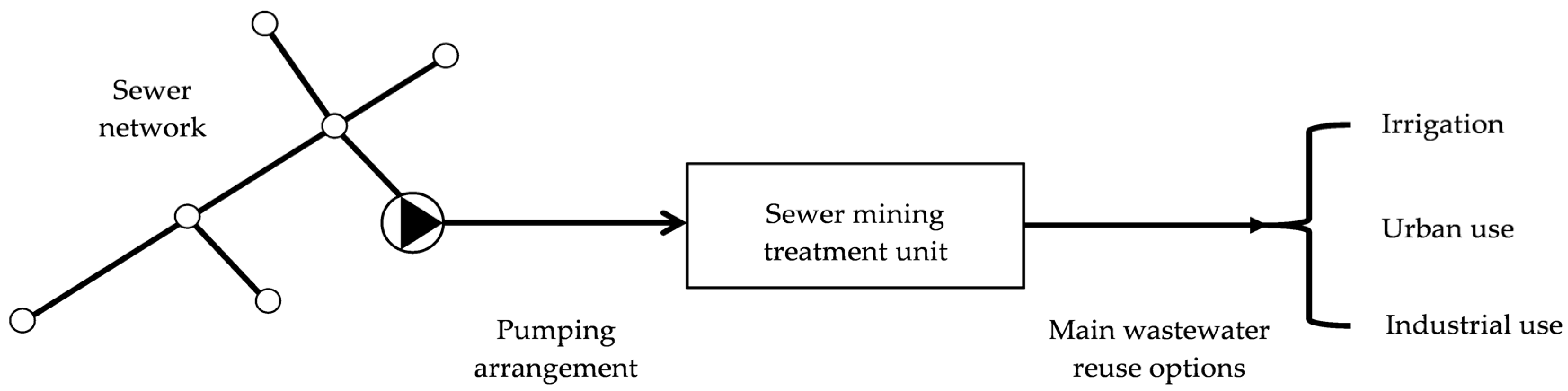
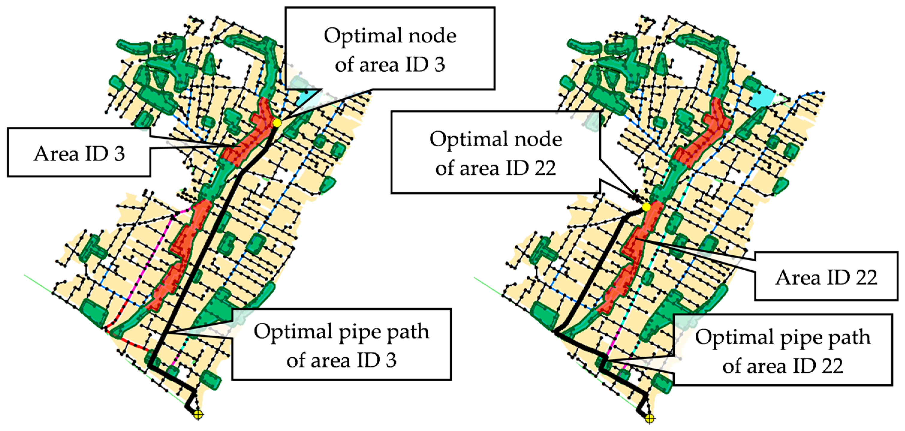
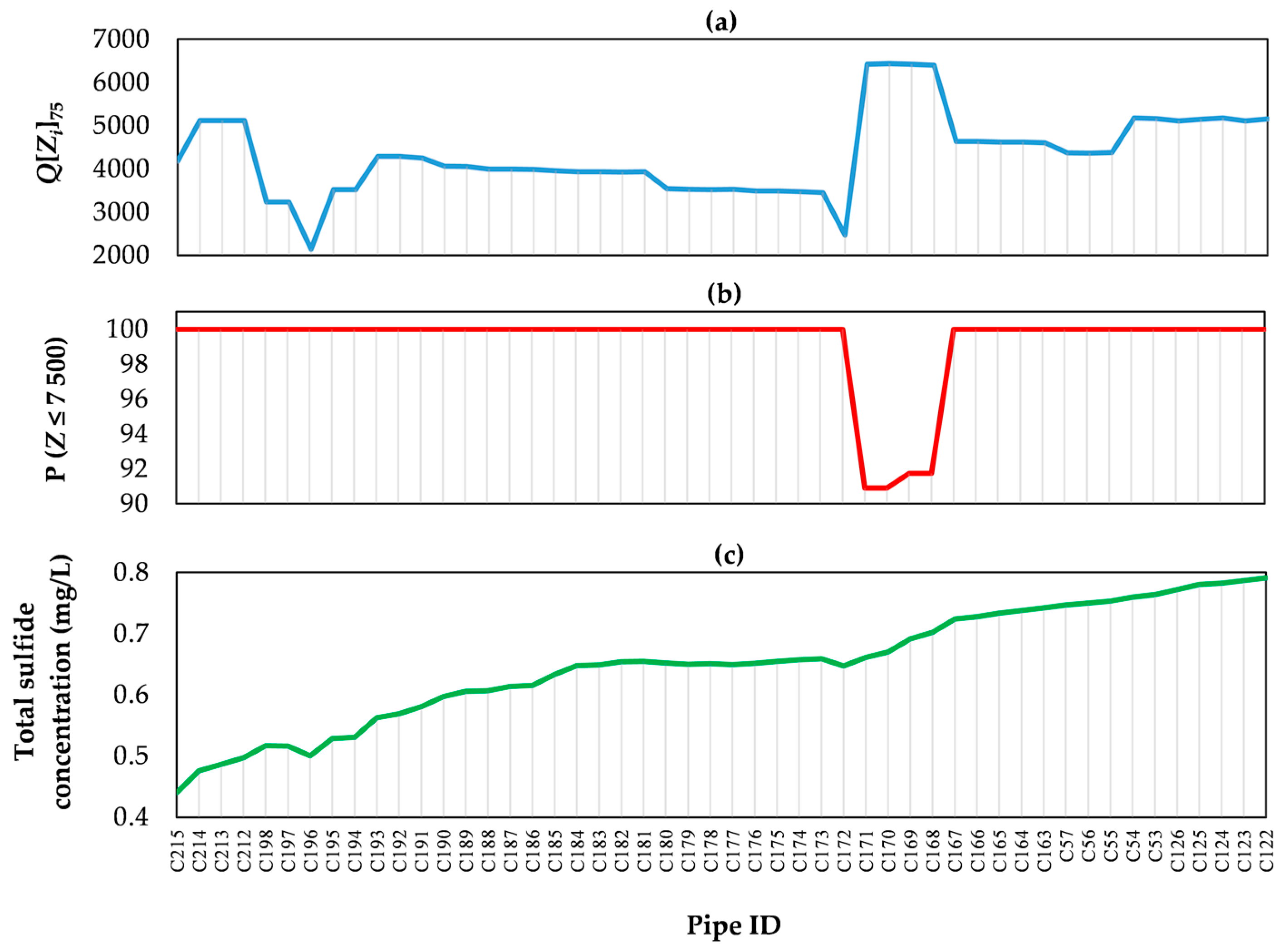
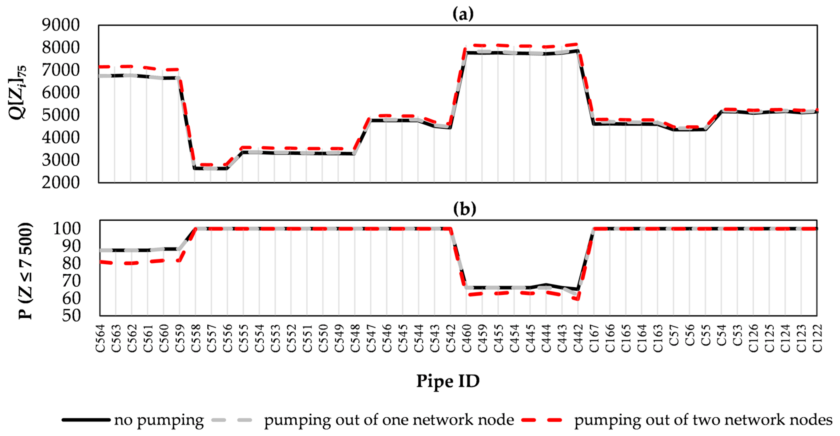
3.2. Sewer Mining Implementation in the Sewer Network

After the identification of the locations for optimal SM unit placement as discussed in Section 2.1, the way the network responds when sewage is extracted from it is also examined. As stated before, two different pumping schedules are applied: continuous steady-rate pumping for a twenty-four-hour period and continuous steady-rate pumping between 8:00 a.m.–8:00 p.m., assuming no pumping for the remainder of the day. The daily sewage amount extracted from the system is set to 100 m³ in both cases. At first, it is assumed that sewer mining is applied in area ID 3 only, so sewage is pumped out of the optimal node of this area. Subsequently, it is considered that sewer mining is applied in both areas ID 3 and ID 22 and that sewage is pumped out of their corresponding optimal nodes at the same time.

Figure 11 and Figure 12 show the Q[Z_i]₇₅ values and the non-exceedance probability of the Z ≤ 7500 threshold across pipe routes from the optimal nodes of areas ID 3 and ID 22 to the network’s exit node respectively. The results presented in these figures regard steady-rate pumping for a twenty-four-hour period in the case of two different pumping approaches and are compared to the corresponding results when no pumping takes place—in other words, when sewer mining is not applied in the network.

In Figure 11a, higher Q[Z_i]₇₅ values are observed when sewage is pumped out of the network in comparison to when no pumping takes place. The differences are more noticeable in the cases where Q[Z_i]₇₅ values are already high and close to the threshold value when no pumping occurs (pipes C171–C168 for instance). While conducting the N simulations, parameters J and T remain unchanged in Equation (7), whereas parameters BOD₅, P, B and Q vary per simulation regarding a specific pipe. However, changes in BOD₅ concentration are insignificant, as it is assumed that treatment residue does not return to the network. Consequently, changes in the Z metric are mainly affected by sewage flow alterations. When pumping occurs, the flow decreases due to sewage extraction and the Z metric values decrease accordingly. In downstream pipes close to the network’s exit node, differences between Q[Z_i]₇₅ values in the three cases examined are slight. Because of the sewer network’s collective nature, these pipes conduct considerably larger sewage flows compared to the other network pipes. In addition, no pumping occurs out of any other nodes closer to the network’s exit node. Differences can be also observed between Q[Z_i]₇₅ values when sewage is pumped out of one node only in comparison to when sewage is extracted from two nodes at the same time. In the latter case, an increase of the metric’s values is observed in the common section of the pipe paths from these two nodes to the network’s exit node (pipes C167–C122). Indeed, pumping sewage out of one optimal node does not affect the upstream pipes of the other node’s pipe path.

In Figure 12a, the Q[Z_i]₇₅ values derived from the non-pumping scenario and those from the scenario where sewage is pumped out of one node only are identical in the upstream nodes of the optimal pipe route of area ID 22 (pipes C564–C442) and begin to differ in the common section of the optimal pipe routes of both areas ID 3 and ID 22 (pipes C167–C122). Moreover, Q[Z_i]₇₅ values increase when sewage is also pumped out of the optimal node of area ID 22, as is expected.

Figure 11b and Figure 12b show the non-exceedance probability of the Z ≤ 7500 threshold across the optimal path. Generally, when sewage is pumped out of the network, a decrease in the non-exceedance probability values is expected. This decrease is more significant in the cases where reliability levels are already reduced in the non-pumping case (pipes C171–C168 in Figure 11b and pipes C460–C442 in Figure 12b for example). Furthermore, the non-exceedance probability decreases further in the pipes closer to the sewage extraction point. If the daily sewage amount pumped out of the network increases, it is expected that the observed decrease in these pipes will become more acute and that a wider range of pipes will be affected.

Similar conclusions can be drawn with respect to pumping between 8:00 a.m.–8:00 p.m. Figure 13’s aim is to compare the non-exceedance probability values regarding the N loading scenarios examined for three pipes of interest in the cases of twenty-four-hour and twelve-hour pumping. More specifically, the two pipes downstream of the optimal nodes of areas ID 3 and ID 22 are examined, along with the network’s exit pipe. Figure 13 concerns pumping out of both the optimal nodes of areas ID 3 and ID 22. It can be noted that in the case of pumping between 8:00 a.m.–8:00 p.m., the non-exceedance probability values in the three pipes are lower compared to the corresponding values in the case of twenty-four-hour pumping. The differences regarding the network’s exit pipe are slight due to the reasons mentioned before. Nevertheless, values in the pipe downstream of the optimal node of area ID 3 are noticeably decreased in the case of twelve-hour pumping. Indeed, the Z ≤ 7500 threshold is exceeded in some scenarios. When steady-rate pumping occurs for a twelve-hour period instead of a twenty-four-hour period and the same daily sewage amount is extracted from the network, pumping flow rate is doubled. In addition, the flow inside the pipe downstream of the optimal node of area ID 3 is smaller than the one inside the other two pipes examined. Consequently, changes in non-exceedance probability values concerning this pipe are more significant.

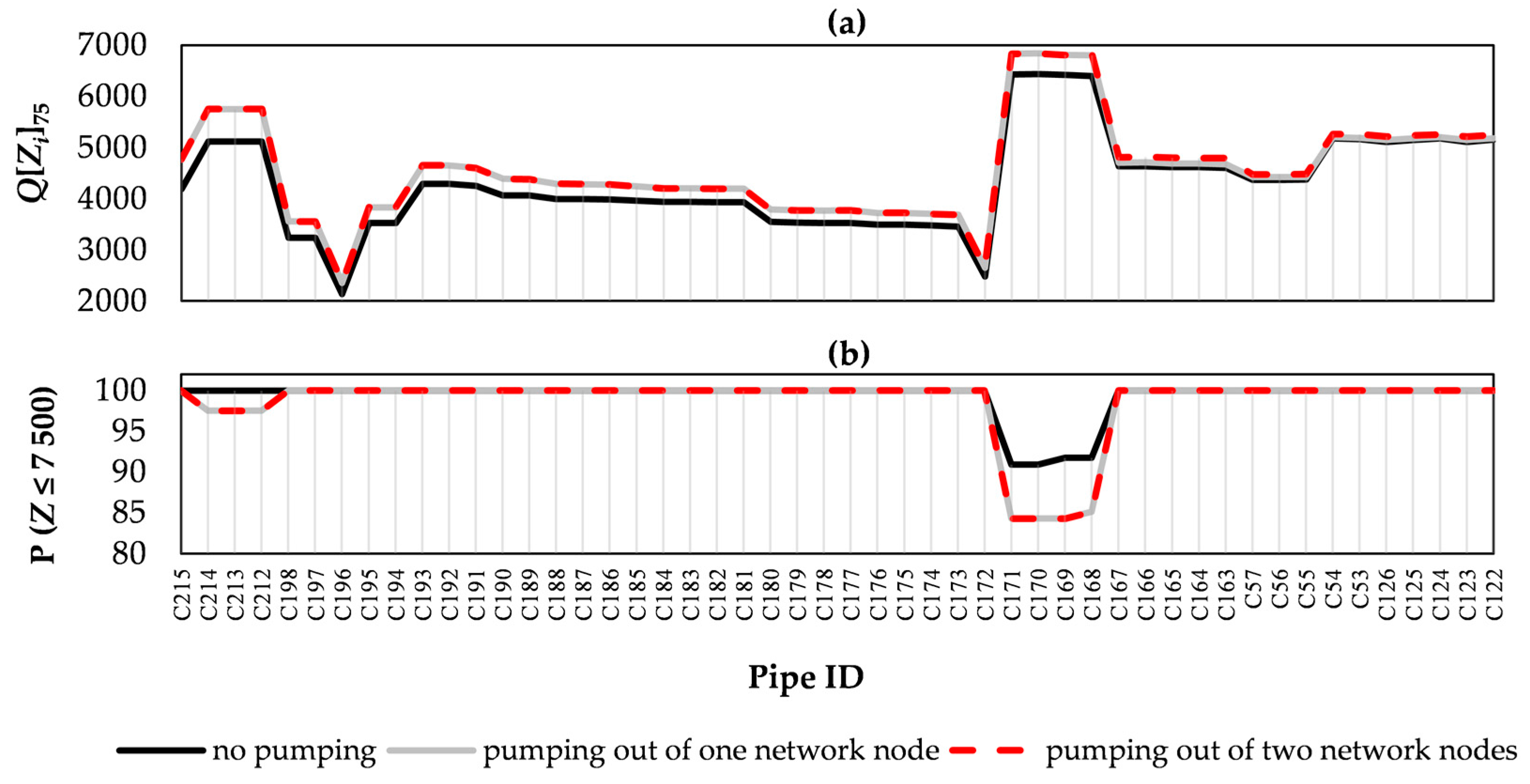
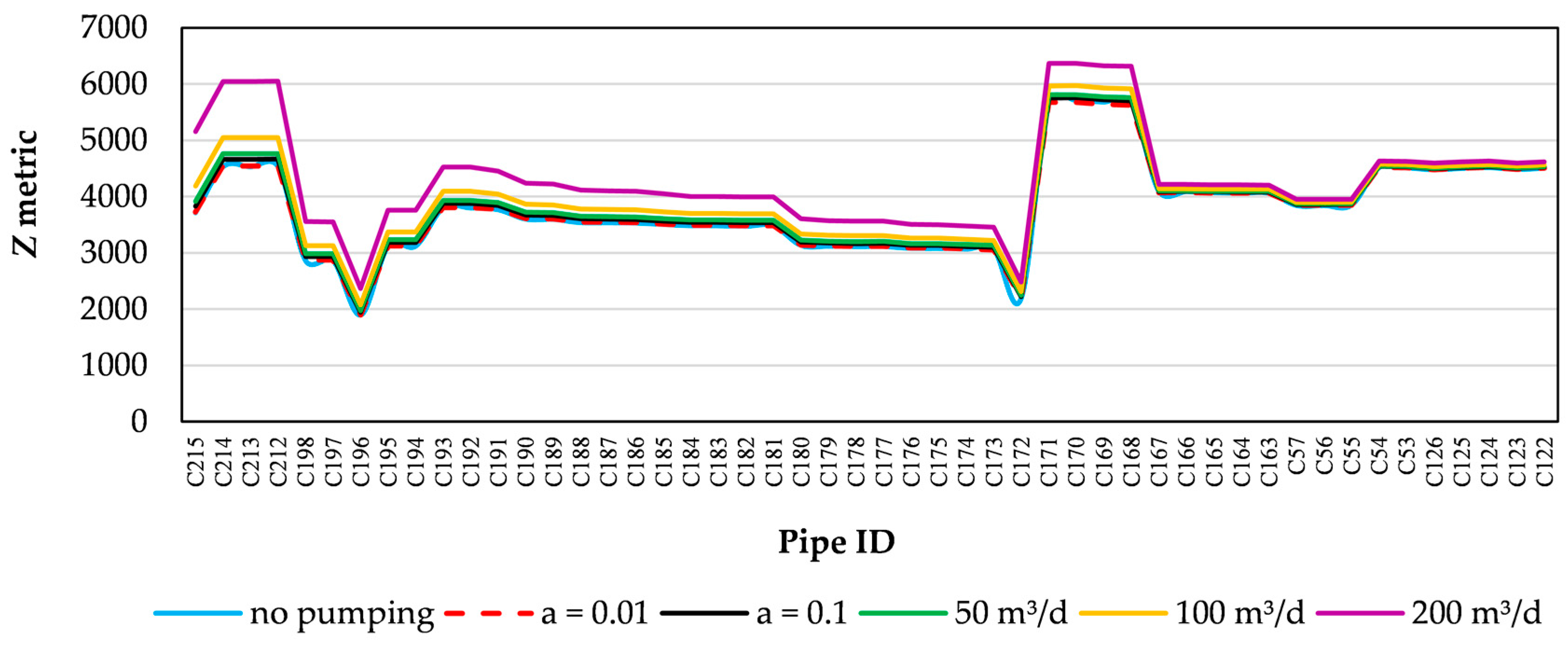
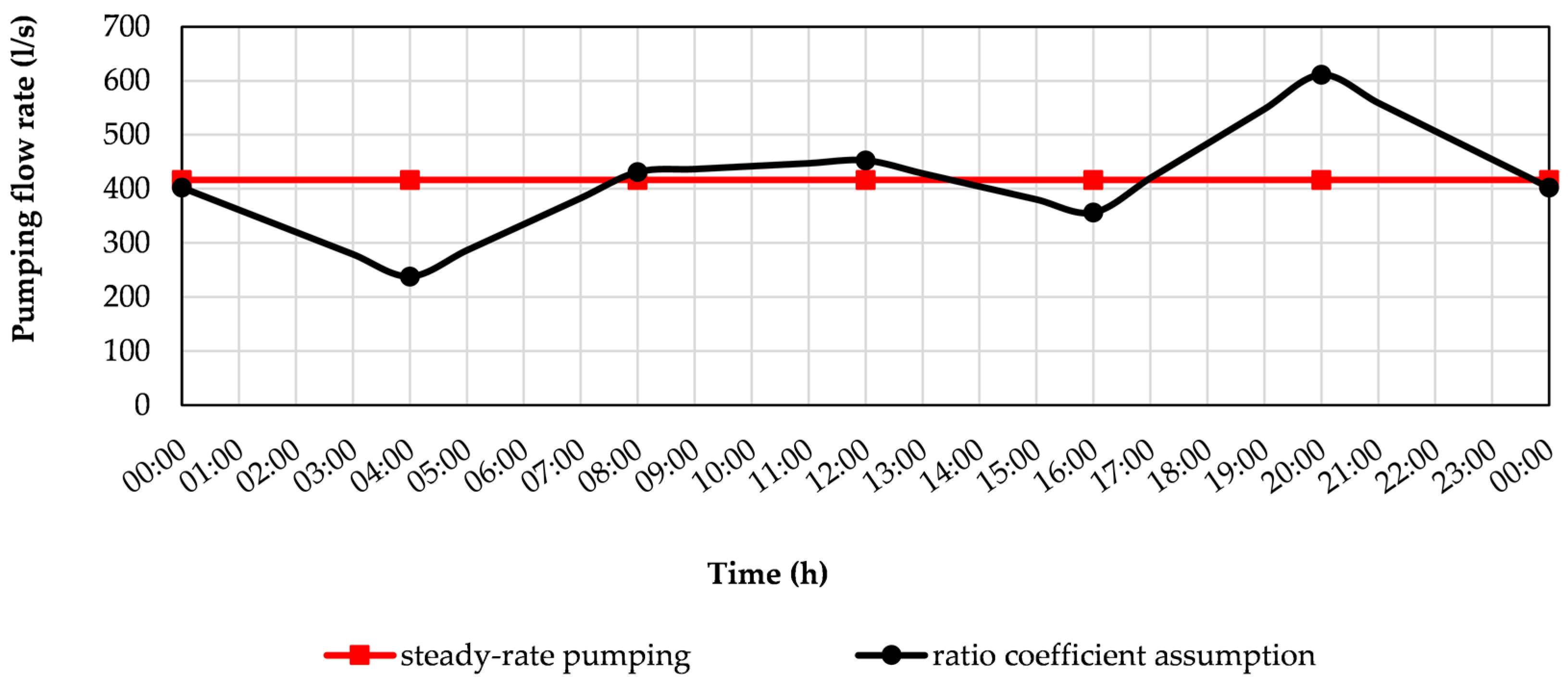
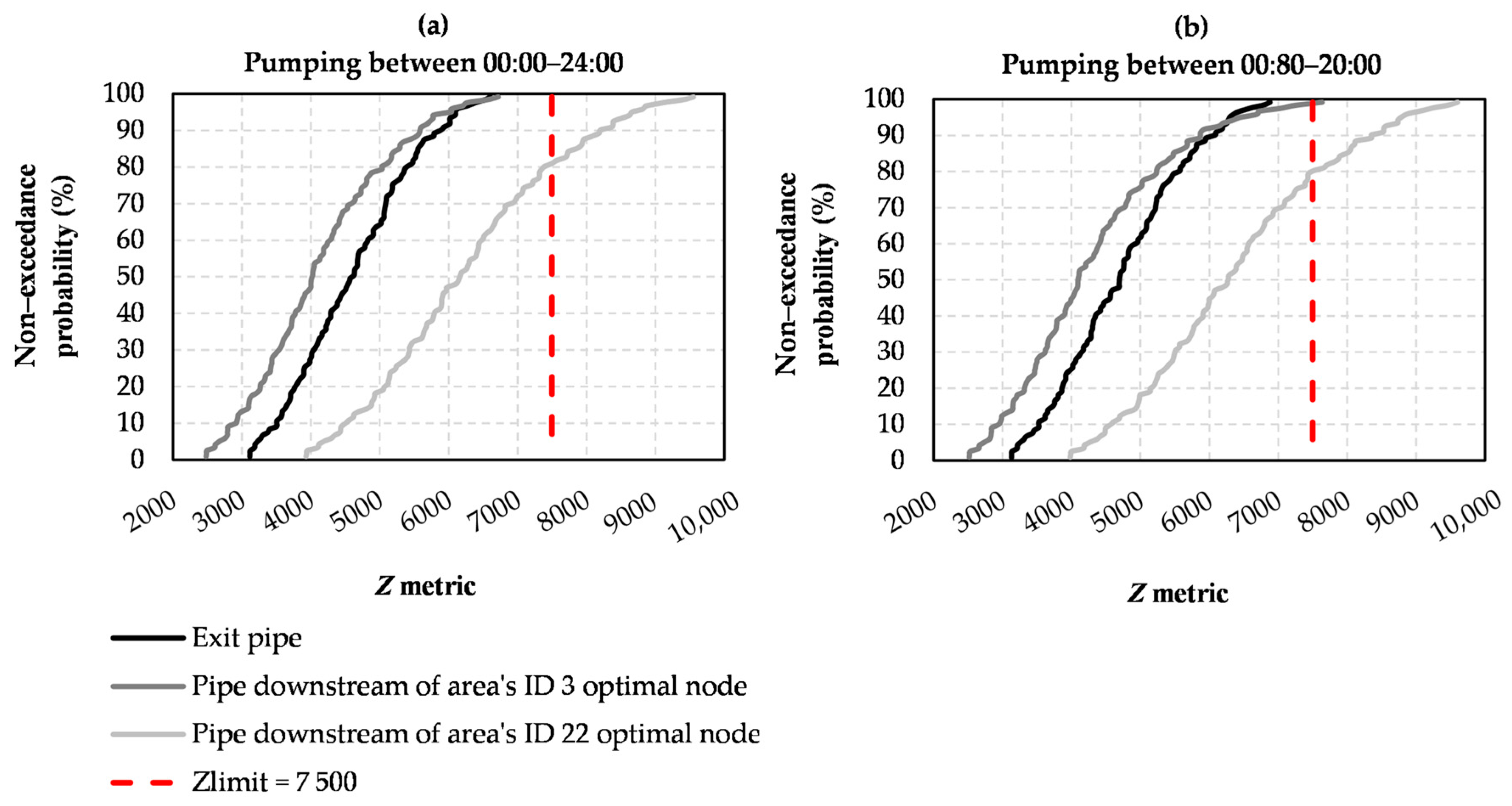
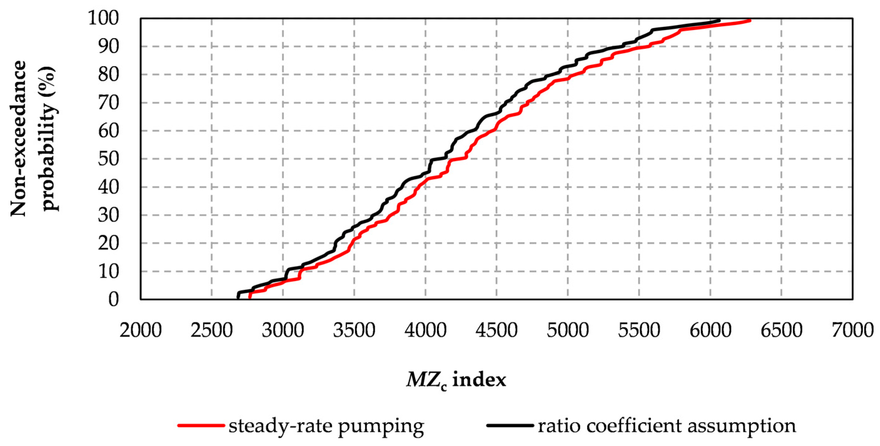
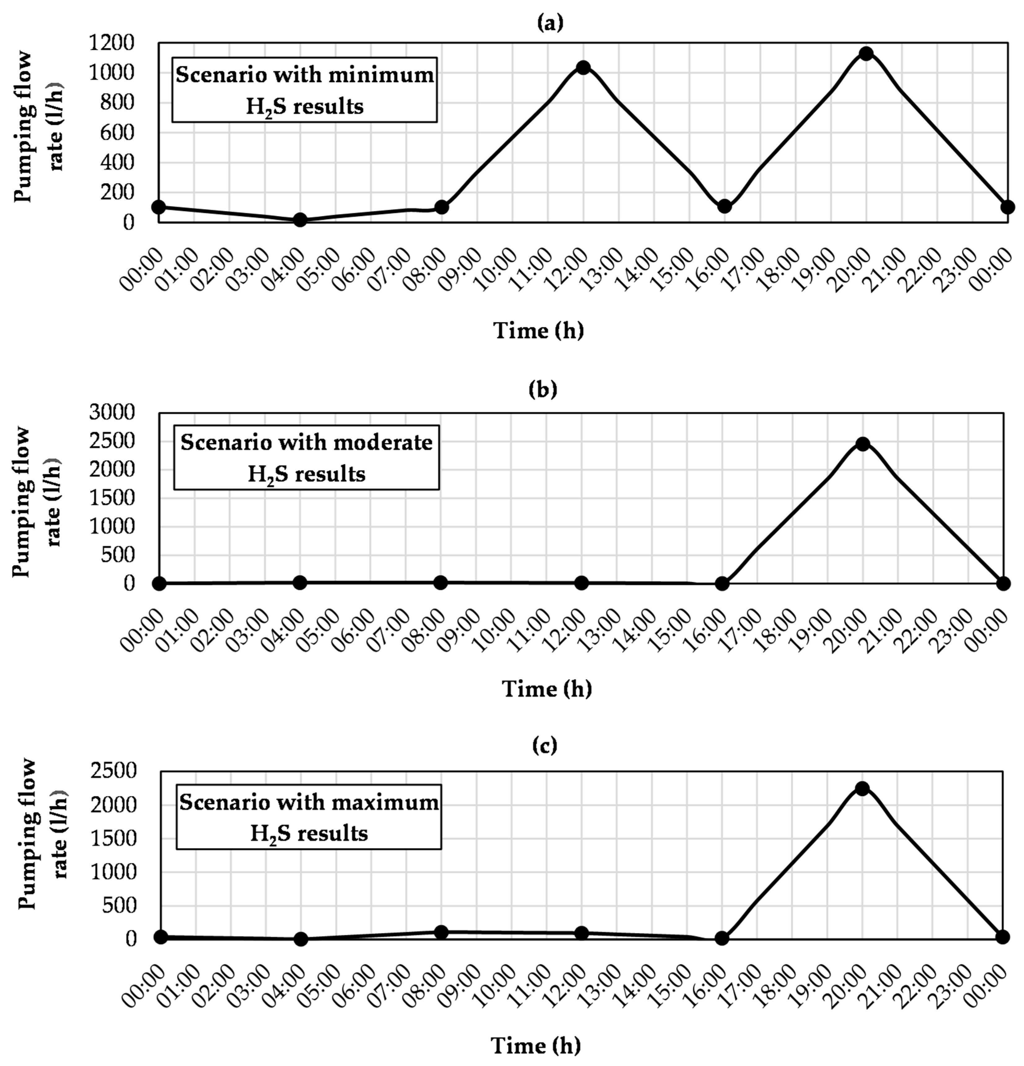
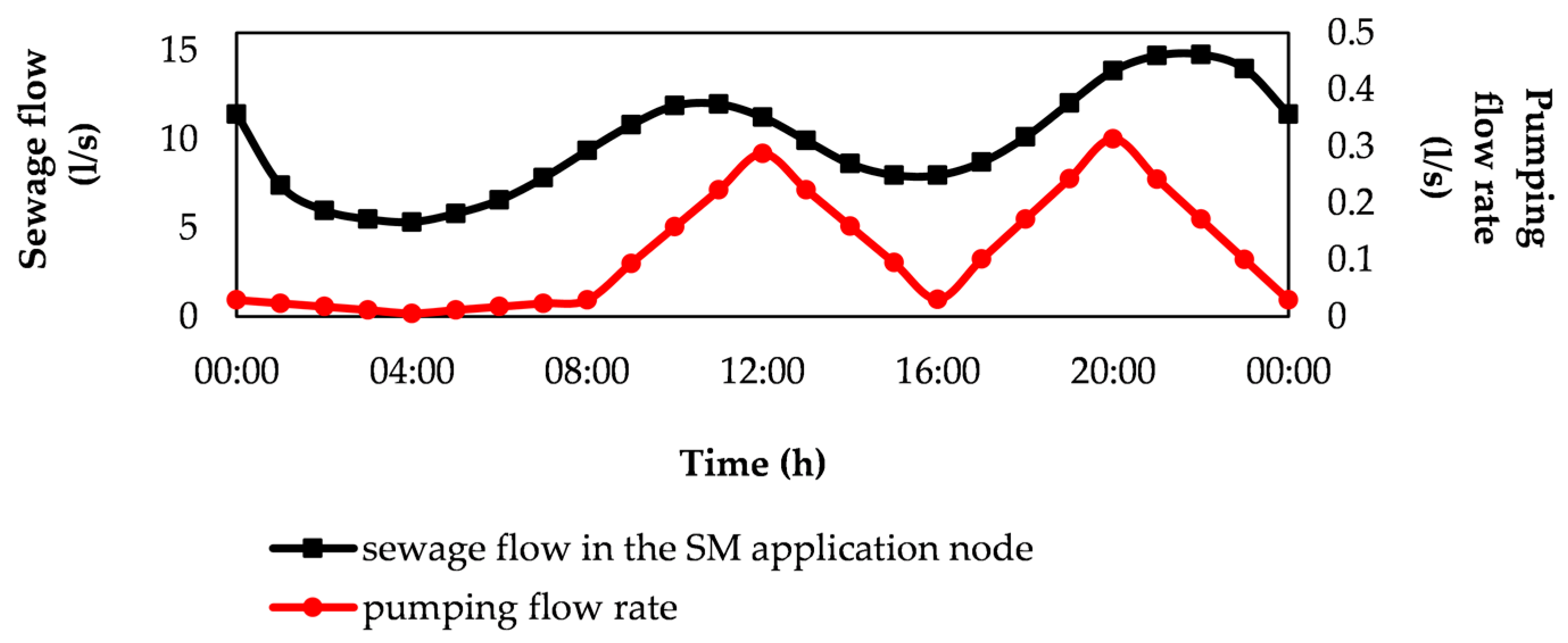
3.3. Optimal Pumping Scheduling

The present study also deals with optimal pumping scheduling when sewer mining is applied. The focus is on minimizing hydrogen sulfide production in the pipe routes from the nodes out of which sewage is pumped to the network’s exit node. In this context, two approaches are considered. As mentioned in Section 2.1, the first approach assumes a ratio between the pumping flow rate and the incoming sewage flow in the sewer mining application node which is expressed through a ratio coefficient, a. The second approach concerns implementing genetic algorithm optimization. In both approaches, it is assumed that no treatment residue returns to the network.

Figure 14 shows the Z metric values across the pipe path from the optimal node of area ID 3 out of which sewage is pumped to the network’s exit node. The results shown in this figure are obtained by simulating a specific loading scenario that provides moderate H₂S production results in the network pipes (more specifically, a loading scenario whose results approach the 50% quantile value of the empiric metric’s values obtained through the N simulations) and concern pumping out of one network node only—the optimal node of area ID 3. Several pumping scenarios are considered for comparison purposes. Two scenarios where the ratio coefficient is employed and set to 0.01 and 0.1 are examined, along with three scenarios where steady pumping rate equal to 50 m³/day, 100 m³/day and 200 m³/day is considered. The results are compared to the non-pumping scenario as well.

It can be stated that when the pumping rate is increased, the Z metric values also increase in all pipes. In the cases where the ratio coefficient is employed, differences are slight because the pumping rate is quite small compared to the sewage flow rate inside the path’s pipes. Nonetheless, in cases of pumping rates higher than 50 m³/day, differences with respect to the Z metric values are considerable. Due to the sewer network’s collective nature, these differences are slight in downstream pipes close to the network’s exit node. It is also observed that the Z ≤ 7500 threshold is not exceeded in any of the pumping scenarios examined.

Furthermore, a comparison between the cases of steady-rate pumping and pumping according to the ratio coefficient assumption is worth making, for the same daily sewage amount pumped out of the network. In this direction, the ratio coefficient is set to a high value (a = 0.5) in order to easily spot the differences between these two cases. The daily sewage amount extracted from the network is then calculated and equally divided between the hours of the day so that the hourly pumping rate values of the steady-rate pumping schedule are obtained.

Figure 15 provides information about H₂S production in the pipe route from the optimal node of area ID 3 to the network’s exit node with respect to the aforementioned cases of pumping. Sewage is pumped out of the optimal node of area ID 3 only. The figure depicts the non-exceedance probability value that corresponds to each MZ_c value regarding the optimal pipe route for the N loading scenarios considered. According to Figure 15, the non-exceedance probability values are higher in the case of pumping when assuming the ratio coefficient. In other words, the probability of H₂S build-up in the optimal path’s pipes is lower in comparison to when steady-rate pumping is applied.

The figures resulting from simulations where sewage is also pumped out of the optimal node of area ID 22 are not presented, as similar observations can be made about them. It should be noted though that extracting sewage out of two different nodes instead of one leads to higher Z metric values, since a wider range of network pipes is affected.

The second approach regarding optimal pumping scheduling includes implementing genetic algorithm optimization. It is assumed that sewage is pumped out of the optimal node of area ID 3 only and that treatment by-products do not return to the network. As described in Section 2.1, the criterion of the optimization is the minimization of hydrogen sulfide production—expressed through the MZ_c index—in the pipe route from the SM application node to the network’s exit node. The algorithm restrictions include the lower and upper bound of the variables (e.g., maximum pump capacity), as well as the linear equalities (e.g., the sum of the amounts of sewage pumped out of the system at each four-hour period must equal to the total sewage amount pumped in a twenty-four-hour period). In the present study, the daily sewage amount pumped out of the network is set to 10 m³. This value is selected in compliance with the SM unit’s capacity of the Athens pilot SM scheme presented in Plevri et al. [45]. Moreover, the pump’s capacity is equal to 5 m³/day. Therefore, the problem’s restrictions are determined according to this information. In addition, the pumping flow rate values are calculated in the cases of steady-rate pumping and of pumping when assuming the ratio coefficient so that the designated daily sewage amount is extracted from the network. These values serve as initial population for the optimization.

Figure 16 shows the pumping flow rate values assigned to the problem’s variables as initial population. Linear interpolation is assumed at the intervals. This figure regards a loading scenario with moderate H₂S production results in the network pipes. Population and generation size are set to 200, so a total of 40,200 iterations are executed. Genetic algorithm optimization is conducted separately for three different loading scenarios of H₂S production in the network pipes (namely, minimum, moderate and maximum H₂S production). The procedure lasts approximately 36–48 h per case.

The optimization results in lower MZ_c values concerning all three loading scenarios examined in comparison to the corresponding values when steady-rate pumping and pumping based on the ratio coefficient assumption are considered. The differences between the results of the three pumping scheduling approaches can be observed in

Table 1. Values of the MZ_c index for three different pumping scheduling approaches and loading scenarios.

Pumping Scheduling Approach	Minimum H2S Production	Moderate H2S Production	Maximum H2S Production
Steady-rate pumping	2487.44	3811.27	5574.80
Assumption of ratio coefficient a	2487.30	3807.18	5570.05
Genetic algorithm optimization	2483.11	3790.36	5534.58

. They are relatively small, yet they would be more significant if the daily sewage amount pumped out of the network increased.

Figure 17 demonstrates the hourly pumping schedules for the three loading scenarios examined which are obtained through genetic algorithm optimization. The pumping flow rates shown in the three panels of Figure 17 are those that resulted at the time of the optimization’s termination—when all iterations have been carried out. Useful conclusions can be drawn by observing them. More specifically, in the scenarios of moderate (Figure 17b) and maximum (Figure 17c) H₂S production results, a tendency towards pumping during the final eight-hour period of the day—between four in the afternoon and midnight—is noted. These pumping schedules are difficult to implement as a general rule due to practical restrictions such as the pump’s capacity and efficiency, as well as the SM unit’s operation hours.

However, Figure 17a, which concerns the scenario of minimum H₂S production results, provides more useful information. The pumping schedule depicted in this panel resembles the flow fluctuations of the hourly pattern in the case of ratio coefficient employment. This resemblance is illustrated in Figure 18. It is therefore concluded that the ratio coefficient assumption can serve as an initial approach in the context of optimal pumping scheduling. Despite that, more thorough analysis is required to find an optimal pumping schedule which is appropriate for a wide range of loading scenarios.

It should be noted that the simulation procedure is very time-consuming with respect to optimization problems. Indeed, the optimization algorithm may need to call the simulation model hundreds or thousands of times so as to accomplish a good solution, depending on each problem’s parameters and restrictions. In order to address this issue, several optimization approaches have been developed aiming to minimize the computational burden, such as parallel computing and surrogate modeling techniques [46,47,48].

4. Discussion

Sewer mining is an innovative decentralized technology that includes sewage treatment aiming at the production of recycled water appropriate for multiple non-potable uses. By extracting sewage (waste) from a sewer network and turning it into recycled water (resource), this technology serves the circular economy purpose. Despite its potential benefits for the environment and ecosystems, its implementation often encounters obstacles. One significant challenge concerns alterations caused in processes related to H₂S build-up inside sewers. Hydrogen sulfide is responsible for odor, corrosion and health-related problems, thus its presence in sewers is undesirable.

The Monte-Carlo method combined with the SWMM model was used in this study focusing on optimal SM unit placement in sewer networks, in terms of minimizing H₂S production. The tool was implemented in a sewer network designed for the town of Kalyvia Thorikou in Greece. A number of model simulations was carried out and H₂S build-up inside sewers was estimated by using the empiric Z metric and the Pomeroy and Parkhurst formula. A multi-criteria optimization with two criteria—the minimization of H₂S production and the maximization of the size of the green area that can possibly benefit from SM implementation—was then conducted to identify potential locations for optimal SM unit placement.

More specifically, two optimal locations for sewer mining implementation were depicted in the Pareto front obtained through the multi-criteria optimization. These are specific nodes included in green areas ID 3 and ID 22 of the case study area. The final selection between the two locations depends on whether the emphasis is put on minimizing H₂S production (area ID 3) or on maximizing the water needs satisfaction (area ID 22). Hydrogen sulfide production was studied more thoroughly in the pipe path from the optimal node of area ID 3 to the network’s exit node. It was concluded that high reliability levels were achieved—as non-exceedance probability values were higher than 90%—and that sulfide concentration did not exceed the predetermined thresholds of 7500 for the empiric Z metric and of 1 mg/L for the total sulfide concentration, according to the Pomeroy and Parkhurst formula. This procedure is considered useful in that it can help find pipes where critical conditions with respect to H₂S production are likely to occur in the future. Therefore, it should be applied before the decision regarding the selection of the location for SM unit placement is made.

After the optimal nodes for sewer mining application were determined, the network’s response in cases where the technology was applied and sewage was extracted from the network was also studied. Several pumping scenarios were considered. The Q[MZ_c]₇₅ values for a reliability level of 75%, as well as the non-exceedance probability of the Z ≤ 7500 threshold, were calculated in the pipes of the pipe paths from the optimal nodes of areas ID 3 and ID 22 to the network’s exit node. The results were compared between the cases of no pumping, of pumping out of one network node (of area ID 3) and of pumping out of two network nodes (of both areas). It was observed that pumping sewage out of the system resulted in lower non-exceedance probabilities and that the more the nodes from which sewage was extracted, the more the conditions related to H₂S production deteriorated, especially close to the extraction point.

Moreover, the study dealt with optimal pumping scheduling with respect to minimizing H₂S production in network pipes downstream of the sewer mining application point. Two different pumping approaches were examined. Firstly, a ratio between the pumping flow rate and the incoming sewage flow in the node out of which sewage was pumped was assumed and expressed through a ratio coefficient. Secondly, a genetic algorithm optimization was carried out separately for three different loading scenarios concerning H₂S production in the network.

The ratio coefficient approach assumed a ratio between the pumping flow rate and the incoming sewage flow in the sewer mining application node which was expressed through a ratio coefficient, a. This coefficient was set to 0.01 and 0.1. The results were compared to the non-pumping scenario and three scenarios where steady pumping rate equal to 50 m³/s, 100 m³/s and 200 m³/s were considered, as well. The comparison concerned a specific loading scenario with moderate H₂S production results in the network pipes, yet useful observations were made from it. It was noted that the higher the pumping rate, the higher the Z metric’s value, especially close to the extraction point. It was also noted that non-exceedance probabilities were lower when assuming the ratio coefficient compared to the steady-rate pumping assumption. Consequently, the ratio coefficient approach can be used as an initial approach in the context of optimal pumping scheduling. Nevertheless, this approach is applicable when the sewage flow and BOD₅ loading follow similar hourly patterns—which is generally the case in urban sewer networks.

The genetic algorithm optimization, carried out for three different loading scenarios with minimum, moderate and maximum H₂S production results in the network pipes, provided some useful results, as well. The hourly pattern of the pumping flow rate resulted from the optimization bore similarities to the corresponding pattern of the incoming sewage flow in the network node from which sewage was extracted. It was therefore concluded that the genetic algorithm optimization approach, combined with the ratio coefficient approach, can be used while seeking an optimal pumping schedule in cases of sewer mining implementation.

5. Conclusions

The tool and methodology presented in this study can be developed and adapted to each case’s needs and restrictions. Improving the modeling procedure by comparing results obtained through the methodology application to real data, is essential to ensure reliability. Unfortunately, no real data are currently available for model validation and this procedure remains a necessary step to be taken in future works. Additionally, more sophisticated approaches and formulas for H₂S build-up estimation may be used, depending on the level of accuracy needed. Nonetheless, computational complexity can hinder the efficiency of the model. To minimize this risk, future works should also deal with balancing computational and modeling performance. Furthermore, it is important to study the effects that the potential return of treatment by-products has on H₂S production inside sewers. In any case, various scenarios, including extreme flow and BOD₅ loading scenarios, ought to be considered so that the corresponding response of the wastewater system is thoroughly examined.

The proposed methodology takes spatial and hydraulic characteristics, as well as sewer network dynamics, into consideration and provides rational and useful results. It is, though, worth noting that multiple factors vary from case to case, such as hourly patterns of sewage flow and pollutant loading, the network layout, characteristics and connections with other networks, treatment facilities or water bodies, as well as restrictions regarding area size, costs and pump operation and capacity). As a consequence, it is difficult to provide a general rule that is applicable for every case. However, the conclusions drawn from the application of the methodology may serve as guidelines for further study concerning the use of upscale sewer mining technologies at a city level.

References

- Angelakis, A.N.; Gikas, P. Water reuse: Overview of current practices and trends in the world with emphasis on eu states. Water Util. J. 2014, 8, 67–78. [Google Scholar]
- Reiter, P. Imperatives for Urban Water Professionals on the Pathway to 2050: Adapting to Rapidly Changing Conditions on a Crowder Planet; International Water Association (IWA): London, UK, 2010; pp. 6–8. [Google Scholar]
- Pereira, L.S.; Cordery, I.; Iacovides, I. Water scarcity concepts. In Coping with Water Scarcity; Springer: Dordrecht, The Netherlands, 2009; pp. 7–24. [Google Scholar]
- Klein, R.J.T.; Midgley, G.F.; Preston, B.L.; Alam, M.; Berkhout, F.G.H.; Dow, K.; Shaw, M.R. Adaptation opportunities, constraints, and limits. In Climate Change 2014: Impacts, Adaptation, and Vulnerability; Cambridge University Press: Cambridge, UK, 2014; pp. 899–943. [Google Scholar]
- Bates, B.C.; Kundzewicz, Z.W.; Wu, S.; Palutikof, J.P.E. Climate Change and Water. Technical Paper of the Intergovernmental Panel on Climate Change; IPCC Secretariat: Geneva, Switzerland, 2008; p. 210. [Google Scholar]
- Anderson, J. The environmental benefits of water recycling and reuse. Water Sci. Technol. 2003, 3, 1–10. [Google Scholar]
- Metcalf & Eddy Inc.; Asano, T.; Burton, F.; Leverenz, H.; Tsuchihashi, R.; Tchobanoglous, G. Water Reuse: Issues, Technologies, and Applications; Mc-Graw Hill: NewYork, NY, USA, 2007; p. 1503. [Google Scholar]
- Crites, R.; Tchobanoglous, G. Small and Decentralized Wastewater Management Systems, 1st ed.; WCB/McGraw-Hill: New York, NY, USA, 1998; p. 1084. [Google Scholar]
- Gikas, P.; Tchobanoglous, G. The role of satellite and decentralized strategies in water resources management. J. Environ. Manag. 2009, 90, 144–152. [Google Scholar] [CrossRef] [PubMed]
- Sharma, A.K.; Tjandraatmadja, G.; Cook, S.; Gardner, T. Decentralised systems—Definition and drivers in the current context. Water Sci. Technol. 2013, 67, 2091–2101. [Google Scholar] [CrossRef] [PubMed]
- EPA. Decentralized Wastewater Treatment: A Sensible Solution. Available online: https://www.epa.gov/sites/production/files/2015-06/documents/mou-intro-paper-081712-pdf-adobe-acrobat-pro.pdf (accessed on 20 January 2018).
- Makropoulos, C.K.; Butler, D. Distributed water infrastructure for sustainable communities. Water Resour. Manag. 2010, 24, 2795–2816. [Google Scholar] [CrossRef]
- Barwon Water. Barwon Water Sewer Mining Guidelines. Available online: https://www.barwonwater.vic.gov.au/vdl/A2413187/Sewer%20Mining%20Guidelines.pdf (accessed on 25 November 2017).
- Marleni, N.; Gray, S.; Sharma, A.; Burn, S.; Muttil, N. Modeling the effects of sewer mining on odour and corrosion in sewer systems. In Proceedings of the 20th International Congress on Modelling and Simulation, Adelaide, Australia, 1–6 December 2013. [Google Scholar]
- Ødegaard, H. Description of an Alternative Urban Water Management System and Its Inherent Technologies; Rapport Nr. 1; Smart Water Cluster: Trondheim, Norway, 2012. [Google Scholar]
- Sydney Water. Sewer Mining: How to Set up a Sewer Mining Scheme. Available online: https://www.sydneywater.com.au/web/groups/publicwebcontent/documents/document/zgrf/mdu0/~edisp/dd_054030.pdf (accessed on 25 November 2017).
- Makropoulos, C.; Rozos, E.; Tsoukalas, I.; Plevri, A.; Karakatsanis, G.; Karagiannidis, L.; Makri, E.; Lioumis, C.; Noutsopoulos, C.; Mamais, D.; et al. Sewer-mining: A water reuse option supporting circular economy, public service provision and entrepreneurship. J. Environ. Manag. 2017. [Google Scholar] [CrossRef] [PubMed]
- Zern, B. From Waste to Resource; WaterHub at Emory University: Atlanta, GA, USA, 2016. [Google Scholar]
- Applied CleanTech. Leading the Sewage Mining Revolution: Presenting a Sustainable, Efficient and Environmentally-Friendly Approach to Wastewater Treatment. Available online: http://www.appliedcleantech.com/files/content/SRS_Brochure.pdf (accessed on 28 November 2017).
- Makropoulos, C.; Tsoukalas, I. Sewer mining for urban re-use enabled by advanced monitoring infrastructure (ami). Presented at the Water Reuse Conference, Barcelona, Spain, 13–14 June 2016. [Google Scholar]
- Haworth, D. A green wicket at the ‘g’—An overview of the mcg water recycling facility. In 76th Annual WIOA Victorian Water Industry Operations Conference and Exhibition Bendigo Exhibition Centre, Bendigo, Australia 3–5 September 2013; Bendigo Exhibition Centre: Bendigo, Australia, 2013; p. 7. [Google Scholar]
- Water Environment Research Foundation (WERF). When to Consider Distributed Systems in an Urban and Suburban Context. Case Study: Pennant Hills Golf Club. Available online: http://www.werf.org/i/c/Decentralizedproject/When_to_Consider_Dis.aspx (accessed on 9 December 2017).
- Dahl, K.; Kirkby, R. Sewer Mining as an Alternative Water Source—The Pennant Hills Experience. Available online: https://www.agcsa.com.au/sites/default/files/uploaded-content/website-content/atm-journal/Water%20Management%20-%20Sewer%20Mining%2C%20the%20Pennant%20Hills%20Experience.pdf (accessed on 8 December 2017).
- McFallan, S.; Logan, I. Barriers and Drivers of New Public-Private Infrastructure: Sewer Mining; CRC Construction Innovation: Brisbane, Australia, 15 July 2008; p. 44. [Google Scholar]
- Rossman, L. Storm Water Management Model User’s Manual Version 5.1; EPA/600/R-14/413 (NTIS EPA/600/R-14/413b); US EPA Office of Research and Development: Washington, DC, USA, 2015; p. 353.
- Rossman, L.; Huber, W. Storm Water Management Model Reference Manual Volume i—Hydrology; EPA/600/R-15/162A; US EPA Office of Research and Development: Washington, DC, USA, 2016; p. 233.
- Marleni, N.; Park, K.; Lee, T.; Navaratna, D.; Shu, L.; Jegatheesan, V.; Pham, N.; Feliciano, A. A methodology for simulating hydrogen sulphide generation in sewer network using epa swmm. Desalin. Water Treat. 2014, 54, 1308–1317. [Google Scholar] [CrossRef]
- Miller, J.E. Basic Concepts of Kinematic-Wave Models; U.S. Geological Survey Professional Paper 1302; United States Department of the Interior: Washington, DC, USA, 1984; p. 36.
- Rossman, L. Storm Water Management Model Quality Assurance Report: Dynamic Wave Flow Routing; EPA/600/R-06/097; U.S. Environmental Protection Agency: Washington, DC, USA, 2006; p. 115.
- Psarrou, E.; Tsoukalas, I.; Makropoulos, C. A decision support tool for optimal placement of sewer mining units: Coupling swmm 5.1 and monte-carlo simulation. In Proceedings of the 15th International Conference on Environmental Science and Technology, Rhodes, Greece, 31 August–2 September 2017. [Google Scholar]
- Tsoukalas, I.K.; Makropoulos, C.K.; Michas, S.N. A monte-carlo based method for the identification of potential sewer mining locations. In Proceedings of the 13th IWA Specialized Conference on Small Water and Wastewater Systems, Athens, Greece, 14–16 September 2016. [Google Scholar]
- Tsoukalas, I.K.; Makropoulos, C.K.; Michas, S.N. Identification of potential sewer mining locations: A monte-carlo based approach. Water Sci. Technol. 2017, 76, 3351–3357. [Google Scholar] [CrossRef] [PubMed]
- Pomeroy, R. The Problem of Hydrogen Sulphide in Sewers, 2nd ed.; Boon, A.G., Ed.; Clay Pipe Development Association: London, UK, 1990; p. 24. [Google Scholar]
- Hvitved-Jacobsen, T.; Vollertsen, J.; Nielsen, A.H. Sewer Processes: Microbial and Chemical Process Engineering of Sewer Networks, 2nd ed.; CRC Press: Boca Raton, FL, USA, 2013; p. 395. [Google Scholar]
- Boon, A.G.; Lister, A.R. Formation of sulphide in rising main sewers and its prevention by injection of oxygen. Prog. Wat. Tech. 1975, 7, 289–300. [Google Scholar]
- Pomeroy, R. Generation and control of sulfide in filled pipes. Sewage Ind. Waste 1959, 31, 1082–1095. [Google Scholar]
- Thistlethwayte, D.K.B. Control of Sulphides in Sewerage Systems; Ann Arbor Science Publishers: Sydney, Australia, 1972; p. 173. [Google Scholar]
- Lahav, O.; Sagiv, A.; Friedler, E. A different approach for predicting H2S (g) emission rates in gravity sewers. Water Res. 2006, 40, 259–266. [Google Scholar] [CrossRef] [PubMed]
- Pomeroy, R.; Parkhurst, J. The forecasting of sulfide build-up rates in sewers. Program. Water Technol. 1977, 9, 621–628. [Google Scholar]
- Yongsiri, C.; Vollertsen, J.; Hvitved-Jacobsen, T. Influence of wastewater constituents on hydrogen sulfide emission in sewer networks. J. Environ. Eng. 2005, 131, 1676–1683. [Google Scholar] [CrossRef]
- Bielecki, R.; Schremmer, H. Biogene Schwefelsäure-Korrosion in Teilgefüllten Abwasserkanälen; Technichen Universität Braunschweig: Braunschweig, Germany, 1987. [Google Scholar]
- Metcalf & Eddy; Tchobanoglous, G. Wastewater Engineering: Collection and Pumping of Wastewater; McGraw-Hill: New York, NY, USA, 1981. [Google Scholar]
- Koutsoyannis, D. Design of Urban Sewer Networks, 4th ed.; National Technical University of Athens: Athens, Greece, 2011; p. 193. [Google Scholar]
- Metcalf & Eddy Inc.; Tchobanoglous, G.; Burton, F.L. Wastewater Engineering: Treatment, Disposal, and Reuse, 2nd ed.; McGraw-Hill: New York, NY, USA, 1979; p. 920. [Google Scholar]
- Plevri, A.; Mamais, D.; Noutsopoulos, C.; Makropoulos, C.; Andreadakis, A.; Rippis, K.; Smeti, E.; Lytras, E.; Lioumis, C. Promoting on-site urban wastewater reuse through mbr-ro treatment. In Proceedings of the 13th IWA Specialized Conference on Small Water and Wastewater Systems, Athens, Greece, 14–16 September 2016. [Google Scholar]
- Tsoukalas, I.; Kossieris, P.; Efstratiadis, A.; Makropoulos, C. Surrogate-enhanced evolutionary annealing simplex algorithm for effective and efficient optimization of water resources problems on a budget. Environ. Modell. Softw. 2016, 77, 122–142. [Google Scholar] [CrossRef]
- Razavi, S.; Tolson, B.A.; Matott, L.S.; Thomson, N.R.; MacLean, A.; Seglenieks, F.R. Reducing the computational cost of automatic calibration through model preemption. Water Resour. Res. 2010, 46, 2387–2392. [Google Scholar] [CrossRef]
- Razavi, S.; Tolson, B.A.; Burn, D.H. Review of surrogate modeling in water resources. Water Resour. Res. 2012, 48. [Google Scholar] [CrossRef]