Abstract
Dissolved oxygen is an essential controlling factor in the performance of facultative and maturation ponds since both take many advantages of algal photosynthetic oxygenation. The rate of this photosynthesis strongly depends on the time during the day and the location in a pond system, whose roles have been overlooked in previous guidelines of pond operation and maintenance (O&M). To elucidate these influences, a linear mixed effect model (LMM) was built on the data collected from three intensive sampling campaigns in a waste stabilization pond in Cuenca, Ecuador. Within two parallel lines of facultative and maturation ponds, nine locations were sampled at two depths in each pond. In general, the output of the mixed model indicated high spatial autocorrelations of data and wide spatiotemporal variations of the oxygen level among and within the ponds. Particularly, different ponds showed different patterns of oxygen dynamics, which were associated with many factors including flow behavior, sludge accumulation, algal distribution, influent fluctuation, and pond function. Moreover, a substantial temporal change in the oxygen level between day and night, from zero to above 20 mg O2·L−1, was observed. Algal photosynthetic activity appeared to be the main reason for these variations in the model, as it was facilitated by intensive solar radiation at high altitude. Since these diurnal and spatial patterns can supply a large amount of useful information on pond performance, insightful recommendations on dissolved oxygen (DO) monitoring and regulations were delivered. More importantly, as a mixed model showed high predictive performance, i.e., high goodness-of-fit (R2 of 0.94), low values of mean absolute error, we recommended this advanced statistical technique as an effective tool for dealing with high autocorrelation of data in pond systems.
1. Introduction
Waste stabilization ponds (WSPs) have increasingly received attention since these shallow lagoons offer a natural biological purification of wastewater with low cost and minimal operation and maintenance requirements [1]. In fact, thousands of its applications currently serve millions of people in many countries across the globe. For example, Dandora WSP in Kenya, the biggest pond treatment system in Africa, serves approximately one million inhabitants or the wastewater from a population of 1.6 million is treated by Western WSP at Werribee in Melbourne, Australia [2]. A distinctive factor of WSPs which allows differentiating them from conventional wastewater treatment plants (WWTPs), is the involvement of algal photosynthesis. During the day, the algal photosynthetic process generates oxygen for aerobic heterotrophs to mineralize organic matters, which, in turn, produce CO2 for the growth of algae [3]. Taking advantage of this natural oxygenation, pond treatment systems reduce operational costs and constrain potential risks from the emission of volatile organic compounds by avoiding mechanical aerations [4]. On the other hand, during the night or under light-limited conditions, such as in cloudy days or at certain water depths, instead of oxygenation, algae respire and thus consume oxygen and release CO2 [3]. In short, the metabolism of algae, which is strongly dependent on spatiotemporal properties and meteorological conditions, can cause a wide variation of the oxygen level in WSPs [5]. Therefore, it is not an easy task for pond engineers to have a proper regulation of oxygen level in which respiratory oxygen required by aerobic bacteria is met by algal photosynthetic oxygen without any additional mechanical aerations.
Although pond technology has been developed over decades, the number of models serving for a better understanding of oxygen dynamics in pond systems remains small. To the authors’ knowledge, there are only two studies, i.e., Kayombo et al. [6] and Banks et al. [7], which applied mathematical models to investigate the oxygen balance in facultative ponds (FPs). Including only algal photosynthesis, the model of Kayombo et al. [6] considered four driving forces of oxygen variation in pond systems, i.e., light intensity, pH, temperature, and CO2. This model suggested that 99% of oxygen production was from the algal photosynthesis while the inflow from primary FP brought 1% left. Banks et al. [7] advanced their model by adding aerobic bacterial assimilation of organic matter whose rate was strongly affected by temperature. Although both studies considered the effect of climatic factors, i.e., light intensity and air temperature, on oxygen balance in pond systems, the interactions between these climatic factors and temporal characteristics were not taken into account. Particularly, even though the hourly variations of light intensity and water temperature were clearly depicted in both studies, only the daily average values were applied in the models instead. In addition, wind mixing as the second mechanism of oxygenation was also neglected in these models. This mass diffusion from the atmosphere was considered as a predominant influencing factor on WSP performance in Li et al. [8].
Oxygen dynamics in pond systems is in terms of not only time but also space. The spatial variation of oxygen is associated with the change in algal community composition and distribution between different ponds and different locations within each individual pond [9]. Pham et al. [10] observed higher values of algal abundance, richness and diversity in maturation ponds (MPs) compared to FPs and lower biovolumes of motile algal species in the inlet compared to the outlet of Ucubamba WSP system in Cuenca (Ecuador). Furthermore, as a result of light attenuation, the algal photosynthesis in FPs can locate only at 20–30 cm from the water surface while that value is around 60 cm for clear and less turbid MPs [11]. In short, these different distributions of algae and its stratification in different depths create a dynamic spatial pattern of dissolved oxygen (DO) in pond systems.
Therefore, our main objective is to investigate the spatial and temporal effects on oxygen dynamic in the WSPs. To this end, the first application of linear mixed effect models (LMMs) in WSPs was implemented. Thanks to its ability to analyze clustered longitudinal data and repeated measures, the spatial and temporal autocorrelations of data can be taken into account [12]. This model was fitted on the data collected from three meticulous sampling campaigns in Ucubamba WSP in Cuenca (Ecuador). Especially noteworthy is that this pond system was located at high altitude, i.e., 2400 m a.s.l., where climatic conditions are relatively severe, i.e., strong solar radiation, low oxygen pressure, and low air temperature with high variation [13]. Therefore, it is expected that the combination effect between the spatiotemporal variations and these extreme meteorological conditions can generate a very dynamic pattern of oxygen level in this WSP. Subsequently, the predictive performance of the mixed model was evaluated via leave-one-out cross validation (LOOCV), through which the detailed description of oxygen dynamics at different depths and daytimes was illustrated. More importantly, considering these findings, together with the fact that DO control in WSPs is overlooked in the previous guidelines of pond operation and maintenance (O&M), insightful recommendations for DO monitoring and control in WSPs were drawn.
2. Materials and Methods
2.1. Study Area
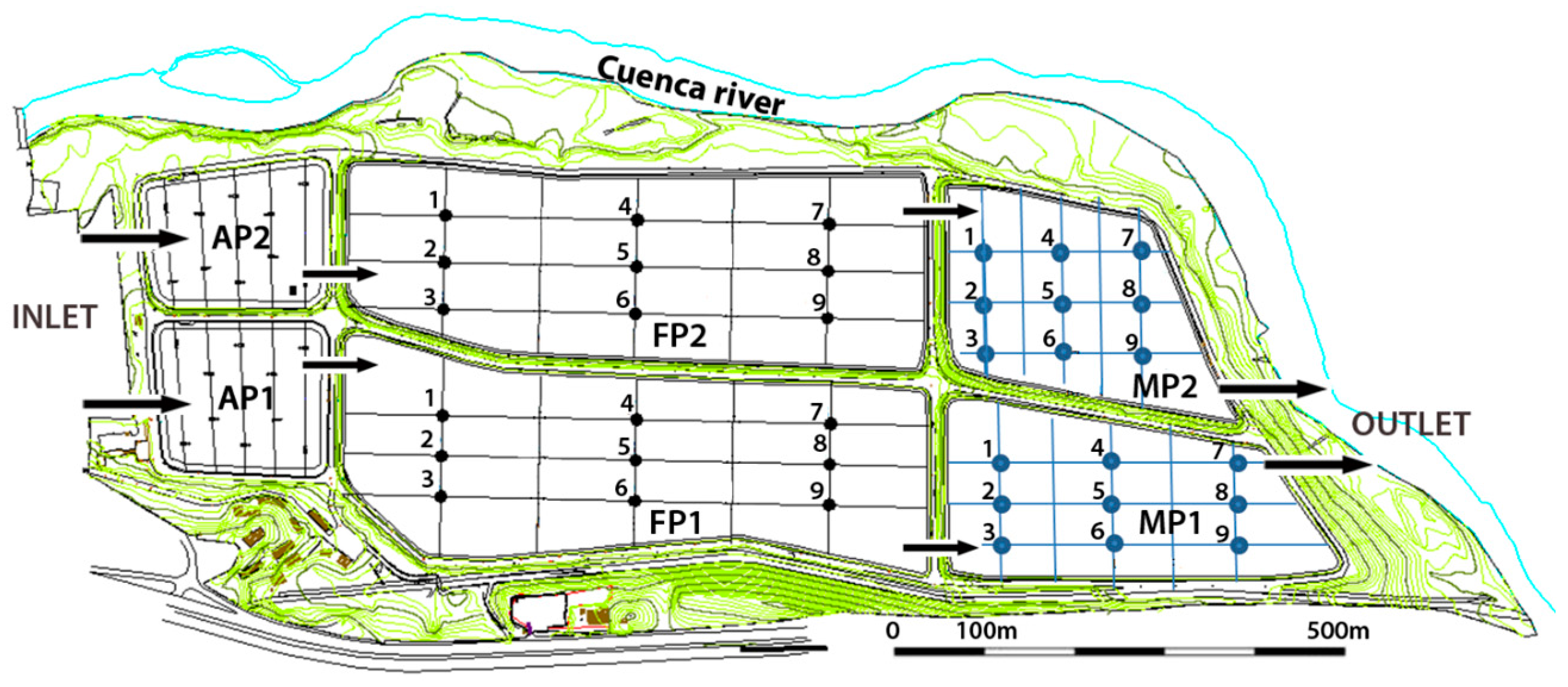
Ucubamba WSP, the biggest wastewater treatment plant in Ecuador, is operated to purify the domestic wastewater of more than 400,000 inhabitants in Cuenca. The pond system is located at the altitude of 2400 m a.s.l. where annual average temperature is 14 °C and average rainfall is about 780 mm per year. Subsequent to pre-treatment steps including screening and grit chamber, the pond system is divided into two identical flow lines, each of which contains an aerated pond (AP), a facultative pond (FP) and a maturation pond (MP) (Figure 1). As a primary treatment, the APs are used as an alternative for anaerobic ponds to remove organic matter and nutrients [14]. These two ponds have a depth of 4.5 m with aerators to supply enough oxygen for oxygenation but not to keep the biomass and influent materials in suspension, hence, organic matters can still be decomposed anaerobically at the bottom of the ponds [15]. With a depth of 1.7 m, FPs decompose the organic matters mainly under aeration conditions as a result of the oxygenation from the microalgal photosynthetic activity. MPs (1.5 m depth) further polish the wastewater, especially in terms of pathogen removal.

Figure 1.
Map of Ucubamba waste stabilization pond (WSP) in Cuenca, Ecuador. Total surface of the WSP is 45 ha in which aerated ponds (APs) occupy 6 ha, facultative ponds (FPs) 26 ha, and the rest is occupied by maturation ponds (MPs) with 12 days of theoretical hydraulic retention time [10,16].
2.2. Sampling Campaigns
Three sampling campaigns were conducted on 25/26 July 2013, 14/15 August 2013 and 26/27 August 2013. Each sampling campaign lasted for two days as the sampling of one line required the period of one day, i.e., from 8:00 a.m. until 6:00 p.m. This course of time covers the whole period of daylight in Cuenca, ensuring the investigation of temporal effects on algal metabolism, hence, on the oxygen variation. Each pond was divided into six sections along the longitudinal direction and four sections breadthways, which created three zones: influent (location 1, 2 and 3), middle (location 4, 5 and 6), and effluent (location 7, 8 and 9) (Figure 1). At two different depths, 30 cm below the water surface and 15 cm above the sediment layer, temperature (°C), pH (−), chlorophyll a (µg Chl a·L−1) and DO (mg O2·L−1) were determined by two manual multi-probes, YSI 6600 V2 and YSI 6920 V1. These probes were carefully calibrated every three days by following their manual in order to ensure their accuracy. At the same time, mixed samples of each zone were analyzed at two different depths for biochemical oxygen demand (BOD5, mg O2·L−1), chemical oxygen demand (COD, mg O2·L−1), total Kjeldahl nitrogen (TKN, mg N·L−1), total phosphorus (TP, mg P·L−1), and total solids (TS, mg·L−1) using American Public Health Association methods [17]. Due to the sludge accumulation, the samples at the bottom of location 1 and 2 of the FPs could not be collected. Meteorological data, including air temperature (°C), solar radiation (W·m−2) and wind speed (m·s−1), were obtained from the meteorological station of CELEC Hidropaute, located 600 m away from the WSP.
2.3. Kruskal–Wallis and Bonferroni Correction
Before applying the mixed model, Kruskal–Wallis tests followed by Bonferroni–Dunn test were applied for multiple comparisons of oxygen between different sampling campaigns, different locations within a pond and among the ponds. Unlike parametric tests, such as one-way ANOVA test, the Kruskal–Wallis test, a non-parametric statistical tool, does not require an assumption of normal distribution of residual. To avoid a type I error, Bonferroni correction is widely applied for correcting the p-values in multiple comparison tests [18]. These tests were carried out using “dunn.test” package [19] in R software Version 3.0.2 [20]. The p-value was considered significant at 0.05/n with n as the number of hypotheses being tested in multiple comparisons.
2.4. Model Selection
One of the main objectives of our research is to investigate the effects of spatiotemporal characteristics and their interactions with meteorological conditions on the variation of oxygen level within the WSP. To this end, LMM, as an advanced technique for statistical modeling, was executed in R [20] using the lme function in the nlme package [21]. Not only taking into account fixed effect as linear regression models, LMM are comprised of both fixed effects and random effects, which can take into account the spatiotemporal autocorrelations of data [22]. The determination of fixed-effect variables was based on the mass balance of oxygen within the ponds. While the main oxygen sources in the WSP system were photosynthesis and the direct exchange of atmospheric oxygen through the air/water interface, oxygen consumption was mostly done by aerobic bacteria for mineralizing organic matter and nitrification process [23]. Particularly in the model, chlorophyll a (µg·L−1) and solar radiation (W·m−2) characterized the photosynthetic activity, while wind speed (m·s−1) and air temperature (°C) represented the oxygen exchange processes. BOD5 and COD represented the bacterial mineralization whilst TKN and TP were nutrients for the growth of algae and bacteria and nitrification process. The spatial and temporal variation of these variables in ponds were also reported in previous studies, e.g., McLaughlin et al. [24] and Guo et al. [25]. Moreover, we modelled the effects of depth and daytime as a logarithm function and a quadratic function, respectively, based on their observed patterns in the studies of Kayombo et al. [6] and Tadesse et al. [26]. Most importantly, the interactions between daytime and the three meteorological parameters were also simulated in the LMM.
Regarding random effect, pond and sampling-campaign parameters were included to account for the spatial and temporal autocorrelation between samples, creating a three-level hierarchical mixed model. More specifically, the unit of analysis, DO concentration (level 1), is nested within pond (level 2), which is in turn nested within sampling campaign (level 3). The detail of this three-level mixed model is demonstrated in Equation (1) and Figure 2:
where:
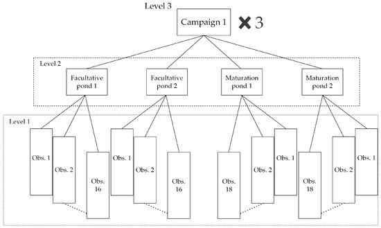
Figure 2.
A path diagram of the three-level hierarchical mixed model. Measurements were taken at nine locations in two different depths within four ponds. Due to the sludge accumulation, the samples at the bottom of location 1 and 2 of the facultative ponds (FPs) could not be collected, which led to 16 observations (Obs.) in the FPs and 18 observations (Obs.) in the maturation ponds in one campaign.
: The concentration of DO of observation i within pond j collected at sampling campaign k. i: 1–16 for the FPs, 1–18 for the MPs, j: 1–4; k: 1–3,
: Fixed effects of the 12 variables,
: Interaction between daytime and the meteorological variables,
: Random effect associated with the intercept for sampling campaign k. ~ N(0,),
: Random effect associated with the intercept for pond j within sampling campaign k. ~ N(0,),
: Residual. ~ N(0,).
To assess the assumptions of the mixed model, such as outliers, multicollinearity, and homogeneity, data exploration was performed following the guidelines of Zuur et al. [27]. Prior to statistical analyses, we assessed the followed assumptions: (1) outliers via the means of Cleveland dotplots (Figure S1), (2) multicollinearity using pairwise scatter-plots comparing the correlation coefficients among covariates (Figure S2), and (3) homogeneity via the residuals of the fitted model (Figures S3 and S4). After removing outliers, the remaining DO concentrations were log10 transformed to stabilize the variance for statistical analyses and then the model was fitted with the dataset. We evaluated the goodness-of-fit of the model via conditional R2 for both fixed and random effects [28]. For residual diagnostics, normality and homogeneity were tested via the QQ plot and residuals vs. fitted values plot (see Figures S5–S7).
2.5. Model Evaluation
The predictive performance of mixed model was evaluated by the mean absolute error (MAE) using leave-one-out cross validation (LOOCV). In particular, the MAE, representing the mean deviation between observed values and predicted ones, was calculated as follows (Equation (2)) [29]:
where Oi is the observed DO in sample i, and Pi is the corresponding prediction based on the mixed model fitted with the full dataset of n samples but without sample i (LOOCV). MAE was chosen over root mean square errors (RMSE) since MAE was concluded as the most natural measure of average error in contrast to the inconsistent functional relationship between RMSE and average error, which might lead to confused interpretations [30,31]. Moreover, the bias and consistency of model prediction were evaluated by regressing observed vs. predicted oxygen concentrations [32].
2.6. Intraclass Correlation Coefficient (ICC)
Autocorrelations in time and space appear when the values of data sampled at the same time and location exhibit more similar patterns than those at different sampling times or further apart. Without considering spatial and temporal autocorrelations, the linear regression model can violate the assumption of independently and identically distributed random variables and draw incorrect conclusions [22]. On the other hand, mixed models with random effects can represent the impact of these autocorrelations by the mean of intraclass correlation coefficient (ICC), which is a measure describing the homogeneity of the observed oxygen concentrations within given clusters, i.e., pond and sampling campaign [33]. ICC is determined as a function of the variance components in a mixed model. For example, sampling-campaign-level intraclass correlation coefficient, ICCsc, was calculated by dividing the variance of the random sampling-campaign effects () by the total random variation. The latter consisted of , the variance of the random effects associated with ponds nested within sampling campaign () and the variance of residual ( (Equation (3)):
The value of ICCsc is high when the total random variation is dominated by , meaning that the oxygen concentrations measured among different sampling campaigns tended to widely vary while these values among different ponds within a sampling campaign are relatively homogenous. The pond correlation coefficient, ICCpond, was calculated as the proportion of the variance of the random effects, , to the total random variation (Equation (4)):
The pond-level ICC is high if there is little variation in the oxygen level within the same pond relative to the total random variation ( is low).
3. Result
3.1. Spatial Variation of Dissolved Oxygen
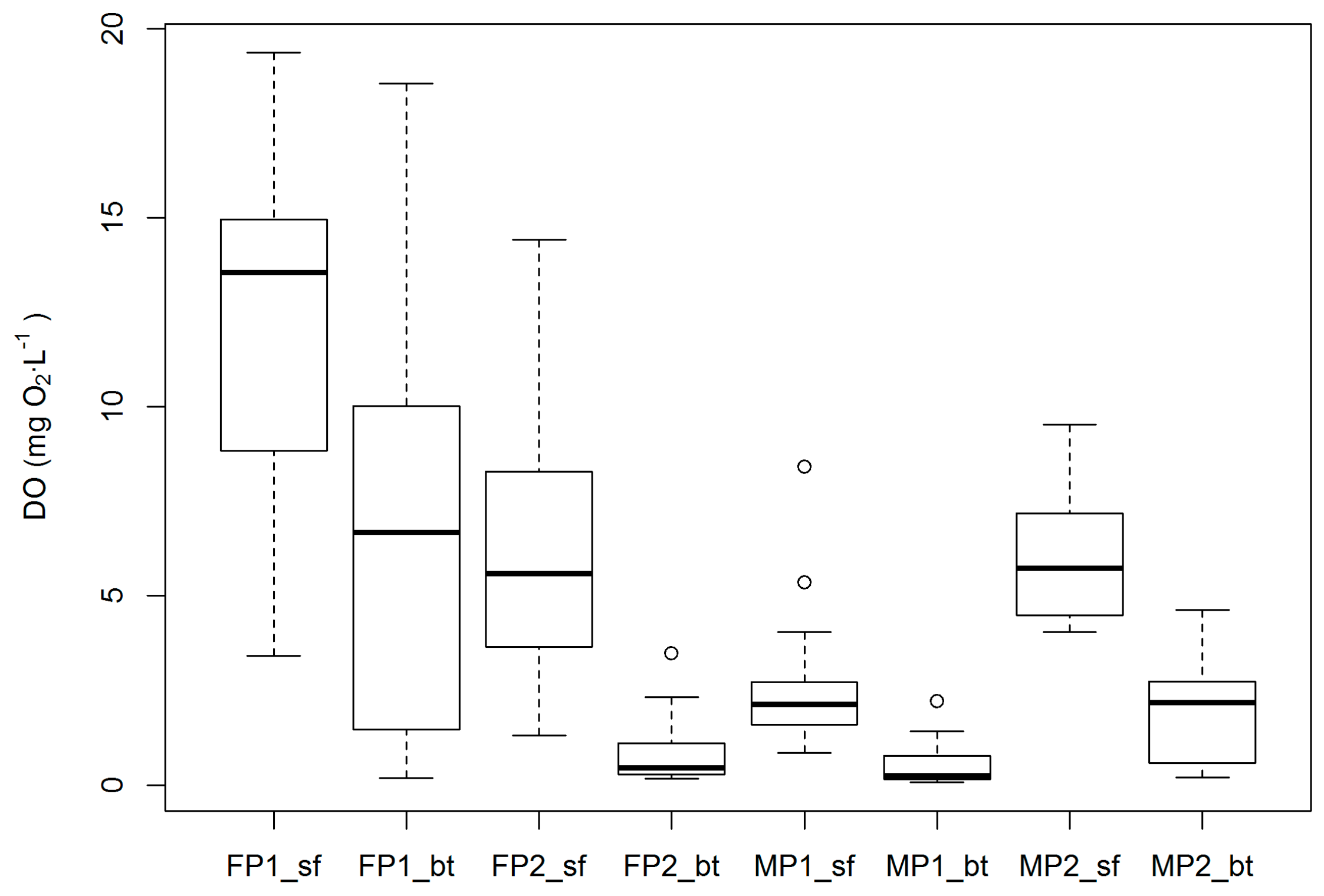
The spatial variations of oxygen level at different ponds and depths are demonstrated in Figure 3. A wide variation of DO was found among four ponds, which corresponded to low p-values of Bonferroni–Dunn tests (p-values < 0.005), except for the comparison between two ponds FP2 and MP2 (p-value = 0.8526). Indeed, there was a different behavior between the two flow lines. Particularly, FP1 contained higher concentrations of DO than its counterpart at the top line, but these values of its consecutive pond (MP1) significantly declined and were lowered in MP2. In fact, from the outlet part of FP1 to MP1 inlet, DO values near the water surface dropped about 70%, i.e., from above 10 mg O2·L−1 to around 3 mg O2·L−1, while the oxygen level remained similar between two ponds in the upper line. This trend also occurred at the bottom layers of the ponds. Between two depths, higher values of both concentration and variation were found close to the surface as being supported by a low p-value of Kruskal–Wallis test (p-value < 0.0001). Much less expected is an extremely high value of oxygen concentration at the bottom of FP1, around 17 mg O2·L−1, which was observed during the last two hours of the afternoon in the first sampling campaign. These extreme values caused very high deviation of the oxygen concentration at the bottom of FP1.
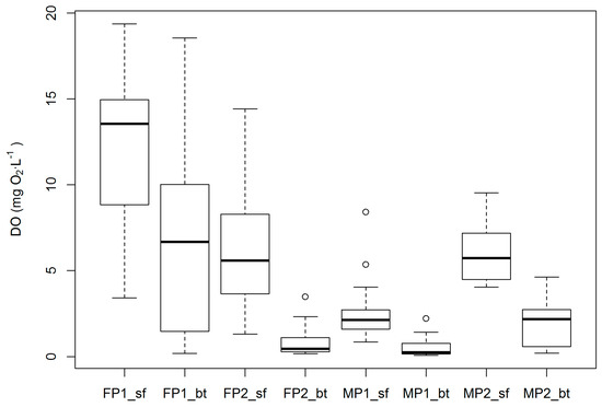
Figure 3.
Variations of oxygen levels between different depths and ponds. Sf: surface; Bt: bottom.
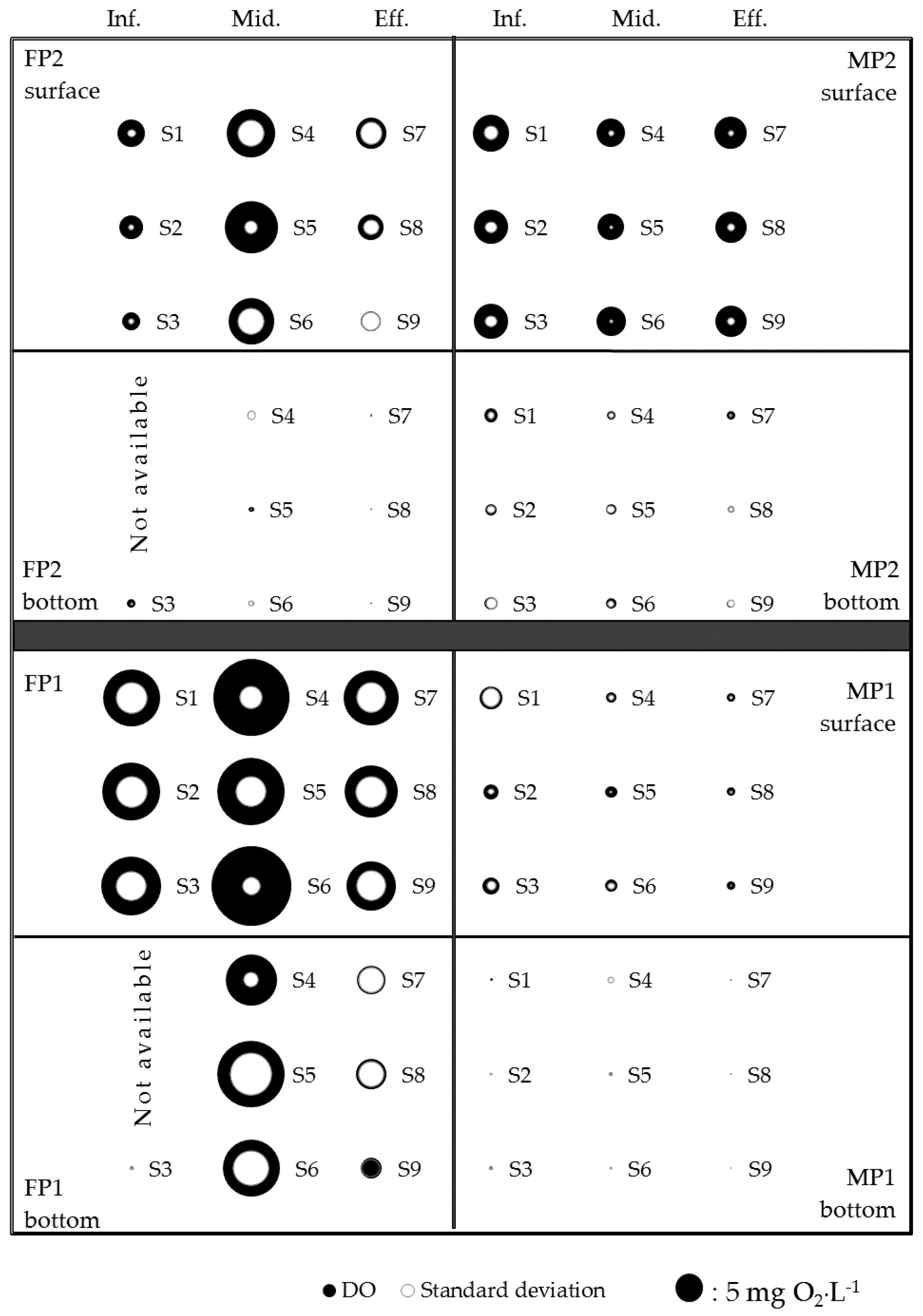
For a further investigation, DO concentrations and variations at the nine locations of each pond in the system are illustrated in Figure 4. Via this bubble plot, the variations of oxygen level within a pond and between two depths are evidently showed. As such, heterogeneous oxygen concentrations were found at different zones across the water surface of the FPs. For example, at the surface of FP1, the highest concentrations were located in the middle area with around 4 mg O2·L−1 higher than those values in the influent and effluent area. Likewise, we also observed higher concentrations and fluctuations at FP2. On the other hand, the oxygen level in the MPs remained homogeneously, around 5 mg O2·L−1 at MP2 surface and 3 mg O2·L−1 at MP1.

Figure 4.
DO concentrations at the nine locations of the ponds. The black circles represent the average values of DO while the white circles represent their variation. The order of the ponds in the graph is analogous to the real system, where the top four boxes correspond to flow line two and the bottom four boxes to flow line one. Due to the sludge accumulation, the values at location 1 and 2 at the bottom of FPs were not available. The area of the black circle in the bottom right corner represents a dissolved oxygen concentration of 5 mg O2·L−1.
3.2. Model Selection
Prior to the statistical modeling, we used pairwise scatter-plots to compare the correlation coefficients among covariates to the threshold of 0.7 as a suitable indicator for the severe distortion effects on model estimation caused by collinearity [34]. The statistical analysis showed that the correlation coefficients among three parameters, i.e., daytime, wind speed, and air temperature, were larger than the threshold (see Figure S2). Hence, we dropped the two meteorological parameters as daytime parameters can be measured with the least effort and cost [27]. Likewise, BOD, COD, and TS also showed high multicolinearity; thus, we removed BOD and TS from the model with the same reason.
In the next step of data exploration, the assumption on homoscedasticity of residual variances was diagnosed via the plots of residuals vs. fitted values and vs. each predictor (see Figures S3 and S4). The residuals vs. fitted plot showed a curvilinear trend, suggesting the heterogeneity of the variance. To deal with this violation, the nlme package provides a standard class of variance function structures for specifying within-group variance models, e.g., fixed weights of a variance covariate (varFixed), constant variance (varIdent), exponential of a variance covariate (varExp). Since varIdent and varFixed were not applicable for a non-linear relationship between residual variance and covariates, varExp function was used as the variance was multiplied by an exponential function of the variance covariate Depth and an unknown parameter δ (Figures S8 and S9) [12].
To build a simple model, backward elimination strategy was applied [33]. Particularly, at first, maximum numbers of fixed effect variables were added in the model, i.e., COD, TKN, TP, pH, chlorophyll a, solar radiation, the log function of depth, the quadratic function of daytime and the interaction between daytime and solar radiation. After that, likelihood ratio tests were employed to test hypotheses about the fixed-effect variables in the LMM based on maximum likelihood estimation [33]. From that, non-significant predictors were identified and removed, i.e., COD (p-value = 0.173), TKN (p-value = 0.138), and TP (p-value = 0.495). The remaining variables, i.e., pH (p-value < 0.0001), chlorophyll a (p-value < 0.0001), solar radiation (p-value = 0.015), depth (p-value = 0.037), daytime (p-value < 0.0001), were kept in the final model as follows (Equation (5)).
where:
~ N(0,) with = 1.85 × 10⁻⁵,
~ N(0,) with = 0.135,
~ N(0,) with = 0.116.
Surprisingly, none of the water-pollutant variables were in the final model, while pH and chlorophyll a appeared as significant predictors. The spatiotemporal effects were proved as daytime and depth were remained in the final model with the interaction between daytime and solar radiation. Regarding the random effects, random intercept for sampling campaign k, ak, is normally distributed with mean 0 and very small variance (1.85 × 10⁻⁵)2 while the random intercept for pond j within sampling campaign k, ajk is normally distributed with mean 0 and much higher variance 0.1352. From these variances, intraclass correlation coefficients were calculated, resulting in ICCsc of 1.08 × 10⁻⁸ and ICCpond of 0.58. Concerning the goodness-of-fit of the model, we obtained very high conditionals R2 of 0.94, which suggested both fixed and random effect variables providing considerable potential in predicting the oxygen level within the pond system.
3.3. Model Evaluation
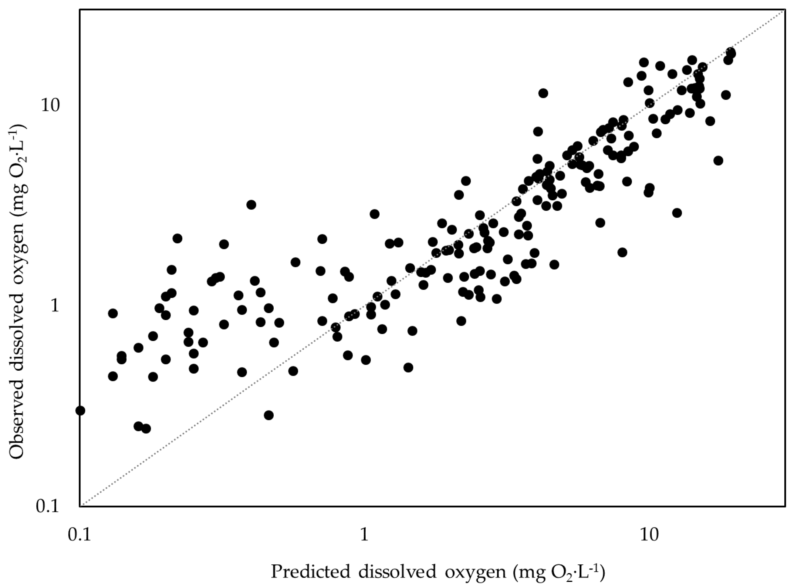
To assess the predictive performance of the model, a scatter plot of observed vs. predicted values was drawn (see Figure 5). Testing of the model predictions against observed data demonstrated that the model was capable of capturing the variation of oxygen level within different ponds. Indeed, except for the lowest concentrations of oxygen being slightly underestimated, the model predictions deviated less than an order of magnitude, inferring high model accuracy and consistency.

Figure 5.
Observed vs. predicted regression scatter plots derived from the mixed model. The dot line is a 1:1 line.
Figure 6 showed the MAE values between predicted and observed oxygen concentrations at two different depths in each individual pond and the whole system. Generally, relatively low MAEs indicated the fairly high accuracy of the mixed model. Apart from the high MAEs of FP1, this measure of error was lower than 1.3 mg O2·L−1 in the other ponds. In fact, 26 out of 30 highest values of MAE were from the samples collected at FP1. The other four values belonged to the samples at MP2, causing this pond having the second highest values of MAE. It is noteworthy that both of these ponds had the highest fluctuation of oxygen level at the two depths.
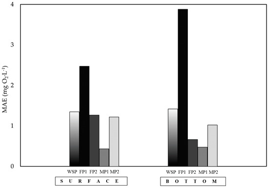
Figure 6.
Summary of the forecast error measure of the mixed model. MAEs were calculated between predicted and observed oxygen concentrations at two different depths in each individual pond and the whole system.
3.4. Diurnal Dissolved Oxygen Profile
The hourly variation of oxygen concentration was illustrated in Figure 7. Particularly, the graph depicted the mean observed and predicted oxygen concentrations with their equivalent values of MAE. These values were averaged over four ponds at two different depths. At the surface, the observed oxygen concentration gradually increased from 9:00 a.m. onwards and reached its peak, around 9 mg O2·L−1, from noon to 5:00 p.m. On the other hand, the increasing trend started later at the bottom from around 12:00 p.m. and then the oxygen level surprisingly boosted to the same concentration at the surface layer during the last two hours. In fact, during this time of the first sampling campaign in FP1, a heavy rain was recorded, causing abnormal oxygen concentrations at the bottom layers, up to 16 mg O2·L−1. Comparing to the collected data, the mixed model was able to describe relatively precisely the diurnal oxygen variation, especially at the surface where the average MAE was only 0.80 mg O2·L−1. Similarly, except for the last two hours when the oxygen level was greatly underestimated, the average MAE values for the prediction of the samples at the bottom layers were very low, i.e., 0.52 mg O2·L−1.
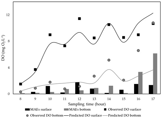
Figure 7.
Predicted and observed diurnal oxygen profile with MAE values at two different depths in each hour of sampling campaign. The dots and lines represent observed and predicted oxygen concentrations, respectively, while the bars represent their equivalent MAE values.
3.5. Vertical Dissolved Oxygen Profile
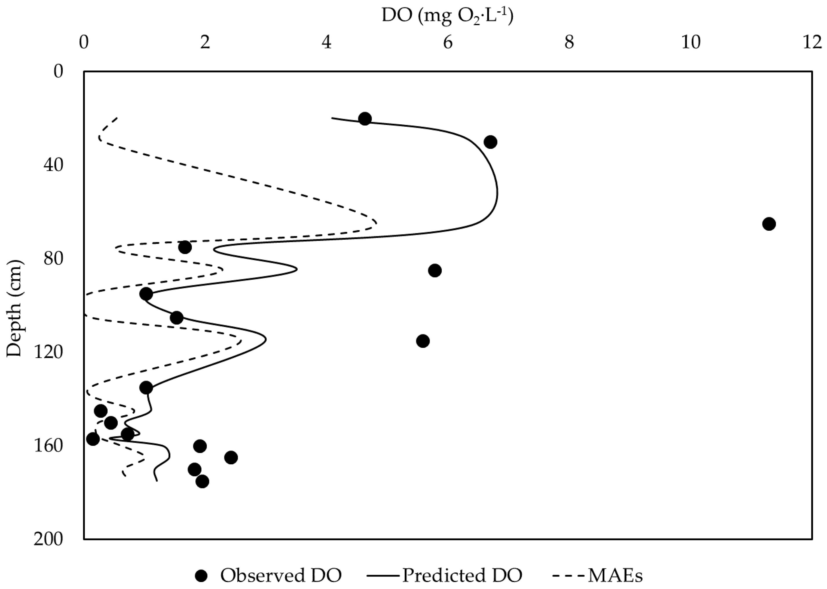
Figure 8 demonstrated the vertical dissolved oxygen profile of the pond system, in which predicted and observed oxygen concentrations with the corresponding values of MAE were averaged over four ponds at different depths. As showed in the figure, the mixed model predicted the vertical pattern of oxygen reasonably well as it captured the sudden drop of oxygen level from epilimnion to hypolimnion layer, which can be a consequence of algal stratification due to light limitation [5]. There were three abnormally high oxygen concentrations at depths 65, 85, and 115 cm, which were recorded at FP1 in the heavy-rain conditions, causing high MAEs of around 3 mg O2·L−1.
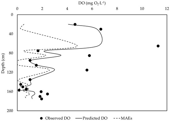
Figure 8.
Predicted and observed DO profile along the pond depth with the values of MAE. The dots and the continuous line represent observed and predicted oxygen concentrations, respectively, while the dashed line represents their equivalent MAE values.
4. Discussion
4.1. Spatiotemporal Influences on the Oxygen Dynamic
Spatiotemporal autocorrelations can be seen as both an opportunity and a challenge as it can provide useful information for inference of process from their patterns [22]. In fact, to account for these autocorrelations, we implemented the first application of mixed model in WSPs, which underlined the variations of oxygen concentrations with respect to time, and space in a high-altitude WSP. The LMM (Equation (5)) showed the negative impact of depth (regression coefficient = −0.59) and the diurnal effects with the shape of a downward opening parabola as the coefficient of daytime2 is −0.02. These results agreed with the observed data from the three sampling campaigns as shown in Figure 7 and Figure 8 as well as the high value of conditional R2 of 0.94. Interestingly, none of the water-pollutant variables, i.e., COD, TKN, and TP, was included as the fixed-effect variables in the final model. The reason could be because of high oxygen concentrations as a result of the enhanced algal photosynthesis, which was accelerated by strong solar radiation in this meridional high-altitude WSP system. Compared to this high production of DO, the amount of oxygen, which was consumed for bacterial mineralization and nitrification process, appeared to be inconsiderable. Indeed, the remaining fixed-effect variables are related to only the algal photosynthesis and their positive coefficients, i.e., pH (0.27), chlorophyll a (0.0009), and solar radiation (0.007), also support the substantial influence of algal photosynthesis on the spatiotemporal variations of oxygen concentration.
Moreover, the spatiotemporal variations of DO were highlighted via the random effects. In particular, the very low variance of the random sampling-campaign effects () leading to almost zero ICCsc suggested that there was nearly no dissimilarity in the oxygen variation among the three sampling campaigns. The reason of this similarity can be explained by the fact that the sampling campaigns were conducted within one dry season of Ecuador when a very widely fluctuated oxygen level can be observed over the course of one day as showed in Figure 7. In Cuenca, daylight lasted from 6:00 a.m. to 6:00 p.m. with peak of solar radiation between 1:00 p.m. and 3:00 p.m. promoting the maximum rate of algal photosynthesis [35]. During this peak period, an extremely high oxygen level was recorded, i.e., more than 20 mg O2·L−1 in our sampling campaigns and up to 39 mg O2·L−1 in the sampling campaign of Alvarado [35] in this pond system. These abnormally high oxygen levels can be induced by vast light intensity at high altitude, up to 1500 W·m−2, and high algal biomass above 420 µg Chl a·L−1 near the surface of the FPs. This high algal biomass can be a result of intensive solar radiation at high altitude. In fact, in a WSP located at an altitude of 2675 m in Mexico, Pearson et al. [36] also found extremely high levels of chlorophyll a, up to 1500 µg Chl a·L−1. This algal overgrowth can generate a supersaturated DO condition during the day, but, on the other hand, depletes the oxygen level due to their respiration during the night [37]. As such, a vast fluctuation of the pond performance can be found between early morning and mid-afternoon in a high-altitude WSP.
Contrast to the very low ICCsc, the relatively high value of ICCpond of 0.58 suggests that both the variance of the random effects associated among the ponds () and the variation of the oxygen concentration within a pond () were considerable. Indeed, the variations associated among the ponds derived from the difference in pond performance across the two flow lines. More specifically, FP1 received around 20% higher pollutant loadings than FP2, especially organic matter. In fact, their average surface organic loadings were up to 250 and 185 kg·ha−1·day−1, respectively, while the recommended limitations were 240 kg·ha−1·day−1 for WSPs at tropical and subtropical regions and only 200 kg·ha−1·day−1 for WSPs at altitudes above 2400 m a.s.l. [13,38]. These high loadings were associated with the sludge accumulation, which was also the reason of unavailable data at the bottom of location 1 and 2 in FPs. According to the study of Alvarado et al. [39] in this pond system, the sludge volume of the FPs reached up to 34% of the pond volume, which substantially reduced its active volume.
Regarding the variation within a pond, in contrast to a relatively homogeneity of oxygen level in the MPs, higher concentrations were found at the central area of the FPs. This difference can be caused by the fact that the central area of the FPs had less sludge accumulation and flow turbulence, which promoted high density of algae located at this region [39]. On the other hand, the bathymetries in the study of Alvarado et al. [16] on these MPs showed only a slight sludge layer growth in the maturation ponds that can be assumed negligible regarding the pond hydraulics.
4.2. Model Evaluation
The mixed model proved its ability to capture the very dynamic variation of oxygen level in a high-altitude pond system. This is supported by very high goodness-of-fit, a fair agreement between predicted and observed values (Figure 7 and Figure 8), and low values of MAEs, which were normally smaller than 10% of the predicted data, except for the abnormally high DO observed in FP1. This abnormality was generated due to the heavy rain with high wind speed, above 5 m·s−1, leading to high turbulent flow that homogenized the water column, creating very high concentrations of DO, up to 16 mg O2·L−1. These values caused poor predictive performance of the mixed model during the last two hours of the first sampling campaign. This underestimation can be explained by the sensitivity of mixed models to abnormal observations [40] and the fact that the three sampling campaigns were conducted within one dry season of Ecuador. As the photosynthetic activity of algae changes in response to the seasonal changes in environmental conditions [24,41], there is a need for additional sampling campaigns in the rainy season. From that, the interpolation of this mixed model can be reliably performed within a larger range of observation.
Concerning the model applicability, a question should be raised, related to the usefulness of this mixed model in terms of predicting oxygen concentrations compared to previous mechanistic models. Firstly, when encountering with the complex interactions of multifaceted factors in ecological systems, a statistical model can be preferred over a mechanistic model due to its simplicity [42]. Especially noteworthy is that the WSP system as an open natural system should be considered as a complicated assemblage of different processes and inputs, hence, its mechanistic models are nearly always overparameterized [43]. In fact, to simplify the models, some important processes were neglected in Kayombo, Mbwette, Mayo, Katima and Jorgensen [6] and Banks, Koloskov, Lock and Heaven [7], e.g., nutrient uptake of bacteria and algae, nitrification/denitrification, and air/water exchange. More importantly, numerous parameters applied in mechanistic models have been taken from different systems and model assumptions based on external characteristics might have to be applied. This approach of artificially assigning values to parameters can lead to biased results, which significantly deviates from real outputs [38]. Indeed, several simplifying assumptions along with geometric approximations caused the disagreements between computational fluid dynamics (CFD) model outputs and experimental results in the research of Alvarado, Sanchez, Durazno, Vesvikar and Nopens [39]. Finally, the large number of experimental data needed for the validation of mechanistic model is another major constraint.
4.3. Insights for Oxygen Regulation in WSPs
According to previous guidelines of Pearson et al. [44], and Mara and Pearson [45], DO was identified as an additional parameter for effluent quality monitoring and evaluation of pond performance, as it is determined not necessary to monitor this extra parameter for routine monitoring and evaluation. Nevertheless, this is totally not the case in conventional biological WWTPs using activated sludge. Oxygen levels are considered a key parameter in the operation of such a plant and DO control is of primary importance in activated sludge processes [46]. Particularly, DO concentration should be sufficient for aerobic microorganisms to degrade organic matters and convert ammonium to nitrate, yet it is not excessive to deteriorate the sludge formation, which can lead to the problem of sludge settleability. In addition, as air supply accounts for the largest portion of the operational budget of these plants, proper DO control can save enormous energy costs compared to uncontrolled systems [47]. In fact, to optimize the operation of WWTPs, DO control via aeration is one of a very limited number of manipulatable variables so that has been the subject of extensive research since the 1970s [48]. In contrast to this maturity, the omission of DO control in WSPs can be a neglected reason causing many common problems in pond operations, such as organic overloading, odor problems, and algal overgrowth. This lack of proper control and poor operation was reported as one of the main reasons for the under-performance of eight high-altitude WSP systems in Mexico [49]. Given these points, pond engineers need a more advanced strategy for O&M in general and DO control in particular. To do so in conventional WWTPs, instrumentation, control, and automation (ICA) as an advanced tool for system control has been long developed and is now well-recognized as an integrated part of plant operation while this technology has been very new in pond operation up to now [48]. This limitation is because, for small-scale ponds, the O&M tends to be neglected due to financial reasons while, in large-scale systems, pond engineers are still more comfortable with the traditional procedures [5]. However, since effluent discharge standards become increasingly stricter and levy charges for plant performance failures can sharply increase the O&M costs, advanced control appears to be a more economic and reliable method. As such, we propose following practical recommendations on DO monitoring and regulation in WSPs, based on ICA technology and the findings from our research.
Firstly, the flow behavior of a pond should be taken into account in the DO control as it can considerably affect oxygen variations. While homogenous oxygen levels are normally observed in completely mixed systems, the DO profile in plug-flow-like ponds, which reflects oxygen uptake rate (OUR), can vary greatly along the systems [50]. Different from activated sludge systems where these two ideal regimes are commonly applied, the mixing behavior in WSPs is more complicated as being affected by many factors, such as inlet/outlet configurations, wind, sludge accumulation, and baffles [51]. As such, in order to evaluate DO profile and flow performance, we suggest that the locations in the grid scheme in Figure 1, which cover the three essential areas of a pond, i.e., influent, middle, and effluent, are needed to be sampled. From that, we can identify the flow stratification and recognize dead spots, stagnant areas, and possible sludge accumulation as it was the influent area in our case. It is noteworthy that baffled ponds, where the hydraulic regime is similar to the ideal plug flow, can offer more flexibility for DO control but also greater challenges [52]. In plug-flow systems, different DO set-points can be chosen along the reactors, providing independent zones that can be used for different purposes, such as aerobic zones for nitrification and anoxic zones for denitrification. Such a configuration leads to a more complex control system, which needs to include ammonia and nitrate sensors like in Kallby WWTP (Sweden), which has ten zones with a pre-denitrification configuration [47]. This potentiality in baffled ponds to increase the nutrient removal can be exploited via optimal control and design to setup the most appropriate measurements and their corresponding set-points. Such a study is surely guaranteed, but still needs to be done.
Secondly, pond engineers also need to evaluate the vertical DO profile which is a result of algal stratification reflecting light availability along the water depth. Generally, light and photosynthetic activity can extend down to the bottom of shallow MPs where clean and less turbid water is located, while, with higher concentration of suspended solids, this extension for FPs is only 20 to 30 cm [5]. This light attenuation can be very important for pond performance. The location of the sudden drop of oxygen defines the volume of anoxic and anaerobic area in FPs (see Figure 8). Vigorous mixing can carry oxygenated water from upper aerobic layers to the bottom area, which limits the extent of methane fermentation, leading to acidic conditions and odor release [53]. This common problem of shallow FPs occurred during the last two hours in the first sampling campaign when the heavy rain and strong wind homogenized the oxygen level within the water column in FP1 (see Figure 7). The occurrence of such a disturbance is the major incentive of system control. Naturally, WSPs are relatively resilient to disturbances as a result of large volume and thus high HRT. However, besides encountering a large variation of wastewater influent regarding both its composition and flow rates, WSPs, especially the systems at high altitude, also have to deal with the hourly, daily and seasonal changes in climatic conditions. A traditional way of tackling this issue was to build a larger volume as it was a suggestion of Juanico et al. [13] for high-altitude WSPs. Compared to ICA technology, it is not the best economic solution, as overly conservative designs can inflate capital and O&M costs of the plants and is not an optimal choice for pond upgrading [52]. Regarding MPs, two key mechanisms of disinfection process involve photo-oxidation, which essentially relies on the presence of DO and pH [54]. Indeed, it was concluded in Curtis et al. [55] and Dixo et al. [56] that sunlight-mediated disinfection can only have a considerable impact on fecal coliforms in the case of high DO and pH present. Interestingly, high algal biomass generates high DO and pH, and reduces the light penetration in the ponds since algae contain large amounts of pigments that can block sunlight [57]. Hence, in MPs with low concentrations of other light absorbers, such as gilvin and tripton, the information from the DO profile showing the algal distribution and light penetration can facilitate the evaluation of pond disinfection efficiency.
Moreover, as 80% of the oxygen source in ponds originates from algal photosynthesis, pond engineers should keep in mind its diurnal variation. The period of daylight should be recorded, as solar radiation is the main energy provider for the ponds. It is also recommended that the sample of DO should be collected periodically at a minimum of three moments in a day, i.e., sunrise, noon, and sunset. Extra care should be given in high-altitude pond systems since high light intensity promoting algal overgrowth can generate supersaturation of oxygen during daylight but drain out oxygen when the light diminishes. This can lead to overload and violate the discharge permit; hence, extra aeration may be needed during the night. Furthermore, as not only algal photosynthetic activities but also other characteristics of ponds, such as nutrients, bacterial levels, and dissolved organic matter changes seasonally [24,25], it is advised that the oxygen profile should be recorded and compared between different seasons during a year for an accurate depiction of pond performance.
5. Conclusions
The first application of a linear mixed effect model highlighted the spatiotemporal variations of oxygen level in WSPs, which were enhanced by severe meteorological conditions at high altitude in this study. Particularly, a substantial diurnal variation was observed from zero to above 20 mg O2·L−1, which can be a result of algal overgrowth as it was expedited by the intensive solar radiation at 2400 m a.s.l. This algal bloom generated supersaturation of oxygen during the day but drained out oxygen via their respiration during the night. The critical role of algae in the oxygen temporal dynamics was also emphasized in the final model, as all the remaining fixed-effect variables were associated with the algal photosynthesis. Despite being designed in the two parallel flow lines, different ponds exhibited different spatial patterns of oxygen dynamics as a result of numerous factors, such as flow behavior, sludge accumulation, algal distribution, influent fluctuation, and pond function. In the mixed model, this spatial variation was indicated via the high variance of the random effects associated among the ponds, ICCpond of 0.58.
From these findings, together with the fact that DO control in WSPs is overlooked in the previous guidelines of pond O&M, some practical recommendations are given. Particularly, hydraulic performance should be taken into account in DO control, which can be very advantageous for baffled ponds to optimize nutrient removals by optimal control and design to setup proper measurements and their corresponding set-points. Pond operators should also pay more attention to the vertical DO profile, which reflects algal distribution and light penetration. As these factors play an important role in pond functions, the information from the vertical DO profile can facilitate the evaluation of pond performance. Especially noteworthy in the case of high-altitude WSPs is that the variation of climatic conditions should be recorded, i.e., light intensity, cloudiness, precipitation and air temperature. Unusual disturbances from extreme climate can lead to high levy costs for discharge violations, which has been proved from conventional WWTPs that can be mitigated by the application of advanced system control, i.e., ICA technology. More importantly, since the mixed model proved its ability to cope with high autocorrelations of data in pond systems, and from that provided more useful information on spatiotemporal patterns, we recommend this advanced statistical technique as an effective tool for better understanding and simulation to pond engineers and researchers.
Supplementary Materials
The following are available online at http://www.mdpi.com/2073-4441/10/2/201/s1, Figure S1: Cleveland dotplots for detecting outliers; Figure S2: Pairwise scatter-plots comparing the correlation coefficients among covariates; Figure S3: Residuals versus independent variables for verifying residual homogeneity; Figure S4: Residuals versus fitted values plot for verifying residual homogeneity; Figure S5: QQ plot for testing residual normality; Figure S6: Residuals versus independent variables for verifying residual homogeneity of the final model; Figure S7: Residuals versus fitted values for verifying residual homogeneity of the final model; Figure S8: Residuals versus independent variables after changing the variance structure; Figure S9: Residuals versus fitted values plot after changing the variance structure.
Acknowledgments
This research was performed in the context of the VLIR Ecuador Biodiversity Network project. This project was funded by the Vlaamse Interuniversitaire Raad-Universitaire Ontwikkelingssamenwerking (VLIR-UOS), which supports partnerships between universities and university colleges in Flanders and the South. We are grateful to ETAPA for allowing us to use their facilities and wastewater treatment pond system to perform this research. We thank four anonymous reviewers for their careful reading of our manuscript and their many insightful comments and suggestions. Long Ho is supported by the special research fund (BOF) of Ghent University. Duy Tan Pham is supported by a PhD grant of the Vietnamese government.
Author Contributions
Long Ho was involved in analyzing data, developing the model, and writing the paper. Duy Tan Pham and Andres Alvarado participated in the sampling campaign, sample processing and revising the paper. Wout Van Echelpoel was involved in analyzing data and writing the paper. Juan Espinoza-Palacios and Maria Arevalo-Durazno were involved in data collection. Leacky Muchene, Ziv Shkedy, and Olivier Thas were involved in developing and optimizing the model. Olivier Thas also revised the paper. Peter Goethals participated in sampling campaigns, analyzing data, developing the model, and revising the paper.
Conflicts of Interest
The authors declare no conflict of interest.
References
- Toprak, H. Empirical modeling of sedimentation which occurs in anaerobic waste stabilization ponds using a lab-scale semicontinuous reactor. Environ. Technol. 1994, 15, 125–134. [Google Scholar] [CrossRef]
- Mara, D.D. Domestic Wastewater Treatment in Developing Countries; Routledge: Abingdon, UK, 2004. [Google Scholar]
- Oswald, W.J. Gas Production from Micro Algae. In Clean Fuels from Biomass, Sewage, Urban Fefuse, Agricultural Wastes, Proceedings of the Symposium, Orlando, FL, USA, 27–30 January 1976; Institute of Gas Technology: Chicago, IL, USA, 1976; pp. 311–324. [Google Scholar]
- Munoz, R.; Kollner, C.; Guieysse, B.; Mattiasson, B. Photosynthetically oxygenated salicylate biodegradation in a continuous stirred tank photobioreactor. Biotechnol. Bioeng. 2004, 87, 797–803. [Google Scholar] [CrossRef] [PubMed]
- Shilton, A. Pond Treatment Technology; IWA Publishing: London, UK, 2005. [Google Scholar]
- Kayombo, S.; Mbwette, T.S.A.; Mayo, A.W.; Katima, J.H.Y.; Jorgensen, S.E. Modelling diurnal variation of dissolved oxygen in waste stabilization ponds. Ecol. Model. 2000, 127, 21–31. [Google Scholar] [CrossRef]
- Banks, C.J.; Koloskov, G.B.; Lock, A.C.; Heaven, S. A computer simulation of the oxygen balance in a cold climate winter storage wsp during the critical spring warm-up period. Water Sci. Technol. 2003, 48, 189–196. [Google Scholar] [PubMed]
- Li, M.; Zhang, H.; Lemckert, C.; Lu, Z.; Lei, L.; Stratton, H. Three-dimensional investigation of retention time distribution of waste stabilisation ponds. In Proceedings of the 20th International Congress on Modelling and Simulation (Modsim 2013), Adelaide, Australia, 1–6 December 2013; pp. 2723–2729. [Google Scholar]
- Pearson, H.W.; Mara, D.D.; Mills, S.W.; Smallman, D.J. Factors determining algal populations in waste stabilization ponds and the influence of algae on pond performance. Water Sci. Technol. 1987, 19, 131–140. [Google Scholar]
- Pham, D.T.; Everaert, G.; Janssens, N.; Alvarado, A.; Nopens, I.; Goethals, P.L.M. Algal community analysis in a waste stabilisation pond. Ecol. Eng. 2014, 73, 302–306. [Google Scholar] [CrossRef]
- Curtis, T.P.; Mara, D.D.; Silva, S.A. Influence of pH, oxygen, and humic substances on ability of sunlight to damage fecal-coliforms in waste stabilization pond water. Appl. Environ. Microbiol. 1992, 58, 1335–1343. [Google Scholar] [PubMed]
- Zuur, A.F.; Leno, E.N.; Walker, N.J.; Saveliev, A.A.; Smith, G.M. Mixed effects models and extensions in ecology with R. J. R. Stat. Soc. 2009, 173, 938–939. [Google Scholar]
- Juanico, M.; Weinberg, H.; Soto, N. Process design of waste stabilization ponds at high altitude in bolivia. Water Sci. Technol. 2000, 42, 307–313. [Google Scholar]
- Von Sperling, M. Wastewater Characteristics, Treatment and Disposal; IWA Publishing: London, UK, 2007. [Google Scholar]
- Alvarado, A.; Vesvikar, M.; Cisneros, J.F.; Maere, T.; Goethals, P.; Nopens, I. Cfd study to determine the optimal configuration of aerators in a full-scale waste stabilization pond. Water Res. 2013, 47, 4528–4537. [Google Scholar] [CrossRef] [PubMed]
- Alvarado, A.; Vedantam, S.; Goethals, P.; Nopens, I. A compartmental model to describe hydraulics in a full-scale waste stabilization pond. Water Res. 2012, 46, 521–530. [Google Scholar] [CrossRef] [PubMed]
- American Public Health Association (APHA). Standard Methods for the Examination of Water and Wastewater; APHA: Washington, DC, USA, 2005. [Google Scholar]
- Armstrong, R.A. When to use the bonferroni correction. Ophthalmic Physiol. Opt. 2014, 34, 502–508. [Google Scholar] [CrossRef] [PubMed]
- Dinno, A. Dunn. Test: Dunn’s Test of Multiple Comparisons Using Rank Sums. R Package Version 1.3.2. 2015. Available online: http://cran.r-project.org/package=dunn.test (accessed on 26 October 2017).
- R Development Core Team. R: A Language and Environment for Statistical Computing; R Foundation for Statistical Computing: Vienna, Austria, 2012; ISBN 3-900051-07-0: 2014. [Google Scholar]
- Pinheiro, J.; Bates, D.; DebRoy, S.; Sarkar, D. R Development Core Team (2012) Nlme: Linear and Nonlinear Mixed Effects Models; R Package Version 3.1-103; R Foundation for Statistical Computing: Vienna, Austria, 2013. [Google Scholar]
- Dormann, C.F.; McPherson, J.M.; Araujo, M.B.; Bivand, R.; Bolliger, J.; Carl, G.; Davies, R.G.; Hirzel, A.; Jetz, W.; Kissling, W.D.; et al. Methods to account for spatial autocorrelation in the analysis of species distributional data: A review. Ecography 2007, 30, 609–628. [Google Scholar] [CrossRef]
- Ellis, K.V. Stabilization ponds—Design and operation. Crit. Rev. Environ. Control 1983, 13, 69–102. [Google Scholar] [CrossRef]
- McLaughlin, M.R.; Brooks, J.P.; Adeli, A. Temporal flux and spatial dynamics of nutrients, fecal indicators, and zoonotic pathogens in anaerobic swine manure lagoon water. Water Res. 2012, 46, 4949–4960. [Google Scholar] [CrossRef] [PubMed]
- Guo, X.J.; He, L.S.; Li, Q.; Yuan, D.H.; Deng, Y. Investigating the spatial variability of dissolved organic matter quantity and composition in lake wuliangsuhai. Ecol. Eng. 2014, 62, 93–101. [Google Scholar] [CrossRef]
- Tadesse, I.; Green, F.B.; Puhakka, J.A. Seasonal and diurnal variations of temperature, pH and dissolved oxygen in advanced integrated wastewater pond system (R) treating tannery effluent. Water Res. 2004, 38, 645–654. [Google Scholar] [CrossRef] [PubMed]
- Zuur, A.F.; Leno, E.N.; Elphick, C.S. A protocol for data exploration to avoid common statistical problems. Methods Ecol. Evol. 2010, 1, 3–14. [Google Scholar] [CrossRef]
- Nakagawa, S.; Schielzeth, H. A general and simple method for obtaining r2 from generalized linear mixed-effects models. Methods Ecol. Evol. 2013, 4, 133–142. [Google Scholar] [CrossRef]
- Goodwin, P.; Lawton, R. On the asymmetry of the symmetric mape. Int. J. Forecast. 1999, 15, 405–408. [Google Scholar] [CrossRef]
- Willmott, C.J.; Matsuura, K. Advantages of the mean absolute error (MAE) over the root mean square error (RMSE) in assessing average model performance. Clim. Res. 2005, 30, 79–82. [Google Scholar] [CrossRef]
- Willmott, C.J.; Matsuura, K.; Robeson, S.M. Ambiguities inherent in sums-of-squares-based error statistics. Atmos. Environ. 2009, 43, 749–752. [Google Scholar] [CrossRef]
- Pineiro, G.; Perelman, S.; Guerschman, J.P.; Paruelo, J.M. How to evaluate models: Observed vs. Predicted or predicted vs. Observed? Ecol. Model. 2008, 216, 316–322. [Google Scholar] [CrossRef]
- West, B.T.; Welch, K.B.; Galecki, A.T. Linear Mixed Models: A Practical Guide Using Statistical Software; CRC Press: Boca Raton, FL, USA, 2014. [Google Scholar]
- Dormann, C.F.; Elith, J.; Bacher, S.; Buchmann, C.; Carl, G.; Carre, G.; Marquez, J.R.G.; Gruber, B.; Lafourcade, B.; Leitao, P.J.; et al. Collinearity: A review of methods to deal with it and a simulation study evaluating their performance. Ecography 2013, 36, 27–46. [Google Scholar] [CrossRef]
- Alvarado, A. Advanced Dynamic Modelling of Wastewater Treatment Ponds. Ph.D. Thesis, Ghent University, Gent, Belgium, 2013. [Google Scholar]
- Pearson, H.W.; Mara, D.D.; Thompson, W.; Maber, S.P. Studies on high-altitude waste stabilization ponds in peru. Water Sci. Technol. 1987, 19, 349–353. [Google Scholar]
- United States Environmental Protection Agency. Principles of Design and Operations of Wastewater Treatment Pond Systems for Plant Operators, Engineers, and Managers; United States Environmental Protection Agency, Office of Research and Development: Washington, DC, USA, 2011.
- Ho, L.T.; Van Echelpoel, W.; Goethals, P.L.M. Design of waste stabilization pond systems: A review. Water Res. 2017, 123, 236–248. [Google Scholar] [CrossRef] [PubMed]
- Alvarado, A.; Sanchez, E.; Durazno, G.; Vesvikar, M.; Nopens, I. Cfd analysis of sludge accumulation and hydraulic performance of a waste stabilization pond. Water Sci. Technol. 2012, 66, 2370–2377. [Google Scholar] [CrossRef] [PubMed]
- Verbeke, G.; Molenberghs, G. Linear Mixed Models for Longitudinal Data; Springer Science & Business Media: Berlin, Germany, 2009. [Google Scholar]
- Ruffino, B.; Fiore, S.; Genon, G.; Cedrino, A.; Giacosa, D.; Bocina, G.; Fungi, M.; Meucci, L. Long-term monitoring of a lagooning basin used as pretreatment facility for a wtp: Effect on water quality and description of hydrological and biological cycles using chemometric approaches. Water Air Soil Pollut. 2015, 226, 331. [Google Scholar] [CrossRef]
- Thakur, A. Model: Mechanistic vs. Empirical. In New Trends in Pharmacokinetics; Rescigno, A., Thakur, A., Eds.; Springer: New York, NY, USA, 1991; Volume 221, pp. 41–51. [Google Scholar]
- Reichert, P.; Vanrolleghem, P. Identifiability and uncertainty analysis of the river water quality model No. 1 (RWQM1). Water Sci. Technol. 2001, 43, 329–338. [Google Scholar] [PubMed]
- Pearson, H.W.; Mara, D.D.; Bartone, C.R. Guidelines for the minimum evaluation of the performance of full-scale waste stabilization pond systems. Water Res. 1987, 21, 1067–1075. [Google Scholar] [CrossRef]
- Mara, D.D.; Pearson, H.W. Waste Stabilization Ponds: Design Manual for Mediterranean Europe. In Waste Stabilization Ponds: Design Manual for Mediterranean Europe; World Health Organization, Regional Office for Europe: Copenhagen, Denmark, 1998. [Google Scholar]
- Henze, M.; van Loosdrecht, M.; Ekama, G.A.; Brdjanovic, D. Biological Wastewater Treatment: Priniciples, Modelling and Design; IWA Publishing: London, UK, 2008. [Google Scholar]
- Ingildsen, P.; Jeppsson, U.; Olsson, G. Dissolved oxygen controller based on on-line measurements of ammonium combining feed-forward and feedback. Water Sci. Technol. 2002, 45, 453–460. [Google Scholar] [PubMed]
- Olsson, G.; Carlsson, B.; Comas, J.; Copp, J.; Gernaey, K.V.; Ingildsen, P.; Jeppsson, U.; Kim, C.; Rieger, L.; Rodriguez-Roda, I.; et al. Instrumentation, control and automation in wastewater—From London 1973 to Narbonne 2013. Water Sci. Technol. 2014, 69, 1373–1385. [Google Scholar] [CrossRef] [PubMed]
- Lloyd, B.J.; Leitner, A.R.; Vorkas, C.A.; Guganesharajah, R.K. Under-performance evaluation and rehabilitation strategy for waste stabilization ponds in Mexico. Water Sci. Technol. 2002, 48, 35–43. [Google Scholar]
- Olsson, G.; Andrews, J.F. The dissolved oxygen profile—A valuable tool for control of the activated sludge process. Water Res. 1978, 12, 985–1004. [Google Scholar] [CrossRef]
- Ouedraogo, F.R.; Zhang, J.; Cornejo, P.K.; Zhang, Q.; Mihelcic, J.R.; Tejada-Martinez, A.E. Impact of sludge layer geometry on the hydraulic performance of a waste stabilization pond. Water Res. 2016, 99, 253–262. [Google Scholar] [CrossRef] [PubMed]
- Olsson, G.; Nielsen, M.; Yuan, Z.; Lynggaard-Jensen, A.; Steyer, J.P. Instrumentation, Control and Automation in Wastewater Systems; IWA Publishing: London, UK, 2005. [Google Scholar]
- Oswald, W.J. Introduction to advanced integrated wastewater ponding systems. Water Sci. Technol. 1991, 24, 1–7. [Google Scholar]
- Davies-Colley, R.J.; Donnison, A.M.; Speed, D.J. Towards a mechanistic understanding of pond disinfection. Water Sci. Technol. 2000, 42, 149–158. [Google Scholar]
- Curtis, T.P.; Mara, D.D.; Silva, S.A. The effect of sunlight on fecal-coliforms in ponds—Implications for research and design. Water Sci. Technol. 1992, 26, 1729–1738. [Google Scholar]
- Dixo, N.G.H.; Gambrill, M.P.; Catunda, P.F.C.; Vanhaandel, A.C. Removal of pathogenic organisms from the effluent of an upflow anaerobic digester using waste stabilization ponds. Water Sci. Technol. 1995, 31, 275–284. [Google Scholar]
- Curtis, T.P.; Mara, D.D.; Dixo, N.G.H.; Silva, S.A. Light penetration in waste stabilization ponds. Water Res. 1994, 28, 1031–1038. [Google Scholar] [CrossRef]
© 2018 by the authors. Licensee MDPI, Basel, Switzerland. This article is an open access article distributed under the terms and conditions of the Creative Commons Attribution (CC BY) license (http://creativecommons.org/licenses/by/4.0/).

