Article

Verification of High-Resolution Medium-Range Precipitation Forecasts from Global Environmental Multiscale Model over China during 2009–2013

1
College of Hydrology and Water Resources, Hohai University, Nanjing 210098, China
2
Department of Geography, Environment and Spatial Science, Michigan State University, East Lansing, MI 48824, USA
*
Author to whom correspondence should be addressed.
Atmosphere 2018, 9(3), 104; https://doi.org/10.3390/atmos9030104
Submission received: 9 December 2017 / Revised: 15 February 2018 / Accepted: 3 March 2018 / Published: 13 March 2018
(This article belongs to the Special Issue Precipitation: Measurement and Modeling)

Abstract

:
Accurate and timely precipitation forecasts are a key factor for improving hydrological forecasts. Therefore, it is fundamental to evaluate the skill of Numerical Weather Prediction (NWP) for precipitation forecasting. In this study, the Global Environmental Multi-scale (GEM) model, which is widely used around Canada, was chosen as the high-resolution medium-term prediction model. Based on the forecast precipitation with the resolution of 0.24° and taking regional differences into consideration, the study explored the forecasting skill of GEM in nine drought sub-regions around China. Spatially, GEM performs better in East and South China than in the inland areas. Temporally, the model is able to produce more precise precipitation during flood periods (summer and autumn) compared with the non-flood season (winter and spring). The forecasting skill variability differs with regions, lead time and season. For different precipitation categories, GEM for trace rainfall and little rainfall performs much better than moderate rainfall and above. Overall, compared with other prediction systems, GEM is applicable for the 0–96 h forecast, especially for the East and South China in flood season, but improvement for the prediction of heavy and storm rainfall and for the inland areas should be focused on as well.

1. Introduction

Timely and skillful precipitation forecasts are important for decision-making when dealing with meteorological and hydrological hazards such as floods and droughts. Reservoir operators can benefit from skillful precipitation forecasts for effective flood control, while during droughts farmers and water resources managers can also utilize precipitation forecasts to determine irrigation schedules for more effective drought mitigation. To this end, Quantitative Precipitation Forecast (QPF) in the short-term (up to 72 h in lead time) and medium-range (up to 15 days) are now available from a number of Numerical Weather Prediction (NWP) models around the world. However, a QPF, ignoring the uncertainty of precipitation occurrence, induces an illusion of certainty. Hence, if the forecast is inaccurate, the consequences can be grave, both in terms of economic and social losses. Consequently, Probabilistic Quantitative Precipitation Forecast (PQPF) based on probabilistic prediction has been developed and it offers many advantages [1] over QPF as it allows the total uncertainty related to the occurrence of a future event to be quantified. Much research has been conducted to verify and evaluate probabilistic forecasts [2,3,4,5,6]. Furthermore, stochastic models have been proposed for precipitation forecasting [7,8,9,10] but for flood prediction and drought detection purposes, QPF is still more common and familiar than probabilistic forecasts [11]. In particular, the availability of increasingly more powerful computers and improved model physics now allow for higher resolution global models to be used in operational weather forecasting [12]. However, higher spatial resolution does not necessarily mean higher accuracy in model forecasts, which is imperative for assessing the accuracy and skill of these model forecasts before they can be properly used in real world applications [13,14].
The NWP model forecast products that are currently being widely used include the forecasts from the National Centers for Environmental Prediction (NCEP) Global Forecast System (GFS), the European Centre for Medium-range Weather Forecast (ECMWF) Integrated Forecast System (IFS), Japan Meteorological Agency (JMA), the UK Met Office and the Canadian Meteorological Center (CMC). Verification and evaluations of QPF from these models not only identify and quantify the model deficiency, which can help to guide future model improvements, but also provide the baseline for users to determine the usefulness of forecast information in a specific region [15,16,17]. Many previous studies have contributed to this verification effort by using in-situ observations and satellite remote sensing (e.g., [16,18,19,20]). Their results all indicated that model forecast skills vary with both space and time, thus for any specific region a set of metrics need to be used to develop a more comprehensive understanding of the forecast performance.
The Global Environmental Multi-scale (GEM) model, developed by the Recherche en Prévision Numérique (RPN), Meteorological Research Branch (MRB) and the Canadian Meteorological Centre (CMC), is a NWP and data assimilation system currently used in Canada [21]. The GEM model is a global spectrum model that can run with variable resolution over a global domain such that high resolution is focused over an area of interest. The variable resolution approach is used for global data assimilation and medium-range weather forecasting, as well as regional data assimilation cycles and short-term prediction [21,22]. In 2006, the spatial resolution of the GEM model in mid-latitude regions increased from 100 km to 33 km and the numbers of vertical levels increased to 58 [23]. Bélair et al. [24] found that the forecast skill improved with the increased resolution.
Zadra et al. [25] conducted an in-depth study on the regional climate forecasts in Canada and concluded that the GEM model is capable of predicting accurately. Markovic et al. [23] compared the forecast skill of the GEM model with ERA-40 reanalysis in North America and the tropical Pacific-East Indian Ocean and showed that the skills in seasonal average and variation are similar and reliable. Currently, the model’s spatial resolution has been increased to 0.24° (about 25 km) and its forecast now goes out to 10 days. The GEM model is one of the most widely used and ideal NWP models in North America. However, its performance and skill has not been assessed in China. Geographically, China is located at a similar latitude to North America, has a similar climate and there are mountains and plateaus in both regions, especially in the central and western parts. The GEM model has proven suitable for mountainous areas [26]. Additionally, GEM is also one of the adopted NWP models in international projects and more and more meteorological and hydrological applications are used or based on the GEM model [22,26]. Therefore, it is necessary to investigate its forecast merits and disadvantages in China, in order to understand its usefulness and potential applications in China. So far, few studies [22] have looked at the model’s forecast skill and potential application in China. Our study attempts to fill the gap by examining the GEM model’s precipitation forecasts between 2009 and 2013. To place the results in perspective, this study also compares the forecast performance from GEM with that from the NCEP GFS model.
The overall objectives of the study are: (1) to examine the forecast skill of the GEM model at a high resolution for a 6-day lead time in different regions around China and (2) to understand the spatial and temporal variations of model skills with both season and lead time.

2. Data and Method

2.1. Data

Observations of daily precipitation are obtained from the China Meteorological Scientific Data Sharing Website [27] for verification. The dataset is based on daily precipitation of 2419 stations around China and using Optimal Interpolation (OI) to get daily precipitation data at the resolution of 0.25°. Shen and Xiong [28] used the automated weather stations’ (AWS) data to check the quality of the interpolated dataset and showed that the dataset can be considered a reliable and high-quality precipitation dataset over Mainland China. The GEM model forecasts are regridded to 0.25° to match the grid of observations in this study.
The medium-range precipitation forecasts from the high-resolution GEM model are obtained from Meteorological Service of Canada [29] for the period of 2009–2013. Model forecasts are released every 3 h and each forecast contains quantitative hourly precipitation with lead times up to 240 h. However, this study only focused on the first 144 h as the skills are generally higher at shorter lead times. The forecasts cover the entire globe with a spatial resolution of 0.24°. Due to some technological issues, some forecasts (about 15%) are missing from the website within the study period but the remaining data still provide a large sample size for a meaningful and robust verification.
The total observations are 1826 and for the same periods, the total number of 24 h accumulative precipitation forecasts for all lead times is up to 1400. It is very important to test the representation of the observations and forecasts. There are many methods to calculate the effective degree of freedom of correlation coefficient [30,31,32,33]. In the study, we found that the correlation coefficient has passed the significant test with the confidence interval of 0.01, which illustrates that it is practical to use the data from 2009–2013 to validate the forecast skill of GEM.

2.2. Study Domain

The climate across Mainland China varies significantly due to the complex landscape with drastic changes in topography from the east to the west. Therefore, the methods used to divide sub-regions in China were proposed in terms of spatial differences [34,35]. In this study, to better detect the geographical distribution of the model skill and to distinguish the differences of average annual precipitation, climate and landscape among regions, the study domain is divided into nine drought sub-regions following [36] (Figure 1). The 9 regions are: (I) Northeast, (II) North, (III) East, (IV) South, (V) Northwest, (VI) Southwest, (VII) Inner Mongolia, (VIII) Xinjiang and (IX) Tibet. As shown in Figure 1, the annual precipitation varies significantly between regions but more or less similar within each region. Precipitation is abundant in the southeast part of the domain and then gradually decreases towards northwest. The west part of Inner Mongolia and Xinjiang is less than 200 mm. Wu et al. [37] analyzed spatial and temporal characteristics of drought in these nine sub-regions, the results demonstrated that the precipitation and evaporation in each region differs from each other quite significantly, so it is necessary to differentiate them and treat them separately in the verification.

2.3. Evaluation Metrics

We chose several metrics to quantify and summarize the precipitation forecast skills. Two categorical scores, threat score (TS) and bias score (BS) were used to measure GEM model’s forecast skill for different precipitation intensity. We first classified 24-h cumulative precipitation (P24h) into five precipitation categories according to the Quality Verification Method for Short- and Medium-Term Weather Forecast proposed by China Meteorological Administration. The forecast periods in the study are 0–24 h (P1), 24–48 h (P2), 48–72 h (P3), 72–96 h (P4), 96–120 h (P5) and 120–144 h (P6). The categories are trace of rainfall (P24h ≥ 0.1 mm), little rainfall (0.1 mm ≤ P24h < 10 mm), moderate rainfall (10 mm ≤ P24h < 25 mm), heavy rainfall (25 mm ≤ P24h < 50 mm) and storm rainfall (P24h ≥ 50 mm) [38]. This categorization has been widely used in China for categorical forecast verification for precipitation [39,40,41]. For each category, we first determine if the P24 h forecast and corresponding observations at a given grid fall into this category. A contingency table is then produced to summarize the number of counts for each of the four possible outcomes for all forecasts during the study period and for all grids within each of the 9 regions (Table 1). Please note that a contingency table is created for each precipitation category and for each lead time. Based on Table 1, TS and BS are calculated using the Formulas (1) and (2) below:
T S = N A / ( N A + N B + N C ) ,
B S   =   ( N A + N B ) / ( N A + N C ) ,
The TS score measures the degree of coincidence between observations and forecasts and the BS represents the overall ratio between forecast and observation for the occurrence of rainfall for the given category and it reflects the bias in rainfall area for that category.
We also use correlation coefficient (R), relative mean absolute error (RMAE) and mean bias error (MBE) to quantify the forecast skills. The R measures the degree of correlation between forecasts and observations while the RMAE reflects the percentage of the average absolute difference between forecasts and observations in average observations and MBE measures the differences between average forecasts and observations. Their calculation is shown in Equations (3)–(5):
R = i = 0 N ( O i O ¯ ) ( F i F ¯ ) i = 0 N ( O i O ¯ ) 2 i = 0 N ( F i F ¯ ) 2 ,
R M A E = i = 0 N | F i O i | i = 0 N O i × 100 % ,
M B E = i = 0 N ( F i O i ) N ,
where, N is the total number of 0.25° grids in the study domain, O i and F i (i = 1, 2, …, N) represent the observed precipitation and forecast precipitation for each grid and O ¯ and F ¯ are the average observations and forecasts respectively.
Previous studies often use root mean square error (RMSE) [42,43,44] to evaluate the bias of forecasts against observations. However, RMSE is not independent of bias, including both systematic errors and the variable portion of the error field, the RMSE cannot distinguish systematic and random errors [43,44,45]. The great variation in observations is usually regarded as the error between forecasts to the observations. So, in the study, we utilized the alpha index (AI), which defines the intensity of systematic error and quantifies the forecast skill taking the random errors into consideration [42,46]. The calculation of AI is shown in Equation (6):
A I = i = 0 N [ ( F i F ¯ ) ( O i O ¯ ) ] 2 i = 0 N ( F i F ¯ ) 2 + i = 0 N ( O i O ¯ ) 2 ,
A I = 0 represents that the random error is small and F and O correspond with each other after revision. A I = 1 indicates that forecasts and observations are not consistent with high random error, while A I = 2 means small random error and negative coefficient between forecasts and observations. Therefore, when the model is physically reliable, AI should be less than 1.
Another metric we used in the study is ETS (equitable threat score) [43,47]. The ETS is similar with TS but without randomness of precipitation. The calculation of ETS is shown in Equations (7) and (8):
E T S = N A E N A + N B + N C E ,
E = ( N A + N C ) × ( N A + N B ) N A + N B + N C + N D .

3. Results

3.1. Spatial Distribution of Forecast Skill

3.1.1. Forecast Skill of Precipitation Categories

In the study, the spatial TS and BS were used to measure the forecast skill for different precipitation categories and lead times in each sub-region.
Figure 2 shows the multi-year average TS and BS for different forecast periods in the nine sub-regions from 2009 to 2013. We can see that TS in different sub-regions decreases with the increase of lead time and the increase of precipitation intensity, while BS increases instead and the variation characteristics of these two metrics correspond to previous studies [16,40,48,49,50].
For TS in different sub-regions, the results show that for different precipitation categories and forecast periods, the scores in Southwest (VI) and East (III) are higher than that in other regions. Furthermore, TS in Southwest (VI) for the trace of rainfall for different lead times are greater than 0.4. TS in Xinjiang (VIII) are all less than 0.2, the lowest in all sub-regions, with 0.15–0.19 and 0.14–0.16 for the trace of rainfall and little rainfall forecast. The variation degree of TS in different forecast periods varies in different sub-regions. In Xinjiang (VIII), Tibet (IX) and Southwest (VI), the variation in TS is less than 0.04. While in Northeast (I), North (II) and Inner Mongolia (VII), the TS variations are above 0.1 from the trace of rainfall to moderate rainfall forecast and that for heavy and extreme rainfall forecast are around 0.05.
For BS in the same forecast period, the value for trace of rainfall and little rainfall are greater than 1, indicating that the forecasts area of the GEM model is larger than observations. The score in Northwest (V) and Xinjiang (VIII) are the highest while that in South (IV), Southwest (VI) and East (III) are the lowest, indicating a more skillful performance in the latter regions. And the BS are almost the same from moderate to extreme rainfall forecast. For different forecast periods, BS in North (II), East (III) and South (IV) are greater than 1 except for the extreme rainfall forecast in the period 0–24 h. In Northwest (V), Tibet (IX) and Southwest (VI), BS are below 1 for extreme rainfall forecast. Statistically speaking, the BS in Northwest (V) and Southwest (VI) are greater than 0.5 while that in Tibet is less than 0.5. In Xinjiang (VIII), the BS for heavy and extreme rainfall are less than 1. In particular, BS for extreme rainfall is almost 0, suggesting that there is an obvious failed report in heavy rainfall of the GEM model, especially for the extreme rainfall forecast.

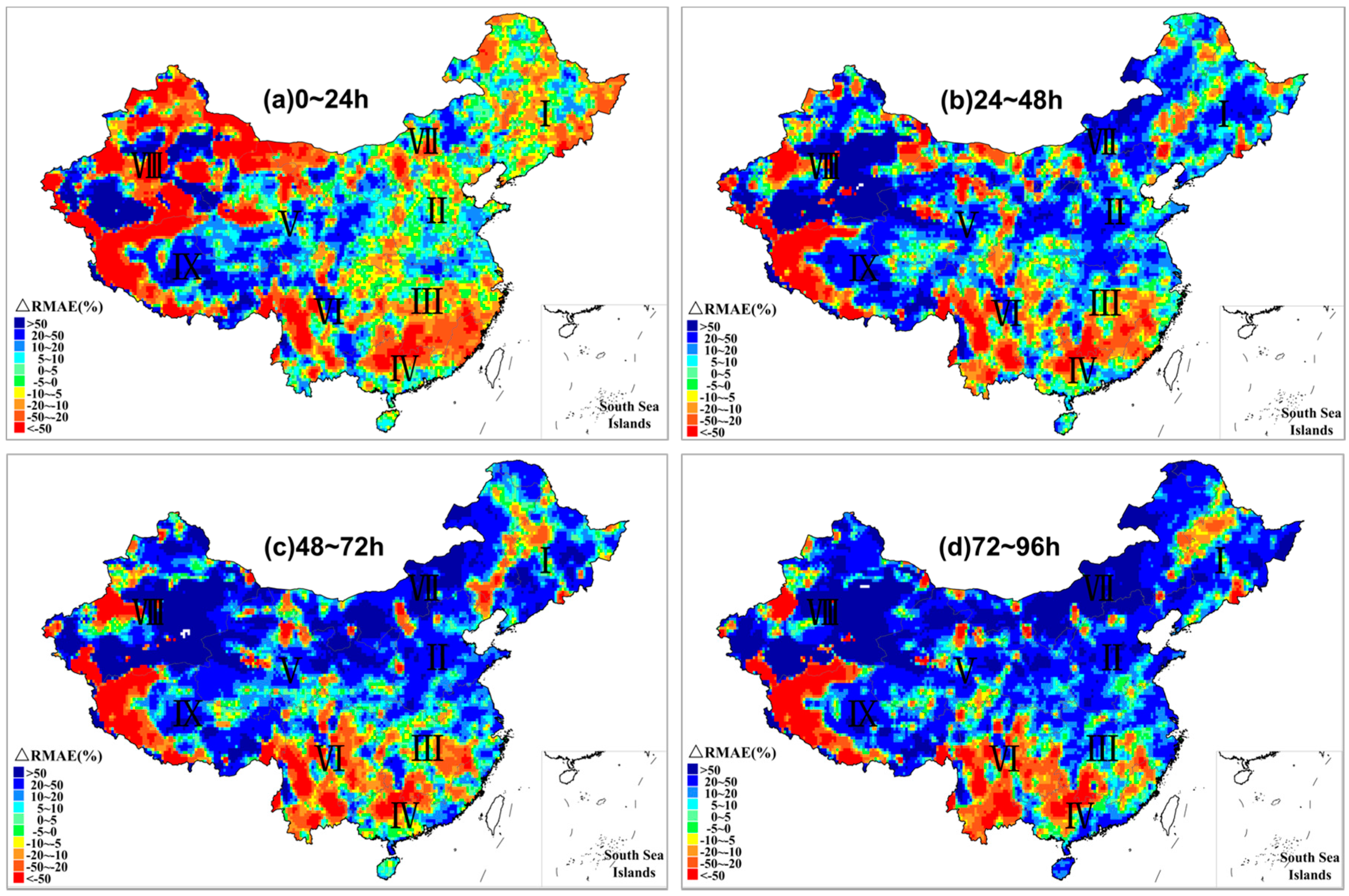
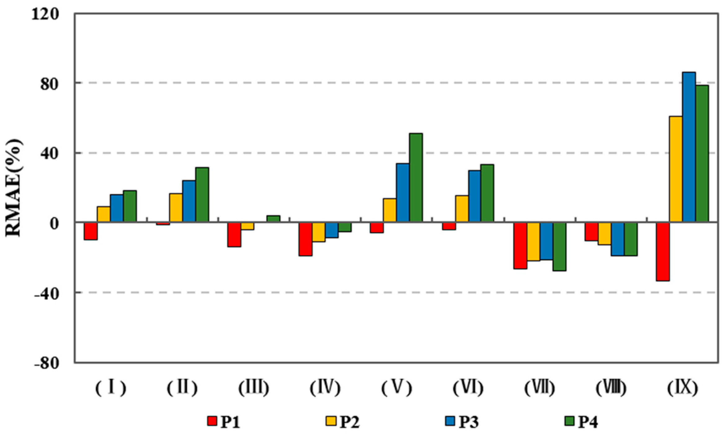
3.1.2. Spatial Distribution Characteristics

In this part, we calculated the temporal average of each grid around China of R and RMAE to directly understand the spatial characteristics of forecast skills with a lead time of 144 h. The characteristics of the forecast periods from 72–96 h and from 96–120 h are similar to those of 48–72 h and 96–120 h respectively, so only the results for the other four forecast periods are presented in this section.
We can see from Figure 3a that there is a significant positive correlation between corresponding observations and forecasts at different forecast periods and the R values decrease regionally with the extension of forecast period. In particular, the variations of R in the central and southern parts of Xinjiang (VIII), northern and central part of Tibet (IX) and the eastern part of Northwest (V) are relatively small (below 0.5). In other areas, the variation is more significant, where the R value is greater than 0.5, even up to 0.8 in some areas, for the forecast period 0–24 h and 24–48 h and less than 0.5 or even 0.2 when the lead time is longer than 72 h.
Comparing Figure 3b with Figure 3c, the R values between the flood season and the non-flood season in South (IV), East (III) and Southwest (VI) are similar. The values in Xinjiang (VIII), northern Tibet (IX), Inner Mongolia (VII) and northern part of Northeast (I) are from 0 to 0.2. The R in the junction among Xinjiang (VIII), Northwest (V) and Inner Mongolia (VII) is almost 0 in the non-flood season and the proportion for 120–144 h is the smallest. In different forecast periods, the correlation coefficient of flood season was higher in 24–48 h and 48–72 h than that in other periods and for the same forecast period, the values of flood and non-flood season were lower than that of annual average.
For the moderate rainfall forecast and above (Figure 3d), the R is much less than that in Figure 3a, which is below 0.4 around China. The variation in different forecast periods is relatively milder than Figure 3a–c. There are some high values of R in Xinjiang (VIII), Northwest(V), Tibet (IX) and Inner Mongolia(VII), while R in the southwestern part of Xinjiang (VIII), northern Tibet (IX), northern Northwest (V) and midwestern Inner Mongolia (VII) are still negative for all the forecast periods, with insignificant differences in area proportion, indicating a relative poor correlation between observations and forecasts in these sub-regions.
As shown in Figure 4, the spatial distribution for average RMAE around the year (Figure 4a) and that for the flood season (Figure 4b) are similar. In the 0–24 h forecast period, the RMAE values in Mideastern parts is below 100%. And RMAE in the flood season is slightly higher than that of the multi-year average. Meanwhile, the RMAE is about 130% when the lead time is longer than 72 h. For all the forecast periods, the RMAE values in Xinjiang (VIII) and Tibet (IX) are higher than 130%. In particular, RMAE is up to 250% in the south of Xinjiang (VIII), slightly increasing in area with the increase in lead time. And the area where the value is lower than 250% in flood season is smaller than the multi-year average.
With the extension of the forecast period, the area where the RMAE in the non-flood season (Figure 4c) reaches 250% extends northeastwards to Northeast (I), westwards to the central part of Southwest (VI), southeastwards to southeastern Northwest (V) from midsouthern part of Xinjiang (VIII), Tibet (IX), midwest of Northwest (V) and west part of Inner Mongolia (VII), gradually increasing.
In the Northeast (I), North (II), East (III) and South (IV) regions, the RMAE in the non-flood season is slightly lower than that in (a) and (b) when the lead time is shorter than 48 h. For most areas, the value is below 50% for the forecasts 0–24 h. When the lead time is longer than 48 h, the forecast skill in non-flood season is similar to the multi-year average and the flood season.
From Figure 4d, the RAME for moderate rainfall forecast and above is not greater than 100%, the maximum value area range increases with the extension of forecast period, still occurring in the junction of Xinjiang (VIII), Tibet (IX) and Northwest (V) and when the lead time is longer than 72 h, the RMAE in the other regions is higher than 60%. In the same forecast period, the RMAE for moderate rainfall and above is lower than that in multi-year average (a), the flood season (b) and the non-flood season (c). When the lead time is shorter than 48 h, the low value range appeared in the midsouthern parts of Northeast (I), central Inner Mongolia (VII), central Northwest (V) and midwestern regions of East (III).

3.2. Temporal Distribution of Forecast Skill

3.2.1. Monthly Variations

Figure 5 shows the monthly series for R, AI, MBE and RMAE around China. It can be seen that the monthly variation of each metric is similar for all different forecast periods.
From Figure 5a, it can be seen that the monthly R decreases with the extension of the forecast period and has no significant differences. The highest values are in May (lead time is shorter than 120 h) and June (the forecast period is 120–144 h) and the lowest ones are in January and December. Statistically, when the forecast period is 0–24 h and 24–48 h, the monthly R in May and June is above 0.46, the highest value reaches 0.59 and 0.55 respectively, while the values in January and December are 0.49/0.48 and 0.46/0.47. R in these two periods increase from January to May and then gradually decrease to September and then slightly increase until a sharp decrease in December.
When the lead time is longer than 48 h, the monthly R is less than 0.5, the highest in February and November while the lowest in summer. For these four forecast periods, R obviously increases from January to February and decreases from March to August and then again increases to November and then decreases significantly in December. The monthly variation of R indicates that the related degree between forecasts and observed precipitation of the GEM model in summer is slightly worse than that in other seasons.
It can be seen from Figure 5b that the monthly AI is less than 1 for different forecast periods, indicating that the GEM model can predict the precipitation at the lead time of 144 h to a certain degree. In all forecast periods, AI increases with the forecast period, which suggests that the random error of the model increases as well. In the same forecast period, the monthly differences are not significant. Comparatively speaking, the lowest value appears in May and the highest one is in winter. The index value in summer is a little lower than that in spring and fall, whose values are similar.
It can be seen from Figure 5c that as the lead time extends, the monthly MBE increases. Except for the negative MBE (−0.14 and −0.04) in July and August for the forecast period 0–24 h, the monthly values are not less than 0, indicating that the forecasts of GEM are slightly higher than the observations. For all the forecast periods, the MBE is the highest in April and lowest in July. And when the lead time is longer than 24 h, MBE in July is below 0. The monthly series of MBE is similar to that of R, lowest in summer, highest in spring and winter is a little higher than autumn.
Figure 5d shows that the RMAE is higher than 100% for all months except June and July. And the RMAE from June to September is less than 150%. For all the forecast periods, the values of RMAE increase as the lead time increases. When the lead time is shorter than 96 h, the monthly increase between two adjacent forecast periods is almost the same and the smallest increase is in the summer, about 10% to 15%, while the most obvious increase is in winter with 120%. When the lead time prolongs to 96 h, the RMAE in November obviously increases, the value of for 96–120 h and 120–144 h is 1355% and 1883% respectively. The monthly variation characteristics of RMAE are similar with that R and MBE.
To further understand the temporal predictive ability of the GEM model for different precipitation categories, the TS and BS values were used.
As shown in Figure 6, the change in monthly TS becomes more consistent for all forecast periods from moderate rainfall to the trace of rainfall. For the trace of rainfall and little rainfall forecast, the TS from June to August (summer) are higher than those in other months and the lowest are in January and December (winter). The values in spring and autumn are about the same. The TS of moderate rainfall forecast is the highest in May and the lowest also in January and December. The forecast skills are almost the same in spring, summer and winter, which are a little more desirable than that in winter. The monthly changes in heavy and extreme rainfall forecast are obvious. For heavy rainfall forecast, the forecast skill for different forecast periods are similar. In general, TS in summer and autumn are higher than that in winter and spring in the 0–24 h and 24–48 h. When the lead time is longer than 72 h, the monthly TS are almost the same, lower than 0.1. The monthly changes of TS of the extreme rainfall forecast do not have consistency. The value in summer for 0–24 h is around 0.1 while others are less than 0.1, which indicates that the GEM model has poor forecast ability for heavy and extreme rainfall.
Figure 7 illustrates the monthly variation of multi-year average of BS. The monthly variations of BS in the trace of rainfall and little rainfall forecast are consistent with each other. Statistically, BS in the trace of rainfall in summer is less than 2, indicating that the predicted area by GEM is below twice more than the measured area. Meanwhile, BS in winter is higher than 7, with an obvious vacancy forecast. The monthly BS values for moderate rainfall are all greater than 1, while that in May to September are below 2. The monthly variations differ in different forecast periods. For the forecast period 0–24 h, the monthly change is small from 1.1 to 2.5. For the lead time from 24–96 h, the monthly series are similar. The values in January are the highest and then slightly decrease in the following two months and after that gradually decrease from April to August then slowly increase until the next January. When the lead time is longer than 96 h, the monthly change process is similar to that of 24–96 h but there is a sharp increase from November to December. For heavy rainfall, BS from June to September are about 1, which indicates that the heavy rainfall forecast area of GEM in summer is almost identical with observations. When the lead time is longer than 24 h, BS in spring and winter are higher than 1, especially in February and March for 120–144 h, indicating GEM overestimates the heavy rainfall area in these two seasons when the lead time is longer than 24 h. For extreme rainfall forecasts, the monthly variations are more complicated. For 0–48 h forecasts, monthly BS are not greater than 1, except for April in 24–48 h forecast, suggesting that the GEM model underestimates the precipitation area. For other four forecast periods, BS in January to March are lower than 1 and that in April to June are around 1. BS for July to December are above 1, especially for the lead time longer than 48 h, BS in November and December are up to 5.

3.2.2. Forecast Skill in Flood and Non-Flood Season

Due to the uneven distribution of precipitation during a year in China, the precipitation in flood season is more abundant than that in non-flood season and the corresponding weather conditions are also different. Therefore, the numerical model forecast skills are different in these two periods. In the study, we divided the study period into flood season (from May to October) and non-flood season (November to April). The multi-year average TS and BS values in flood season and non-flood season are calculated respectively to compare the effect of GEM model in these two periods.
Figure 8 and Figure 9 show the multi-year average TS and BS for different forecast periods in the nine sub-regions of flood and non-flood season from 2009 to 2013. From Figure 8, it can be seen that the TS value in the flood season is higher than that in the non-flood season, i.e., the forecast skill of the GEM model in flood season is better than the non-flood season. But there are also differences in the prediction skill in different sub-regions in these two periods. In general, the TS differences of the trace of rainfall and little rainfall are greater than that of the other three precipitation categories. For the trace of rainfall and little rainfall forecast, the difference of forecast skill is the most significant in Northwest (V), Tibet (IX) and Southwest (VI). On average, the differences between the flood and non-flood season in the three regions are greater than 0.3 for the trace of rainfall. In Northwest (V) and Tibet (IX), the differences of little rainfall forecast are above 0.2, while in Southwest (VI), the difference is about 0.12. In Northeast (I) and Inner Mongolia (VII), the differences for trace of rainfall are both about 0.25, while the differences of the little rainfall are 0.07–0.13 and 0.09–0.16, respectively. The difference in South (IV) for trace of rainfall is about 0.15 and almost the same for little rainfall. In East (III), the prediction skill is similar for trace of rainfall and little rainfall forecast. For moderate and above forecasts, the forecast skill between in all regions is similar between these two periods and there is little forecast ability for heavy rainfall.
From Figure 9, it can be seen that the BS in flood season is lower than that in non-flood season and the difference for these two periods for the trace of rainfall is higher than other precipitation categories. In particular, for trace of rainfall and little rainfall forecast, the difference in Northwest (V) is the highest. Next comes the difference in the Inner Mongolia (VII) and Tibet (IX), followed by that in the Northeast (I) and Southwest (VI), about 20. In North (II), South (IV) and Xinjiang (VIII), the difference is about 10, while the difference in Xinjiang (VIII) is obviously higher than that of the other two sub-regions. The differences in East (III) for all precipitation categories are the least among the nine regions, ranging from 3.6 to 10.6. For heavy rainfall forecast in Xinjiang (VIII) as well as the extreme rainfall forecast in all sub-regions except for the North (II), East (III) and South (IV), the BS value is less than 1, suggesting that missing report also occurs. Meanwhile, the BS values in Inner Mongolia (VII), Northwest (V), Southwest (VI) and Xinjiang (VIII) for non-flood season are about 0, suggesting that the GEM model can hardly predict the extreme rainfall in these regions all the year around.

4. Discussion

4.1. Performance Comparison with GFS

The medium-range model, GEM used in the study, has a higher resolution than many other models and the model developers have been working on the improvement of the forecast skill. Nevertheless, previous studies have shown that high resolution does not always mean more skillful forecasts. The resolution in the study is much higher than that in [24]. They compared the forecast skill of the new GEM with the resolution of 33 km with that of the old GEM model with the resolution of 100 km. The results show that GEM with higher resolution can better agree with the observations over North America. They analyzed the ETS and BS of the GEM model with the lead time of 120 h for different precipitation categories, using the 0–24 h, 48–72 h and 96–120 h accumulative precipitation.
To further recognize whether the GEM model performs better in China at a higher resolution, we also compared the skills using ETS and BS over China and North America. Figure 10 shows the ETS and BS over China for different precipitation categories. The comparison of these two scores demonstrates that the ETS over China is similar to that over North America, while the BS over China is much higher than that in North America. Therefore, the degrees of coincidence between forecasts and observations are similar in China and North America but the vacancy rate of the model in China is much higher than the model of 33 km in North America. It is perhaps caused by the parameterization of GEM, which is necessary to propose improvement in China.
In the study, the comparison between the forecast skill of GEM and GFS, with the resolution of 1°, was also conducted for the lead time of 96 h in 2011 to further investigate the GEM forecast skill. Figure 11 shows the TS and BS for GEM and GFS. In general, the forecast skills for the two models are almost similar as well as some differences for TS and the BS values for these two models are different. For TS, we can see that for the forecast period 0–24 h, the GEM model is a little better than GFS. For the other forecast periods, the GEM model is slightly more skillful in moderate rainfall forecast and above, while in trace of rainfall and little rainfall forecast, the GFS model is a little better. For the BS score, GFS is much better than GEM. There are many vacancy forecasts for both models but the forecasts area of GEM is much larger than that of GFS. Therefore, compared to the GFS model, the GEM model is of similar consistency with the observations while the forecast area is dramatically larger.
The investigation into the spatial distribution differences of R and RAME, shown in Figure 12 and Figure 13, between GEM and GFS were also conducted. The difference is defined as the multi-year average R/RMAE value of GEM minus that of GFS of each grid. From Figure 12 we can see that these two models have similar forecast skill over most parts of China for all the forecast periods. The area where the R of GEM is greater than that of GFS decreases with the increase of lead time. The obvious differences occur around Inner Mongolia (VII), Northwest (V), mid-Xinjiang (VIII) and Northern Tibet (IX). But for the RMAE (Figure 13), the values of GEM are much higher than that of GFS and with the increase in lead time, the area of higher value of GEM than GFS increases dramatically. The lowest value for the difference is in the southeastern Tibet (IX) and the junction between Southwest (VI), South (IV) and East (III). Therefore, for the forecasts of 0–24 h, the GEM model has a more desirable forecast skill than the GFS model but with the extension of lead time, the GEM’s skill decreases.
Figure 14 shows the RMAE differences between GEM and GFS in nine sub-regions, to directly obtain the spatial average difference. We can see that in 8 sub-regions (except Tibet (IX)), the RMAE differences range from −40% and 40%, especially in East (III), the difference values are −13.6%, −4.1%, 0 and 4.2% for four forecast periods, respectively; while in Tibet (IX), RMAE of GEM is up to 80% larger than that of GFS in the forecast period 48–72 h. Meanwhile, for forecast period 0–24 h, the RMAE of GEM is smaller than GFS. In South (IV), Inner Mongolia (VII) and Xinjiang (VIII), GEM performs better in the lead time of 0–96 h and in East (III), GEM is more skillful except in 72–96 h. We also conducted the regionally differences of R in nine sub-regions (results are not shown here), almost all of the differences are 0, which indicates that both of the forecasts of these two models correspond well with the observations regionally.

4.2. Overview

We can see from the results that the GEM model performs better in East and Central China, especially for the flood season in South (IV), East (III) and North (I). However, in Xinjiang (VIII), Inner Mongolia (VII) and Tibet (IX), the forecast ability is a little poor. On the one hand, during flood season, more precipitation caused by monsoon occurs compared with non-flood season, the precipitation distribution is maybe more in line with the parameterization of the model. So as to the comparison between south coast and the inland area. On the other hand, the greater precipitation variability [51] in Xinjiang (VIII), Inner Mongolia (VII) and Tibet (IX) may cause that the dynamic model and parameterization of GEM cannot always fully reflect the realistic atmospheric motions. Meanwhile, one of the reasons for the model performs better in East, South and Central China is topography. Ren et al. [52] pointed out that the complexity of precipitation distribution is affected by topography to some degree and it is not easy to reflect the high-latitude area atmospheric motions. Another reason is that the gridded observations we used in the study perform better in East, South and Central China [28], for there are more stations in these regions, providing a more convincing observation, while in other regions, the observations are not insufficient. And the results are coincident with previous research using other NWPs both at home and abroad [15,16,17,18,19,39,40,41,42,50]. For different categories, the forecast skills for heavy and storm precipitation are worse than that of trace of rainfall or little precipitation. The reason is that occurrence of heavy and storm rainfall is related to mesoscale weather system and the mechanism and parameterization cannot reflect the real distribution information effectively. The results are also coincident with that in Canada [24]. And the relatively poor forecast performance for heavy and storm rainfall is a common drawback in NWP models [42].
Mcbride and Ebert [53] pointed out that the precipitation threshold used affected the verification of forecast skill. Though the precipitation categories used in the study are with lower and upper threshold and the forecast is more detailed and strict compared with the previous studies, the forecast skill of the GEM model is similar to or better than that of other models [18,54], which fully explains the application of the GEM model in China. However, the GEM model with a higher resolution than GFS does not present a much better performance instead, which motivates an in-depth comparison between the mechanisms of GEM and GFS, to further understand the reasons and then propose the method to improve the forecast skill of GEM with high-resolution. Meanwhile, in the study, we only focused on the forecast skill of the GEM model, paying no attention to the investigation into the inner mechanism. The dynamic model and parameterization of GEM, affected by precipitation mechanism, topography as well as precipitation scale, are key factors in model performance. Therefore, more improvement needs to be proposed in the future study, such as the characteristics of performance variability, the reasons for the difference of the performance variability regionally, the relationship between precipitation variability and performance variability, etc.
The results we obtained in the study is a solid foundation to adopt the GEM model in China. For example, in terms of hydrological prediction, we can use the forecasts, coupled with hydrological models to predict extreme hydrological events, such as floods and droughts. Wu has conducted a similar research and it shown that the flood forecasts is performed both in meteorological and discharge prediction [22]. Besides, it is also a tool to use GEM in soil moisture detection and prediction to help make a more convincing strategy in ahead of time. However, we also need to pay more attention to the improvement of forecasts for the forecast skill does not always enhance with the increasing of resolution. And how about the prediction performance with the increasing resolution as well in the next coming steps.

5. Conclusions

In recent years, with the development of NWP, the precipitation forecast skill also gradually increases, which is beneficial to prolong the lead time of quantitative precipitation forecasts. The study is to evaluate the forecast skill of the medium-range GEM model with high resolution in China, with the lead time of 144 h. Based on the 24 h accumulative observations, the study explored the temporal and spatial skill of the model, as well as for the flood and non-flood season. The results show that the forecast skill divers obviously temporally and spatially.
Generally, with the increase in precipitation categories and lead time, the forecast ability of the GEM model declines dramatically. The GEM model often provides a larger precipitation area than observations, especially estimating whether precipitation occurs or there is little rainfall. And in spatial, the forecast skill decreases northwestwards from Southeast China. In detail, for the trace of rainfall and little rainfall, the forecast skill in Southwest and East varies more obviously with lead time than other sub-regions, especially for Xinjiang. For moderate rainfall and above, the forecast skill is poor to some degree, especially in western China, such as Xinjiang and Tibet. For different forecast periods, the model is relatively more skillful for 0–96 h lead time forecast in Northeast, North, East and South and for 96–144 lead time, the skill is not ideally enough. Meanwhile, the forecast skill in flood season (summer and autumn) is better than that in non-flood season (spring and winter). However, the performance of these two periods in South, East and Southwest are similar. The monthly variance tendency for each forecast period are similar and the variance of performance difference is of significance with rainfall area bias. The results here indicate it is appropriate to use the GEM model in China to some degree, both in weather forecast and meteorological and hydrological prediction in the future.

Acknowledgments

This work is supported by the National Key Research and Development Project (2017YFC1502403), the National Science Foundation of China (Grant Nos. 51579065, 51779071), the Fundamental Research Funds for the Central Universities (Grant No. 2017B10514), Central Public Welfare Operations for Basic Scientific Research of Research Institute (Grant No. HKY-JBYW-2017-12) and Water Science and Technology Project of Jiangsu Province (2017007).

Author Contributions

H.X. and Z.W. conceived and designed the experiments; H.X. performed the experiments; H.X. and H.H. analyzed the data; Z.W. and L.L. contributed reagents/materials/analysis tools; H.X. and L.L. wrote the paper. All authors read and approved the final manuscript.

Conflicts of Interest

The authors declare that they have no conflict of interests. The founding sponsors had no role in the design of the study; in the collection, analyses, or interpretation of data; in the writing of the manuscript and in the decision to publish the results.

References

  1. Krzysztofowicz, R. The case for probabilistic forecasting in hydrology. J. Hydrol. 2001, 249, 2–9. [Google Scholar] [CrossRef]
  2. Biondi, D.; Luca, D.L.D. Performance assessment of a Bayesian Forecasting System (BFS) for real-time flood forecasting. J. Hydrol. 2013, 479, 51–63. [Google Scholar] [CrossRef]
  3. Liu, D.; Li, X.; Guo, S.; Dan, R.; Chen, H. Using a Bayesian Probabilistic Forecasting Model to Analyze the Uncertainty in Real-Time Dynamic Control of the Flood Limiting Water Level for Reservoir Operation. J. Hydrol. Eng. 2015, 20, 4014036. [Google Scholar] [CrossRef] [Green Version]
  4. Ciupak, M.; Ozga-Zielinski, B.; Adamowski, J.; Quilty, J.; Khalil, B. The application of Dynamic Linear Bayesian Models in hydrological forecasting: Varying Coefficient Regression and Discount Weighted Regression. J. Hydrol. 2015, 530, 762–784. [Google Scholar] [CrossRef]
  5. Reggiani, P.; Weerts, A.H. Probabilistic Quantitative Precipitation Forecast for Flood Prediction: An Application. J. Hydrometeorol. 2008, 9, 76–95. [Google Scholar] [CrossRef]
  6. Wilks, D.S. Statistical Methods in the Atmospheric Sciences; Elsevier: Amsterdam, The Netherlands, 2005; pp. 183–197. ISBN 978-0-12-751966-1. [Google Scholar]
  7. French, M.N.; Bras, R.L.; Krajewski, W.F. A Monte Carlo study of rainfall forecasting with a stochastic model. Stoch. Hydrol. Hydraul. 1992, 6, 27–45. [Google Scholar] [CrossRef]
  8. Versace, P.; Sirangelo, B.; Luca, D.L.D. A space-time generator for rainfall nowcasting: the PRAISEST model. Hydrol. Earth Syst. Sci. Discuss. 2009, 13, 441–452. [Google Scholar] [CrossRef]
  9. Metta, S.; Hardenberg, J.V.; Ferraris, L.; Rebora, N.; Provenzale, A. Precipitation nowcasting by a spectral-based nonlinear stochastic model. J. Hydrometeorol. 2010, 10, 1285–1297. [Google Scholar] [CrossRef]
  10. Nicholls, N.; Dyer, T.G.J. Comment on the paper ‘On the application of some stochastic models to precipitation forecasting’ by T. G. J. Dyer. Q. J. R. Meteorol. Soc. 2010, 103, 177–189. [Google Scholar] [CrossRef]
  11. Laio, F.; Tamea, S. Verification tools for probabilistic forecasts of continuous hydrological variables. Hydrol. Earth Syst. Sci. 2007, 11, 1267–1277. [Google Scholar] [CrossRef]
  12. Kumar, P.; Kishtawal, C.M.; Pal, P.K. Skill of regional and global model forecast over Indian region. Theor. Appl. Climatol. 2016, 123, 629–636. [Google Scholar] [CrossRef]
  13. Mass, C.F.; Ovens, D.; Westrick, K.; Colle, B.A. Does Increasing Horizontal Resolution Produce More Skillful Forecasts? Bull. Am. Meteorol. Soc. 2002, 83, 407–430. [Google Scholar] [CrossRef]
  14. Roberts, N. Assessing the spatial and temporal variation in the skill of precipitation forecasts from an NWP model. Meteorol. Appl. 2008, 15, 163–169. [Google Scholar] [CrossRef]
  15. Chakraborty, A. The Skill of ECMWF Medium-Range Forecasts during the Year of Tropical Convection 2008. Mon. Weather Rev. 2010, 138, 3787–3805. [Google Scholar] [CrossRef]
  16. Durai, V.R.; Bhowmik, S.K.R. Prediction of Indian summer monsoon in short to medium range time scale with high resolution global forecast system (GFS) T574 and T382. Clim. Dyn. 2013, 42, 339. [Google Scholar] [CrossRef]
  17. Pan, L.J.; Xue, C.F.; Zhang, H.F.; Wang, J.P.; Yao, J. Comparison of Three Verification Methods for High-Resolution Grid Precipitation Forecast. Clim. Environ. Res. 2017. (In Chinese) [Google Scholar]
  18. Meng, Y.J.; Wu, H.B.; Wang, L.; Zhang, P.P. Evaluation of Quantitative Precipitation Estimation of Numerical Weather Prediction Models in Wuhan Region during Main Flood Season of 2007. Torrential Rain Disasters 2008, 12, 73–77. (In Chinese) [Google Scholar] [CrossRef]
  19. Novak, D.R.; Bailey, C.; Brill, K.F.; Burke, P.; Hogsett, W.A.; Rausch, R.; Schichtel, M. Precipitation and Temperature Forecast Performance at the Weather Prediction Center. Weather Forecast. 2014, 29, 489–504. [Google Scholar] [CrossRef]
  20. Liu, Y.; Duan, Q.Y.; Zhao, L.N.; Ye, A.Z.; Tao, Y.M.; Miao, C.Y.; Mu, X.; Schaake, J.C. Evaluating the predictive skill of post-processed NCEP GFS ensemble precipitation forecasts in China’s Huai river basin. Hydrol. Process. 2013, 27, 57–74. [Google Scholar] [CrossRef]
  21. Cote, J. The operational CMC-MRB Global Environmental Multiscale (GEM) Model. Part I. Design consideration and formulation. Mon. Weather Rev. 1998, 126, 1373–1395. [Google Scholar] [CrossRef]
  22. Wu, J.; Lu, G.H.; Wu, Z.Y. Flood forecasts based on multi-model ensemble precipitation forecasting using a coupled atmospheric-hydrological modeling system. Nat. Hazards 2014, 74, 325–340. [Google Scholar] [CrossRef]
  23. Markovic, M.; Lin, H.; Winger, K. Simulating Global and North American Climate Using the Global Environmental Multiscale Model with a Variable-Resolution Modeling Approach. Mon. Weather Rev. 2010, 138, 3967–3987. [Google Scholar] [CrossRef]
  24. Bélair, S.; Roch, M.; Leduc, A.M.; Vaillancourt, P.A.; Laroche, S.; Mailhot, J. Medium-Range Quantitative Precipitation Forecasts from Canada’s New 33-km Deterministic Global Operational System. Weather Forecast. 2009, 24, 690. [Google Scholar] [CrossRef]
  25. Zadra, A.; Caya, D.; Côté, J.; Dugas, B.; Jones, C.; Laprise, R.; Winger, K.; Caron, L.P. The next Canadian Regional Climate Model. Phys. Can. 2008, 64, 75–83. [Google Scholar]
  26. Erfani, A.; Méthot, A.; Goodson, R.; Bélair, S.; Yeh, K.S.; Côté, J.; Moffet, R. Synoptic and mesoscale study of a severe convective outbreak with the nonhydrostatic Global Environmental Multiscale (GEM) model. Meteorol. Atmos. Phys. 2003, 82, 31–53. [Google Scholar] [CrossRef]
  27. China Meteorological Scientific Data Sharing Website. Available online: http://data.cma.cn/ (accessed on 6 June 2014).
  28. Shen, Y.; Xiong, A.Y. Validation and comparison of a new gauge-based precipitation analysis over mainland China. Int. J. Climatol. 2016, 36, 252–265. [Google Scholar] [CrossRef]
  29. GDPS data in GRIB2 format: 25 km. Available online: https://weather.gc.ca/grib/grib2_glb_25km_e.html (accessed on 31 December 2013).
  30. Zhu, Z.W.; Li, T. Extended-range forecasting of Chinese summer surface air temperature and heat waves. Clim. Dyn. 2017, 1–15. [Google Scholar] [CrossRef]
  31. Zhu, Z.W.; Li, T.; Bai, L.; Gao, J.Y. Extended-range forecast for the temporal distribution of clustering tropical cyclogenesis over the western North Pacific. Theor. Appl. Climatol. 2016, 130, 1–13. [Google Scholar] [CrossRef]
  32. Zhu, Z.W.; Li, T. Statistical extended-range forecast of winter surface air temperature and extremely cold days over China. Q. J. R. Meteorol. Soc. 2017, 143, 1528–1538. [Google Scholar] [CrossRef]
  33. Zhu, Z.W.; Li, T.; Hsu, P.C.; He, J.H. A spatial-temporal projection model for extended-range forecast in the tropics. Clim. Dyn. 2015, 45, 1085–1098. [Google Scholar] [CrossRef]
  34. Zhu, Z.W.; Li, T. The statistical extended-range (10–30-day) forecast of summer rainfall anomalies over the entire China. Clim. Dyn. 2016, 48, 1–16. [Google Scholar] [CrossRef]
  35. Zhu, Z.W.; Chen, S.J.; Yuan, K.; Chen, Y.N.; Gao, S.; Hua, Z.F. Empirical Subseasonal Prediction of Summer Rainfall Anomalies over the Middle and Lower Reaches of the Yangtze River Basin Based on Atmospheric Intraseasonal Oscillation. Atmosphere 2017, 8, 185. [Google Scholar] [CrossRef]
  36. Office of State Flood Control and Drought Relief Headquarters and Nanjing Institute of Hydrology and Water Resources. China Flood and Drought Disaster; China Water Power Press: Beijing, China, 1997; p. 569. ISBN 7-80124-422-2. (In Chinese) [Google Scholar]
  37. Wu, Z.Y.; Lu, G.H.; Wen, L.; Lin, C.A. Reconstructing and analyzing China’s fifty-nine year (1951–2009) drought history using hydrological model simulation. Hydrol. Earth Syst. Sci. 2011, 8, 2881–2894. [Google Scholar] [CrossRef] [Green Version]
  38. Zhang, Z.M.; Zhang, C.C.; Hou, H.Y.; Wang, Y.Z. Application of Grade of Precipitation (GB/T 28592-2012). Modern Agric. Sci. Technol. 2016, 19, 223. (In Chinese) [Google Scholar]
  39. Lian, L.; Lin, K.P.; Huang, H.H. Comparison on Precipitation Forecast Effects of Several Numerical Prediction Models in Guangxi. J. Meteorol. Res. Appl. 2012. (In Chinese) [Google Scholar] [CrossRef]
  40. Zhao, N.K.; Wan, S.Y.; Qi, M.H. Precipitation verification of three models during rainy season in Yunnan province. J. Meteorol. Environ. 2015, 5, 39–44. (In Chinese) [Google Scholar]
  41. Gao, S.Y.; Sun, L.Q. Verification of JMH′s NWP on Rainfall Forecast in Dandong, Liaoning Province. Meteorological 2006, 32, 79–83. (In Chinese) [Google Scholar] [CrossRef]
  42. Dong, Y.; Liu, S.D.; Wang, D.H.; Zhao, Y.F. Assessment on Forecasting Skills of GFS Model for Two Persistent Rainfalls over Southern China. Meteorol. Mon. 2015. (In Chinese) [Google Scholar] [CrossRef]
  43. Colle, B.A.; Mass, C.F.; Westrick, K.J. MM5 Precipitation Verification over the Pacific Northwest during the 1997 99 Cool Seasons. Weather Forecast. 2000, 15, 730–744. [Google Scholar] [CrossRef]
  44. Eerola, K. Twenty-One Years of Verification from the HIRLAM NWP System. Weather Forecast. 2012, 28, 270–285. [Google Scholar] [CrossRef]
  45. White, B.G.; Paegle, J.; Steenburgh, W.J.; Horel, J.D.; Swanson, R.T.; Cook, L.K.; Onton, D.J.; Miles, J.G. Short-Term Forecast Validation of Six Models. Weather Forecast. 1998, 14, 84–108. [Google Scholar] [CrossRef]
  46. Koh, T.Y.; Ng, J.S. Improved diagnostics for NWP verification in the tropics. J. Geophys. Res. Atmos. 2009, 114, 1192. [Google Scholar] [CrossRef]
  47. Wang, Y.; Yan, Z.H. Effect of Different Verification Schemes on Precipitation Verification and Assessment Conclusion. Meteorol. Mon. 2007, 33, 53–61. (In Chinese) [Google Scholar] [CrossRef]
  48. Hayashi, S.; Aranami, K.; Saito, K. Statistical Verification of Short Term NWP by NHM and WRF-ARW with 20 km Horizontal Resolution around Japan and Southeast Asia. Sci. Online Lett. Atmos. Sola 2008, 4, 133–136. [Google Scholar] [CrossRef]
  49. Chen, C.J.; Jun, L.I.; Wang, M.H. Verification of precipitation forecast using an operational numerical model during flooding season of 2013 in the middle area of China. J. Meteorol. Environ. 2015, 2, 1–8. (In Chinese) [Google Scholar]
  50. Olson, D.A.; Junker, N.W.; Korty, B. Evaluation of 33 Years of Quantitative Precipitation Forecasting at the NMC. Weather Forecast. 1995, 10, 498–511. [Google Scholar] [CrossRef]
  51. Zhou, T.J.; Qian, Y.F. An experimental study on the effects of topography on numerical prediction. Sci. Atmos. Sin. 1996. (In Chinese) [Google Scholar] [CrossRef]
  52. Ren, G.Y.; Zhan, Y.J.; Ren, Y.Y.; Chen, Y.; Wang, T.; Liu, Y.X.; Sun, X.B. Spatial and temporal patterns of precipitation variability over mainland China: I: Climatology. Adv. Water Sci. 2015, 26, 299–310. (In Chinese) [Google Scholar] [CrossRef]
  53. Mcbride, J.L.; Ebert, E.E. Verification of Quantitative Precipitation Forecasts from Operational Numerical Weather Prediction Models over Australia. Weather Forecast. 1999, 15, 103–121. [Google Scholar] [CrossRef]
  54. Li, J.; Wang, M.H.; Gong, Y.; Li, C.; Li, W.J. Precipitation Verifications to an Ensemble Prediction System Based on AREM. Torrential Rain Disasters 2010. (In Chinese) [Google Scholar] [CrossRef]
Figure 1. The nine sub-regions of mainland China used in this study and average annual precipitation based on gridded observations at the resolution of 0.25° from 2009 to 2013.
Atmosphere 09 00104 g001
Figure 2. The average (a) TS (threat score) and (b) BS (bias score) value of nine sub-regions over China for different forecast periods and precipitation categories from 2009 to 2013 of GEM (Global Environmental Multi-scale Model). The (I) to (IX) here represent Northeast, North, East, South, Northwest, Southwest, Inner Mongolia, Xinjiang and Tibet respectively and the P1 to P6 here represent the 6 forecast periods from 0–24 to 120–144 h.
Atmosphere 09 00104 g002
Figure 3. The spatial distribution of R (correlation coefficient) between observations and the GEM forecasts for different forecast periods of the multi-year average for (a) all the precipitation, (b) the precipitation in flood season, (c) the precipitation in the non-flood season and (d) the moderate rainfall and above. P1, P2, P3 and P6 here represent the forecast periods of 0–24, 24–48, 48–72 and 120–144 h. The color of white represents negative correlation between observations and forecasts.
Atmosphere 09 00104 g003
Figure 4. The spatial distribution of RMAE (relative mean absolute error) between observations and the GEM forecasts for different forecast periods of the multi-year average for (a) all the precipitation, (b) the precipitation in flood season, (c) the precipitation in non-flood season and (d) the moderate rainfall and above. P1, P2, P3 and P6 here represent the forecast periods of 0–24, 24–48, 48–72 and 120–144 h.
Atmosphere 09 00104 g004
Figure 5. The monthly average for (a) R, (b) AI (alpha index), (c) MBE (mean bias error) and (d) RMAE between observations and the GEM forecasts for different forecast periods from 2009 to 2013 over China. P1 to P6 here represent the 6 forecast periods from 0–24 to 120–144 h.
Atmosphere 09 00104 g005
Figure 6. The monthly average TS for different periods and precipitation categories (ae respect: trace of, little, moderate, heavy and extreme rainfall) over China of GEM from 2009 to 2013. P1 to P6 here represent the 6 forecast periods from 0–24 to 120–144 h.
Atmosphere 09 00104 g006
Figure 7. The monthly average BS for different periods and precipitation categories (ae respect: trace of, little, moderate, heavy and extreme rainfall) over China of GEM from 2009 to 2013. P1 to P6 here represent the 6 forecast periods from 0–24 to 120–144 h.
Atmosphere 09 00104 g007
Figure 8. The average TS value of nine sub-regions over China in (a) flood and (b) non-flood season for different forecast periods and precipitation categories from 2009 to 2013 of GEM forecasts. The (I) to (IX) here represent Northeast, North, East, South, Northwest, Southwest, Inner Mongolia, Xinjiang and Tibet respectively and the P1 to P6 here represent the 6 forecast periods from 0–24 to 120–144 h.
Atmosphere 09 00104 g008
Figure 9. The average BS value of nine sub-regions over China in (a) flood and (b) non-flood season for different forecast periods and precipitation categories from 2009 to 2013 of GEM forecasts. The (I) to (IX) here represent Northeast, North, East, South, Northwest, Southwest, Inner Mongolia, Xinjiang and Tibet respectively and the P1 to P6 here represent the 6 forecast periods from 0–24 to 120–144 h.
Atmosphere 09 00104 g009
Figure 10. The results of (a) ETS (equitable threat score) and (b) BS over China of the different precipitation categories of GEM. P1 to P6 here represent the 6 forecast periods from 0–24 to 120–144 h.
Atmosphere 09 00104 g010
Figure 11. The comparison of (a) TS and (b) BS of GEM and GFS (Global Forecast System) for the lead time of 0–96 h. P1 to P4 here represent the 4 forecast periods from 0–24 to 72–96 h.
Atmosphere 09 00104 g011
Figure 12. The multi-year average spatial distribution of differences of R between GEM and GFS forecasts for different forecast period for the lead time of 96 h in 2011 (ad here represent the 4 forecast periods from 0–24 to 72–96 h).
Atmosphere 09 00104 g012
Figure 13. The multi-year average spatial distribution of differences of RMAE between GEM and GFS forecasts for different forecast period for the lead time of 96 h in 2011 (ad here represent the 4 forecast periods from 0–24 to 72–96 h).
Atmosphere 09 00104 g013
Figure 14. The regional difference of RMAE in nine sub-regions between GEM and GFS. The (I) to (IX) here represent Northeast, North, East, South, Northwest, Southwest, Inner Mongolia, Xinjiang and Tibet respectively and the P1 to P4 here represent the 4 forecast periods from 0–24 to 72–96 h.
Atmosphere 09 00104 g014
Table 1. The contingency table.
Observation
YesNo
ForecastYesNANB
NoNCND

