1. Introduction
The increase in the population density of many modern cities is limited by technical issues related to the construction of a healthy and effective living environment. In the short term, the citizens of such densely populated urban areas benefit from the scientific results of air quality research in the form of improved health conditions. Technological improvements may also allow for further increases in population density, therefore long-term benefits might be expected from the urbanization itself (e.g., by creating more job opportunities for individuals, faster development for local enterprises, and a more competitive economy at the national level).
Urban air quality displays large fluctuations in both space and time; therefore, the mitigation of extremely high local pollution conditions is of particular importance. The street canyon as a minimal model of a city is studied extensively from the perspective of flow structures and transport phenomena. The character of the flow is principally determined by the H/W ratio of the building height and street width [
1,
2]. The literature on street canyons was comprehensively reviewed by Vardoulakis et al. [
3] and Ahmad et al. [
4].
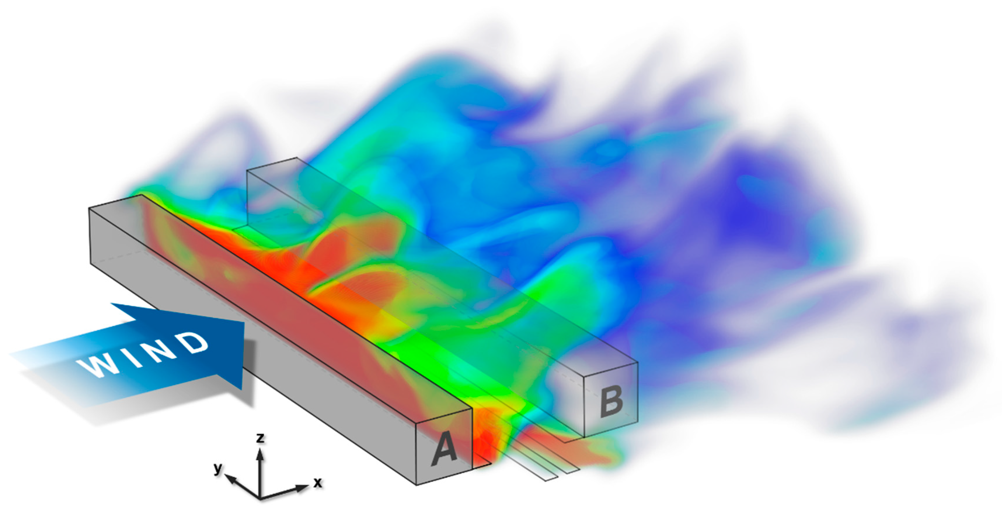
As can be seen later, the flow generated by the roof-level turbulent stresses can be characterized by one large vortex occupying almost the entire cross-section of the street canyon. The canyon vortex conveys airborne pollutants towards the leeward wall at a pedestrian level. At the same time, fresh air is transported to the sidewalk by the descending flow near the windward wall, causing a local concentration decrease. As can be seen from
Figure 1, there is a substantial concentration difference between the leeward and windward sides; the leeward side is critical regarding the pedestrian exposure to traffic induced pollution.
In practice, street-level air pollution can be mitigated by restricting emissions or by controlling the transmission process via geometrical changes. Buildings and other flow obstructions, such as urban vegetation, can be considered in the latter case. So far, most studies emphasizing the positive impact of urban vegetation are focused on the enhanced settling and filtering effects [
5,
6,
7], although only minor improvements of around 1% relative to the average street level concentration can be achieved in this way, because the hydraulic resistance of the vegetation limits the air flux through the volume occupied by the plants. Numerous other studies [
8,
9,
10,
11,
12,
13,
14] confirm that trees planted in the usual patterns decelerate the flow, thereby increasing the pollutant concentrations in critical locations, and this negative effect is at least one order of magnitude stronger than the gain from enhanced settling and filtering. The ambiguous impact of urban vegetation on air quality is comprehensively reviewed by Litschke and Kuttler [
15], and Janhaell [
16].
Based on a large eddy simulation (LES) model, McNabola et al. [
17] showed that low boundary walls may be used effectively for improving air quality at the street level. Even a relatively low wall in the middle of the street substantially modifies the flow; the canyon vortex splits into two counter-rotating vortices, and consequently, the street level flow is directed towards the middle of the street on both sides, thus decreasing the concentration at the leeward sidewalk. The favorable effect can also be observed if two low boundary walls are placed between the traffic lanes and sidewalks on the opposite sides of the street. Using a similar LES modelling method, Gallagher et al. [
18] showed that in asymmetric street canyons, the favorable effect of low boundary walls might be decreased or even reversed, therefore, a deeper investigation of the parametric dependencies is necessary.
Gromke et al. [
19] proved the favorable effect of central boundary walls with wind tunnel experiments on a finite-length street canyon model, and also pointed out that the improvement in air quality can also be realized by using hedgerows of limited permeability instead of boundary walls. The unfavorable effects of the permeability and discontinuity of the hedgerows were also investigated in a realistic parameter range.
Most microscale (building level) numerical dispersion models utilize the Reynolds averaged turbulence modelling approach, in which only the average field properties are computed, and the enhanced mixing—caused by unresolved unsteady flow structures—is modelled depending on the average flow properties. The computational cost can be substantially reduced with the help of the Reynolds averaged models, as the time dependency can be eliminated, and meaningful results can be obtained on relatively coarse meshes.
The Reynolds averaged approach has a number of shortcomings in urban air quality investigations [
20] (e.g., the lateral diffusion is underestimated), because such models cannot capture the effect of large-scale unsteady flow structures in the wake of buildings. Dispersion models are affected by turbulence modelling uncertainties in two ways. Firstly, by impacting the advection of pollutants through the inaccuracies of the velocity field, and secondly, by directly affecting the diffusive transport, therefore the concentration field is predicted with much greater uncertainty than the velocity field. Another shortcoming is that Reynolds averaged models do not provide sufficient information about concentration fluctuations, which limits the model’s applicability for assessing the health impact of toxic substances.
Globally unstable flows, attributed to the urban atmosphere, are usually more accurately predicted by scale-resolving turbulence models such as large eddy simulation (LES), detached eddy simulation (DES), or scale adaptive simulation (SAS) than by Reynolds averaged models. Best practice guidelines for scale resolving models are provided by Menter [
21]. The ability to resolve the three-dimensional unsteady flow structures stemming from flow instabilities is a common feature of these models. In LES models, the effect of small-scale unresolved turbulence is taken into account by using algebraic sub-grid-scale stress (SGS) models, depending on the local shear rate and mesh size. The mesh needs to be locally adapted to the turbulent scales in LES models, in order to keep the ratio of resolved turbulent kinetic energy at a sufficiently high level. This requirement generally leads to very fine meshes in the vicinity of solid boundaries, which also places a limitation on the time step size, therefore LES is usually 20 to 100 times more expensive than RANS in terms of computational cost.
The application of LES models in urban atmospheric flow simulations is supported by the fact that the flow is governed by large scale turbulence originating from the free shear layers, and additionally, because the intensity of the emission does not depend on the flow. Therefore, the results are grossly insensitive for boundary layer resolution, unlike in many other engineering applications (e.g., in the case of heat transfer studies) [
22]. Owing to the advantages mentioned above, a number of examples exist for the application of LES in urban atmospheric research. The flow and the passive scalar transport process in the street canyons of different H/W ratios was investigated by Liu et al. [
23,
24,
25]. Moreover, So et al. [
26] studied flow structures in asymmetric canyons characterized by different building heights on leeward and windward sides, and Michioka et al. [
27] analyzed the evolution of the urban boundary layer above an evenly spaced row of street canyons. Furthermore, Baker et al. [
28] and Kikumoto and Ooka [
29] used the LES method for analyzing the reactive flows in street canyons. Despite its higher accuracy and predictive power, LES could not become widely adopted in urban air quality modelling because of its high computational cost.
Powered by the huge market for computer games, graphics processing units have developed rapidly in recent years. The migration of numerical models from CPUs to GPUs offers a remarkable improvement in terms of available computing power in an inexpensive way. The CUDA application programming interface, introduced by the NVIDIA Corporation in 2007, made GPUs available for general purpose processing, which made the graphics processing unit ideal for executing large-scale numerical computations. Presently, a top of the line GPU features several thousand processor cores, making parallel scalability the primary concern for programmers. Consequently, the use of numeric methods other than CPU applications is required in the field of computational fluid dynamics. Furthermore, the amount of graphical memory available at reasonable prices on graphics cards has significantly increased recently, which is also a key change in terms of Computational Fluid Dynamics (CFD) applications.
The perspectives of GPU technology in the fields of wind engineering and micrometeorology are indicated by some models of outstanding size and complexity. Schalkwijk et al. [
30] investigated the cloud formation process using a LES-based micrometeorological model adapted for a GPU. The NVIDIA GTX 580 video card (with 512 cores) installed in the PC for this simulation was able to accelerate computation by a factor of nine, when compared to using a CPU alone. Onodera et al. [
31] investigated the flow in a 10 km by 10 km area of Tokyo, with the help of a one-meter resolution LES simulation on a GPU cluster, using a self-developed lattice Boltzmann model that revealed unseen details of the complex urban flow field.
In February 2018, ANSYS Inc. released a new GPU-based software called Discovery Live, which aims to support creative mechanical engineering design. By utilizing the finite volume method, the program is capable of an almost real-time large eddy simulation of thermally coupled flows. The user can modify the geometry and observe changes in the results almost instantaneously, while the simulation is running, thus the process of simulation-driven product development speeds up considerably.
One of the aims of this study is to explore the applicability of this new GPU-based LES model in computational wind engineering. Firstly, a virtual wind tunnel is created in such a way that the resulting velocity and turbulence profiles would correspond to that of the wind tunnel experiments used for urban dispersion studies. Secondly, Discovery Live is validated by comparing its results with known wind tunnel experiments, and then, based on the analogy between heat and pollutant transport, the new software is used to analyze the air quality improvement effect of boundary walls in street canyons. The effects of the boundary wall height and the roof slope are examined in a wider range compared with earlier models. Finally, user experiences are summarized and recommendations are given to the software developers.
2. Methods
2.1. Street Canyon Geometry and Low Boundary Wall Configurations
One of the main purposes of this study is to investigate the applicability of the ANSYS Discovery Live simulation tool in urban dispersion studies, by reproducing some of the wind tunnel experiments of Gromke et al. [
19], using the numerical model. In the investigated layout, illustrated in
Figure 2 and
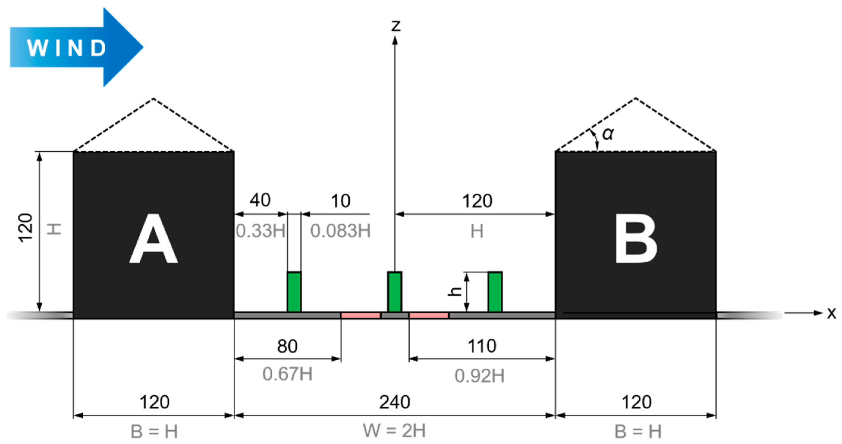
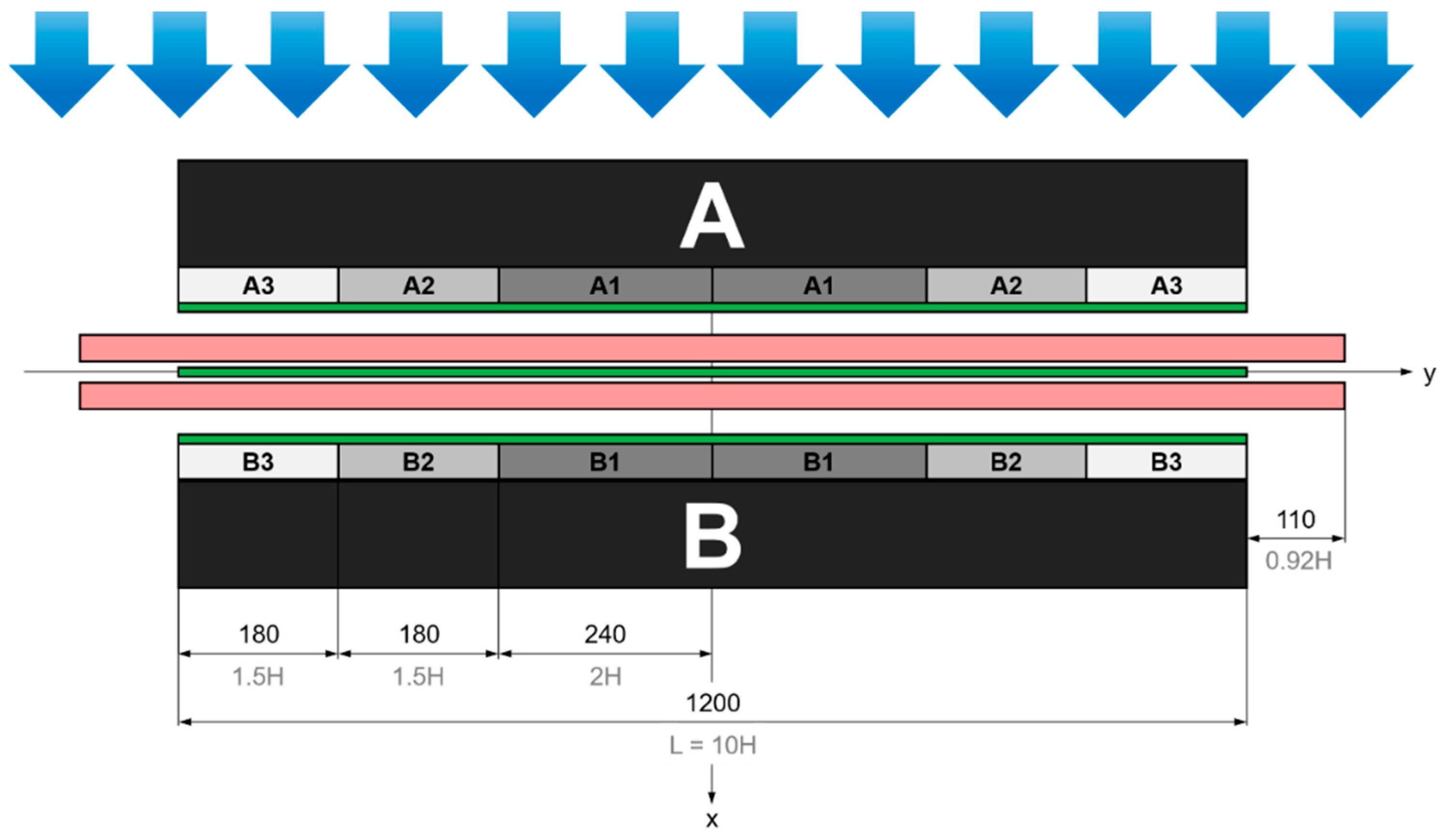
Figure 3, a generic street canyon model was formed by two parallel blocks, which consist of the leeward (A) and windward (B) buildings. Both the building height and breadth are H = B = 120 mm on both sides, and the street width is W = 2H = 240 mm. The building length (parallel to the street canyon length axis,
y) is L = 10H = 1200 mm, that is, the street canyon’s aspect ratios are W/H = 2 and L/H = 10. The geometrical parameters meet the dimensions of the reduced scale (
M = 1:150) wind tunnel model, that is, the full-scale dimensions would be the following: H* = 18 m, W* = 36 m, and L* = 180 m. Additionally, there is an option of placing sloped roofs with a roof angle α on the top of each building. The changes in the flow structure and dispersion field as a function of the roof angle has been investigated in a parameter study in the 0–50° range.
Presently, Discovery Live is not able to handle porous zones, which limits the scope of the model validation, as the effect of the hedgerows of various permeability were studied in many of Gromke’s experiments. In our investigation, low boundary walls (LBWs) were introduced in the arrangements described below.
The central boundary wall configuration (CBW) contains one low boundary wall located in the middle of the canyon, along the
y axis (
Figure 3). The sidewise boundary walls arrangement (SBW) consists of two longitudinal walls located at the opposite sides of the street canyon adjacent to the sidewalks, separating the traffic lanes from the pedestrian zones. In the case of the sidewise boundary walls, the distance between the LBW and the closest building is 40 mm. The low boundary walls have the same L = 1200 mm length as the buildings, and a width of 10 mm in all scenarios. The height of the boundary walls (
h) ranges from 0 to 45 mm (up to 0.375H) in both arrangements, including a reference scenario with no boundary walls (NBW).
As stated before, along the entire length of the buildings, two 40 mm wide areas are separated by the sidewise boundary walls on the opposite sides next to the leeward and windward walls. This width, which equals 6 m when scaled up to full-size dimensions, enables the construction of additional reduced traffic zones—such as bikeways or parking spaces—separated from the heavy traffic areas. The aforementioned areas are used mostly by pedestrians; therefore, this will be the focus area of our pollutant dispersion study, similarly to earlier investigations [
17,
19].
In order to validate the velocity field of our model, the geometrical parameters of a different street canyon defined by Gromke and Ruck [
9]—with the measured velocity data most relevant to the air exchange phenomena—were adopted. This setup is similar in size to the previously described one, except for the lack of emission zones, low boundary walls, and pitched rooftops. Furthermore, the aspect ratio of this street canyon is H/W = 1.
2.2. Computational Domain and Boundary Conditions
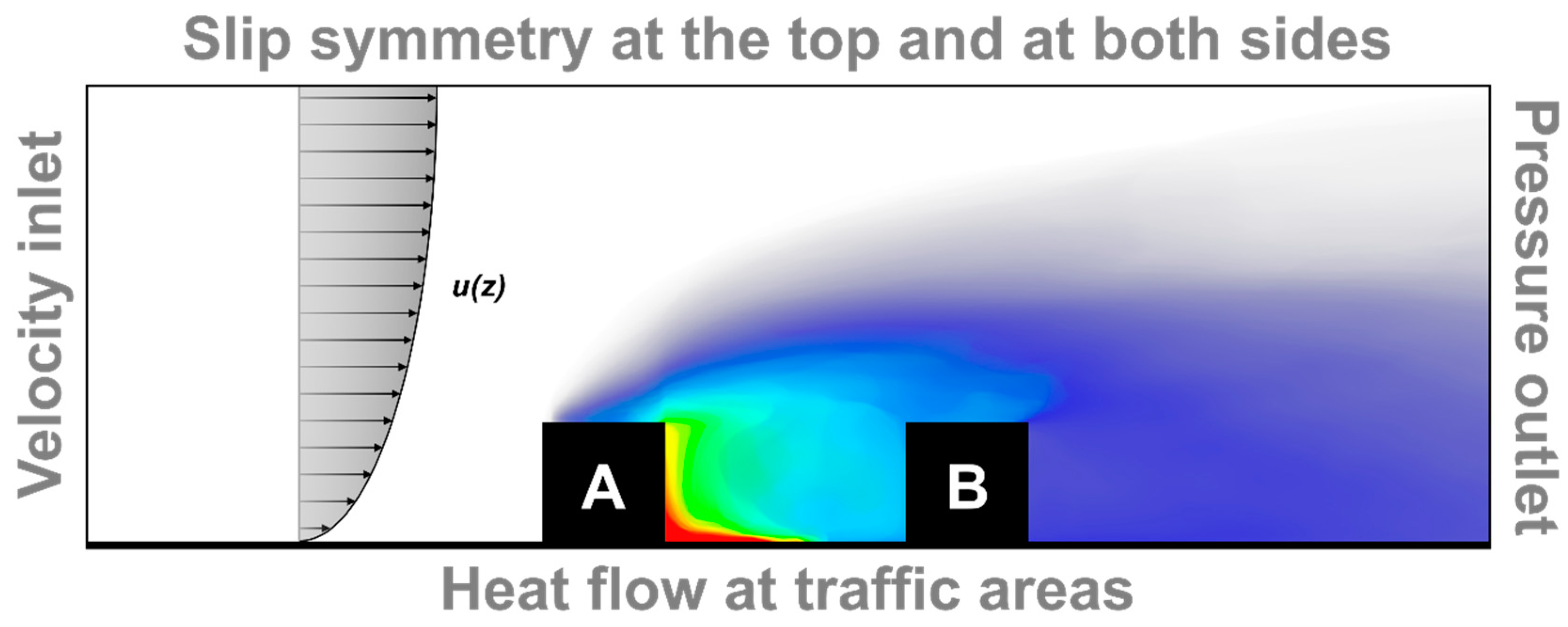
In order to reproduce the physical conditions of the wind tunnel measurements, the street canyon geometry was placed into a virtual wind tunnel using the Fluids module in ANSYS Discovery Live 19.2. The length of the computational domain is 30H, the width is 16H, and the height is 5H. The first building is located at a distance of 20H from the upstream end of the enclosure. The boundary zones of different types are indicated in
Figure 4, and are explained further in the following chapters.
2.3. Simulation of the Atmospheric Boundary Layer Approach Flow
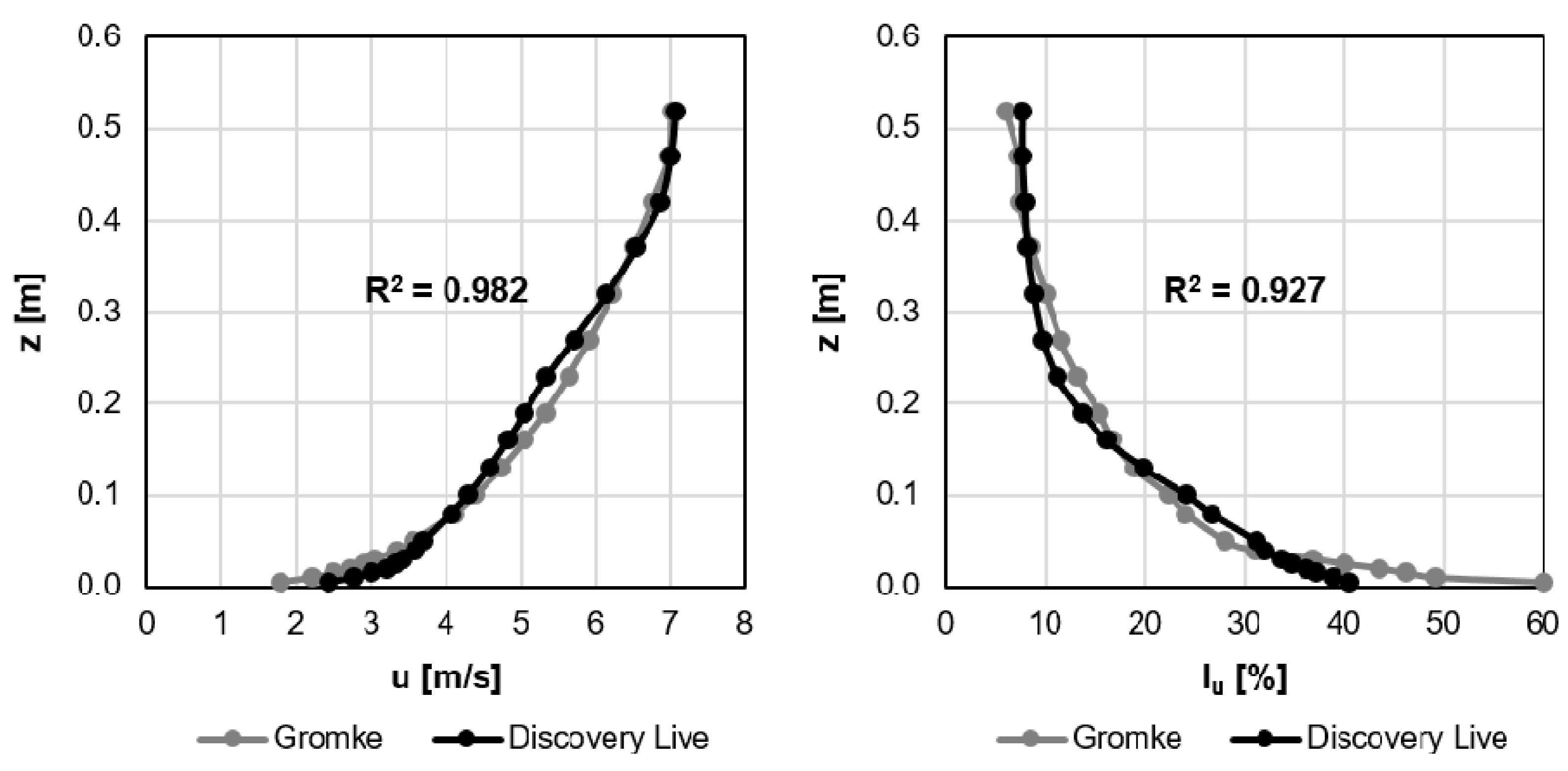
The flow approaching the street canyon in the wind tunnel [
32] is characterized by the following vertical profiles, regarding time averaged horizontal velocity (
u) and turbulence intensity (
Iu):
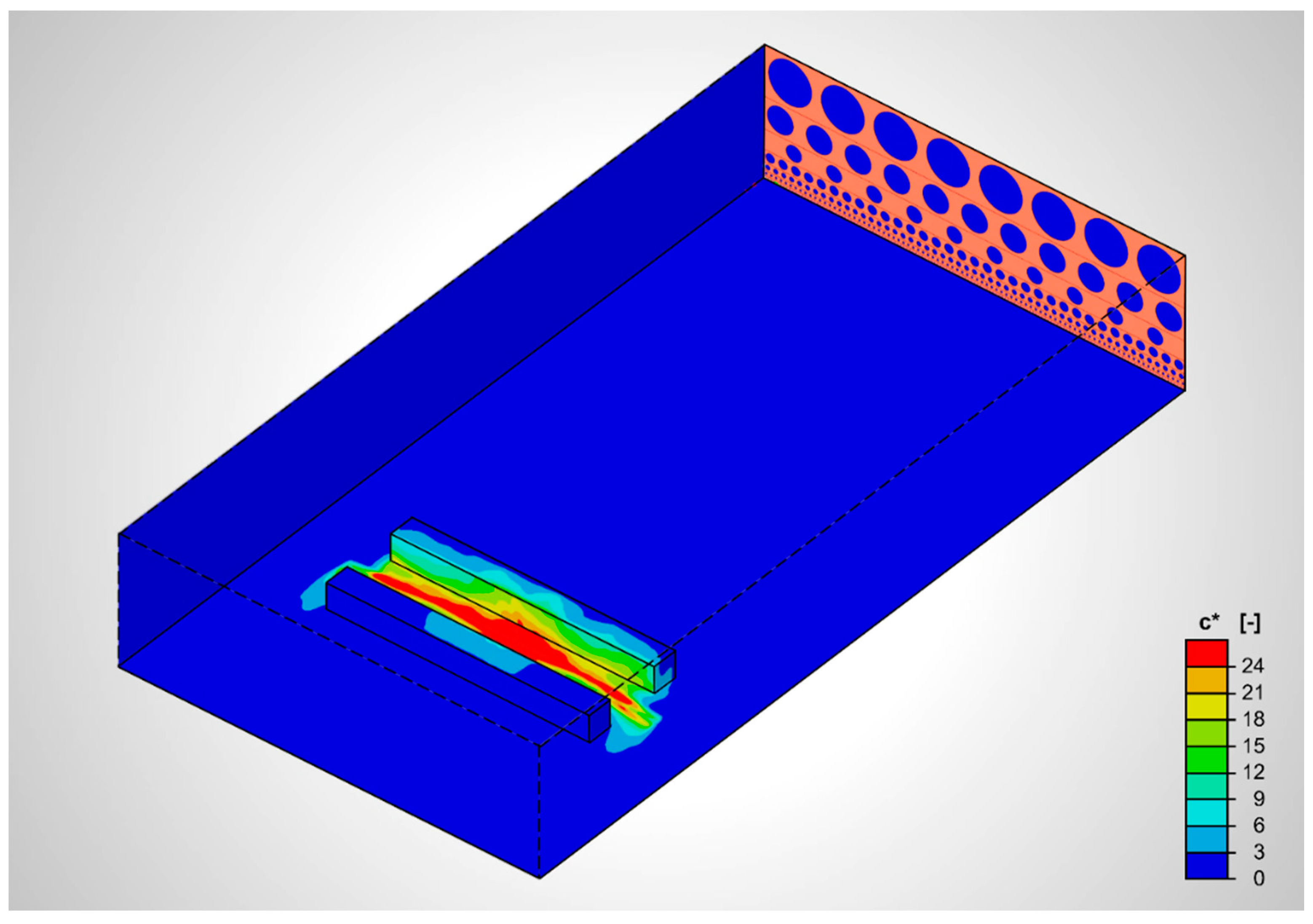
At the time that this paper is being written, Discovery Live does not allow for the specification of continuous inlet profiles; only spatially uniform, temporarily constant velocity inlets can be used. To achieve the above-described characteristics of the approaching flow, several rectangle-shaped inlets containing passive turbulence generators (circular flow obstructions) are defined on the inlet plane; as shown in
Figure 5. The height of the rectangular inlets, as well as the diameter of the circular turbulence generators grow with the distance from the ground in order to create the increasing turbulent length scale that characterizes the fully developed turbulent urban boundary layer. The number of circular cutouts in each rectangle and the inlet velocity magnitudes were fine-tuned in order to obtain the best fit both for the mean velocity and turbulence intensity in the vicinity of the street canyon. Details of the inlet configuration are given below.
The comparison between the desired and computed velocity and turbulence intensity profiles is shown in
Figure 6. The profiles realized in Discovery Live were obtained by averaging three time-averaged profiles taken in the mid-planes of three equal sectors along the
y axis (at
y/H = {−16/3; 0; 16/3}), each at H distance upstream from Building “A” (
x/H = −3). The direct output of the desired profiles is not yet available in Discovery Live, therefore 20 virtual probes were defined in the heights corresponding to the experimental setup. The probes were used to export the time series of the velocity values for post-processing.
The flow velocity at a roof level is uH = 4.636 m/s, based on Equation (1), and the reference height is H, therefore the Reynolds number is ReH = 37,000—similarly to the original wind tunnel experiment, which can be considered sufficiently high to achieve a Reynolds number independent of flow and dispersion.
It must be noted, that the parameters of the optimum inlet configuration depend on the mesh resolution, thus the values presented in
Table 1 may become sub-optimum even when the mesh is further refined. A mesh independent optimum inlet configuration would be desirable, although its development requires the perfect resolution of turbulence (DNS resolution), which is not yet feasible at the given Reynolds number.
2.4. Air Pollutant Dispersion Simulation Using Heat Transport Analogy
Presently, an arbitrary user-defined scalar transport cannot be modelled in Discovery Live; only a heat transport model is available. Therefore, a diffusion–heat transfer analogy has to be applied for modelling the pollutant dispersion process.
The analogy is based on the identical forms of the diffusive (Equation (3)) and thermal (Equation (4)) transport equations of constant property fluids supplemented with identical boundary conditions.
In Equations (3) and (4),
c denotes the mass concentration of non-settling passive pollutants in the air (kg/m
3),
t is time measured in seconds,
T (K) is the absolute temperature, while
D and
a are the diffusivity and thermal diffusivity coefficients expressed in the same kinematic unit (m
2/s), respectively. The thermal analogy requires the heat conductivity of the fluid to be chosen in a way that the Lewis number (
Le = a/
D) is in unity, therefore the fluid heat conductivity (W/(m∙K)) in the numerical model was calculated according to the following formula:
where ρ (kg/m
3) is the density, and
cp (J/(kg∙K)) is the specific heat of air at constant pressure. Note that both expansion work and viscous dissipation need to be neglected in the energy balance.
In the heat transport analogy, the temperature distribution takes the place of the air pollutant concentration field (with 0 °C indicating clear air), and the heat introduced into the model represents the rate of pollutants produced by a source.
Gromke et al. [
19] presented non-dimensional concentrations using the following definition:
where
UH (m/s) is the characteristic velocity defined at roof level,
H (m) is the building height, and
Ql (kg/(m∙s)) is the line source intensity. Correspondingly, the normalized concentration
c* was computed from the numerical model results according to Equation (7):
in which
LQ (m) is the source length and
Q (W) is the source intensity. For convenience,
Q was chosen in a way that the value of
K (1/°C) is unity, thus the Discovery Live temperature results (
T, displayed in °C units) could be directly compared with the known normalized concentration data.
In order to assess the effect of the low boundary wall (LBW) configurations on air quality in comparison to the reference scenario not containing any boundary walls (NBW), the following formula of relative concentration change was used, similarly to Gromke’s definition.
The line sources of the wind tunnel experiment—placed over the inner traffic lanes through the entire length of the street canyon, with a 0.92H long extension at each end to model the effect of the intersections—were represented in the present model by two rectangular emission zones of the same length on the inner sides of the road (indicated by the pink color in
Figure 2 and
Figure 3).
The time dependent concentration field over the pedestrian areas was monitored in two different ways. Firstly, for direct comparison, local probes were placed in the 136 sampling points of the wind tunnel measurement, and secondly, to establish the tendencies in the change of the concentration field from the effect produced by the low boundary walls, area-averaged concentration values were tracked on pre-defined surfaces during the simulation process. Following Gromke’s footsteps, the canyon floor was divided into the following areas (illustrated in
Figure 3):
Center area (|y/H| < 2.0): the area of the street canyon where the dominant flow structure is the canyon vortex (characterized by a horizontal rotational axis);
Transitional area (2.0 < |y/H| < 3.5): the area of the street canyon where the effects of both the canyon vortex and the corner eddy can be observed;
Corner/end area (3.5 < |y/H| < 5.0): the area dominated by the corner eddy (with a vertical rotational axis).
These regions were defined on the ground surface of both the leeward and windward side pedestrian zones—as averaging in arbitrary inner surfaces, for example, at pedestrian head height, is not yet possible in Discovery Live. Hence, altogether, there are six different areas to monitor using output charts, from which the time series of the area-averaged concentration can be exported. The simulation covered 20 s in physical time, and to avoid errors originating from the transient effects, only the data from 5 to 20 s was used for the statistical analysis.
2.5. The Numerical Mesh and Mesh Convergence
In ANSYS Discovery Live, the user does not have full control over the mesh properties. The software uses finite volume method with large eddy simulation, and it is capable of generating an equidistant Cartesian mesh of an automatically determined resolution. The details of the discretization schemes are not yet disclosed, however, it is known that the spatial resolution depends on the amount of on-board graphical memory, on the Speed/Fidelity ratio set by the user within Discovery Live, and on the domain size. Consequently, a tradeoff needs to be made between the discretization error, which increases with the domain size, and the model errors due to boundary influences, which decrease with the domain size.
It must be noted, that in the current version of the software, no direct information is available about the mesh size, although it can be estimated from the model outputs with acceptable accuracy, by using the below described grid interference method. Apart from the mesh resolution, the time step size is also automatically determined by the software. The model outputs presented in the Results section can be reproduced by using the same type of graphics card, which was a single NVIDIA GTX 1080Ti, or by another graphics card with at least the same amount of video memory with a properly chosen speed/fidelity setting. To the best of our knowledge, other hardware components do not influence the software’s performance.
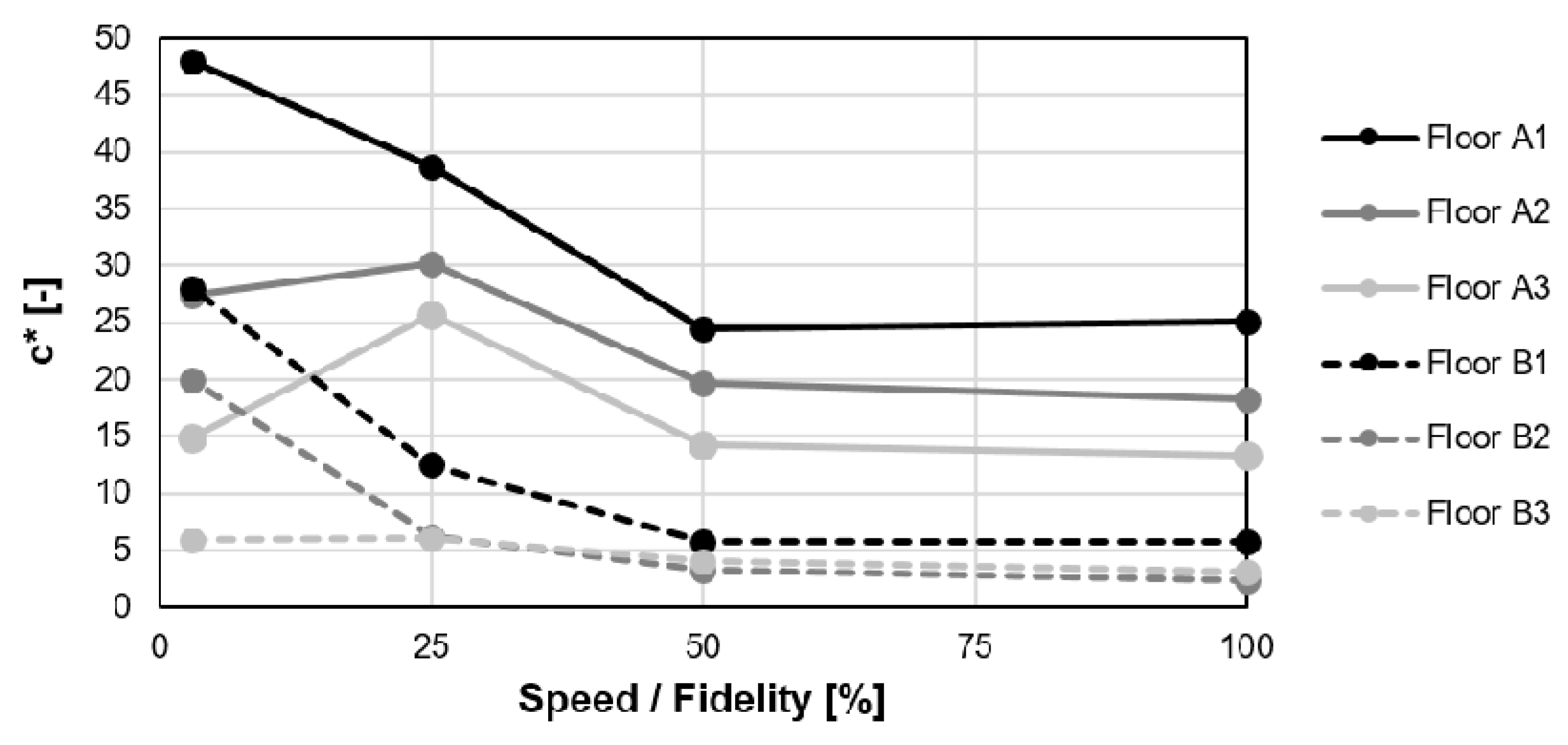
To explore the effect of the speed/fidelity parameter, the NBW reference case was run using speed/fidelity ratios of 25%, 50%, and 100%, with the latter being the finest discretization available. The normalized air pollutant concentration results from all of the six focus areas of the street canyon against the different speed/fidelity values are compiled in
Figure 7.
For estimating the mesh resolution, a staircase shaped test object was placed into the computational domain. The staircase consisted of 16 steps, each with 5 mm height and 40 mm length. As the stairs are lower than the mesh resolution, not every one of them is resolved by the mesh. By examining the streamlines while the flow simulation is running, it is possible to identify which steps are resolved (R) and which ones are skipped (S) by the mesh. The grid interference pattern can be represented by a 16-character string of R and S letters. Only a small range of mesh resolution produces exactly the same grid interference pattern, that is, by calculating the interference pattern with several hypothetic mesh resolutions, the valid range of the actual mesh resolution can be determined. Using this grid interference method, the mesh resolution could be calculated with ±0.58% accuracy at a 100% speed/fidelity ratio. The mesh details of the examined speed/fidelity cases are summarized in
Table 2.
The results of the scale resolving models change with the mesh resolution, because of both the change of the discretization error and the change of the portion of resolved turbulence; therefore, a regular mesh convergence cannot be expected. As can be seen in
Figure 7, the 50% fidelity results are reasonably close to the results produced with maximum fidelity. In Discovery Live (using the aforementioned GPU), a large eddy simulation with a 20 s long time interval can be completed in approximately an hour at 100% fidelity, and therefore the use of the finest discretization can be considered reasonable, and thus all of the dispersion cases were computed at the maximum resolution. From the model outputs, the finest spatial resolution was estimated to 7.74 mm, thus in the flow direction, the computational domain is divided into approximately 465 voxels, the height of the buildings is around 16, and the street width can be estimated for 31 cells. The average time step size was 5.2 × 10
−4 s. Based on these data and the maximum velocity (the greatest value measured in the velocity profile, see
Figure 6), the Courant number is around 0.5.
3. Results and Discussion
In our study, we focused exclusively on cases with the street canyon subjected to a perpendicular wind direction (parallel to the x axis). First, we analyzed the flow field and the air pollutant distribution of the reference scenario with no boundary walls. Furthermore—in order to validate the Discovery Live model—the concentration results of this case were compared to Gromke’s measurement results extensively, along with the comparison of the velocity field of the narrower street canyon (H/W = 1). Finally, the results of the parameter studies will be presented.
3.1. Flow Field Observed in the Reference Scenario without Boundary Walls
Being an isolated group of buildings, the flow regime around our street canyon can be described by the attributes of isolated roughness flow documented by Oke [
1]. Between the buildings, however, the characteristics of wake interference flow can be observed.
As the flow passes the leeward building, its major part is directed above the roofs, but a substantial amount also swerves around the sides of the buildings. As can be seen in
Figure 8b, a horseshoe vortex with a large recirculation zone is formed upstream from the leeward building near the ground, with the vortex axis parallel to the street canyon in front of Building “A”.
Again, as a consequence of being a sole complex of buildings, the flow above the roof of the leeward building is not entirely parallel to the ground, therefore the evolution of an approximately H long, however shallow clockwise (forward) rotating vortex, can be observed above the roof of Building “A”. These vortices described above have no direct effect on the propagation of the traffic induced pollutants in the pedestrian areas (although, the leeward side building-top vortex is able to transport pollutants upstream above the roof); the near-ground air pollutant distribution is mainly governed by the flow regime inside the street canyon.
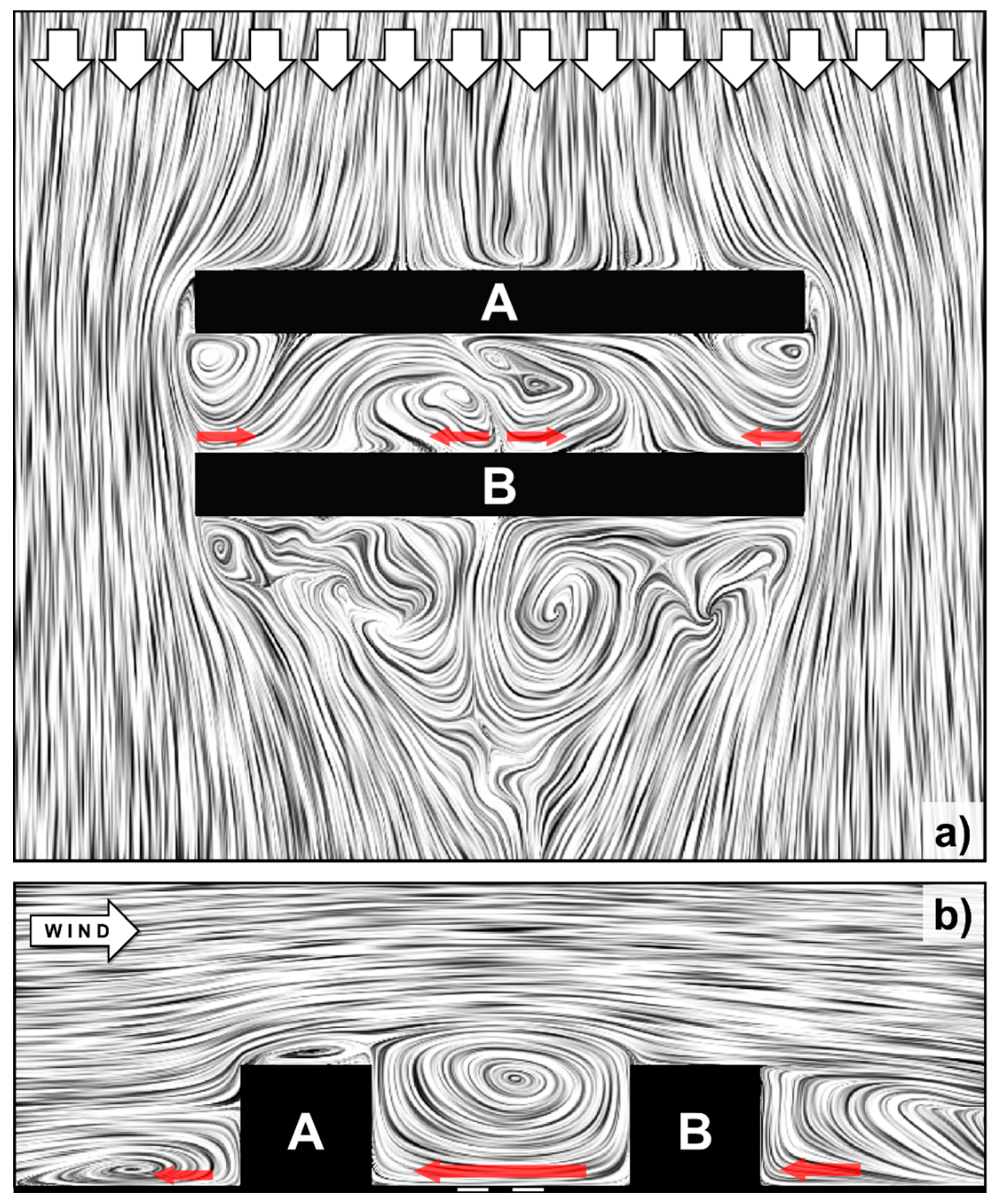
In between the leeward and windward buildings, a clockwise-rotating vortex can be observed (
Figure 8b), driven by the shear forces of the flow over the street canyon. This phenomenon was described earlier by Kastner-Klein et al. [
33], Gromke and Ruck [
9], and Gromke et al. [
19] as canyon vortex, but it can be referred to as primary vortex [
1,
34], horizontal vortex [
35], lee vortex cell [
1,
36], vortex circulation [
36], or mixing circulation [
37]. It can be observed in Discovery Live, that the vortex core is a strongly curved line throughout the length of the street canyon, similarly to the description by Kellnerova and Janour [
38], and it also loses its continuity in the instantaneous flow field. It can be seen in
Figure 8b, that the top of the canyon vortex is significantly raised above the roof of the buildings, which is one of the attributes of the wake interference flow. In the case of multiple street canyons placed one after another in an upstream and downstream of flow direction, one can expect a skimming flow to develop over the buildings [
1], which could lead to a flatter and straighter stream of air in the proximity of the rooftops.
Apart from the primary vortex, the flow field near the lateral ends of the street canyon is dominated by the effects of the air stream swerving around the sides of the buildings, which results in the formation of the corner eddies (illustrated in
Figure 8a), which have a vertical axis of rotation in contrast to the horizontal rotational axis of the main canyon vortex. The corner vortices of roughly W diameter were previously observed by Hoydysh and Dabbert [
35], Belcher [
37], Gromke and Ruck [
9], and Kellnerova and Janour [
38].
The corner eddies direct air into the canyon on the windward side and out of the canyon on the leeward side. This movement, superposed with the effect of the primary canyon vortex, which moves the air to the leeward side in the vicinity of the street surface, results in a diagonal motion pointing from both windward ends towards the center of the street canyon on the leeward side. This stream can be clearly identified in
Figure 8a.
Over the windward building, the flow attaches to the rooftop, and a large recirculation zone develops downstream from Building “B” along the entire length of the street canyon complex, and the wake of the objects can be observed even at the outlet of the virtual wind tunnel, 6H distance downstream from the actual geometry.
The phenomena described above also correspond to the CFD results by Buccolieri et al. [
14] for the same geometry.
It can be observed from
Figure 8a that the flow pattern displays some asymmetries, because the averaging time of the streamline visualization is limited in the present version of Discovery Live, although a long averaging would be necessary because of the slowly evolving vortex structure in the building wakes.
3.2. Air Pollutant Dispersion in the Reference Scenario without Boundary Walls
The typical distribution of the traffic induced air pollutants in the NBW reference case is illustrated by
Figure 5 (and later in Figure 13a,c).
The clockwise-rotating canyon vortex—depicted in
Figure 8b—transports the pollutants from the near-ground emission zones to the leeward direction. Consequently, a significant difference (with a factor of nearly five) can be observed in terms of the normalized concentration between the full area of the leeward and windward pedestrian zones (19.6 and 4.0, respectively). Based on this asymmetry, it can be concluded that the crucial area regarding the pedestrian exposure to traffic induced air pollutants is the leeward side walkway.
The corner eddies—characterized by a vertical axis of rotation—are capable of sweeping out a substantial amount of the air pollutants on both ends of the leeward footpath, thus creating a relatively clear corner section on this side. On the other hand, over the windward walkway, their effect is inverted; the vortices transport air pollutants into the canyon, resulting in a relatively contaminated corner area—compared to the transition zone on the windward side.
As a consequence of the continuous flow towards the middle section from the corners, the most heavily polluted regions are located in the center areas on both the leeward and windward pedestrian zones, with mean normalized concentrations of 25.2 and 5.7, respectively. On the leeward side, the air quality improves over the footpath, as one arrives closer to the lateral ends of the canyon, with mean normalized concentrations of 18.3 in the transitional area, and 13.3 in the end area. As stated before, on the windward side, the center area has the highest normalized concentrations as well, but it must be noted that this concentration value is lower than that of the clearest area of the leeward pedestrian zone. As discussed above, the corner eddy has an unfavorable effect on the windward side’s pollutant concentrations in the corner regions (with the mean value of 3.2), therefore the less contaminated region on the windward footpath is the transitional area, with 2.4 of mean normalized concentration.
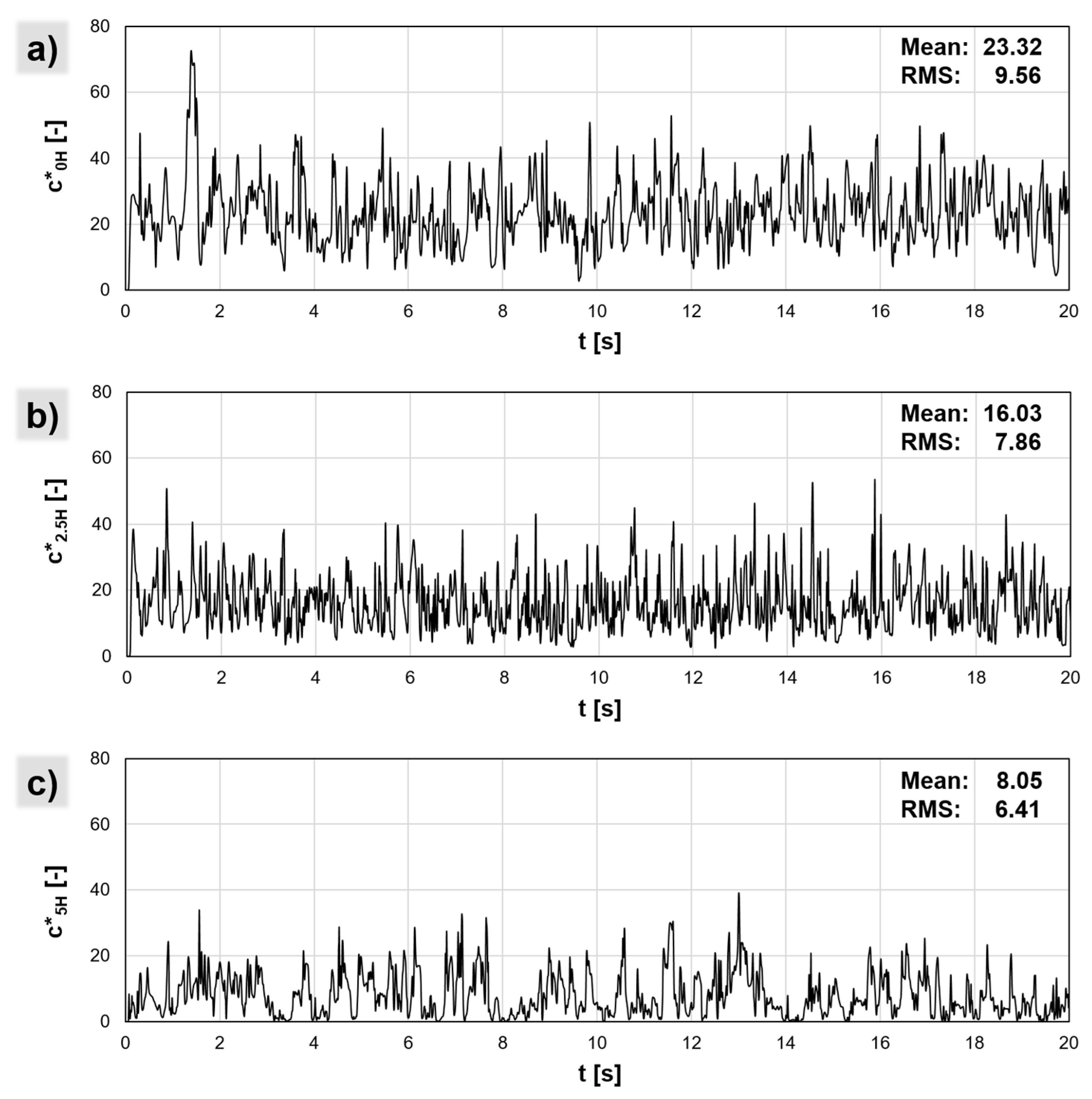
As shown by the graphs of
Figure 9, the normalized concentration displays drastic fluctuations at each point; the RMS (root mean square) value approaches the mean, and some of the peak values are three times higher than the average.
3.3. Model Validation
In the course of the validation process, the following simulation results from the Discovery Live CFD model were compared to the wind tunnel measurements:
The velocity and turbulence intensity profiles of the approaching flow of Gromke et al. [
19];
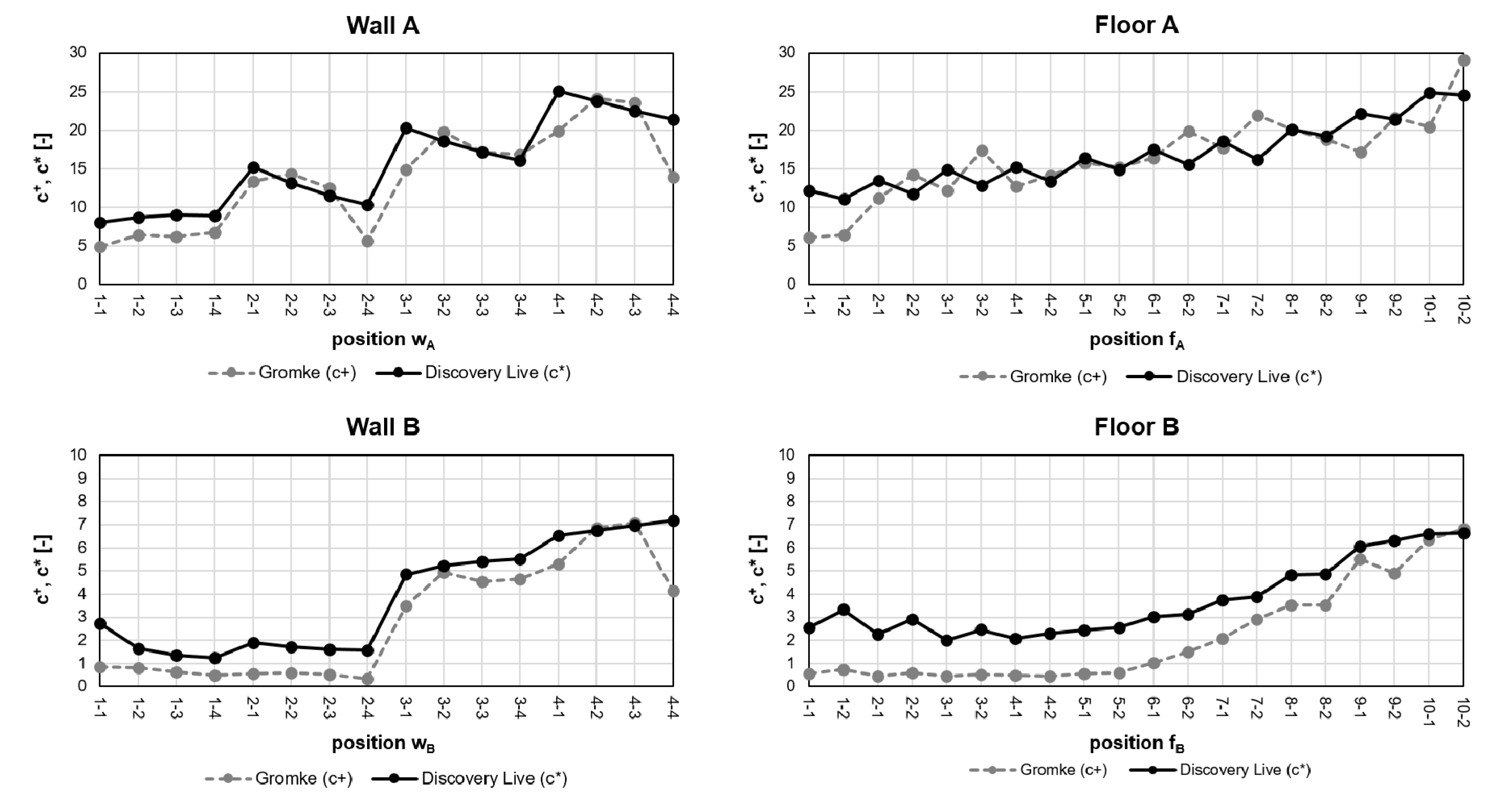
The pointwise normalized concentrations of Gromke (2016) at the Wall A, Wall B, Floor A, and Floor B measurement locations of the H/W = 0.5 aspect ratio street canyon, without the hedgerows or low boundary walls of Gromke et al. [
19];
The pointwise velocity data at the end planes and at the roof height of the H/W = 1 aspect ratio street canyon of Gromke and Ruck [
9].
As shown by the graphs of
Figure 6, with the help of the inlet configuration detailed in
Section 2.2, the desired velocity and turbulence intensity profiles (Equations (1) and (2)) could be reproduced with R
2 = 0.982 and 0.927 coefficients of determination, respectively. The deviation of the boundary layer characteristics in the wind tunnel experiment from the desired profiles is not known.
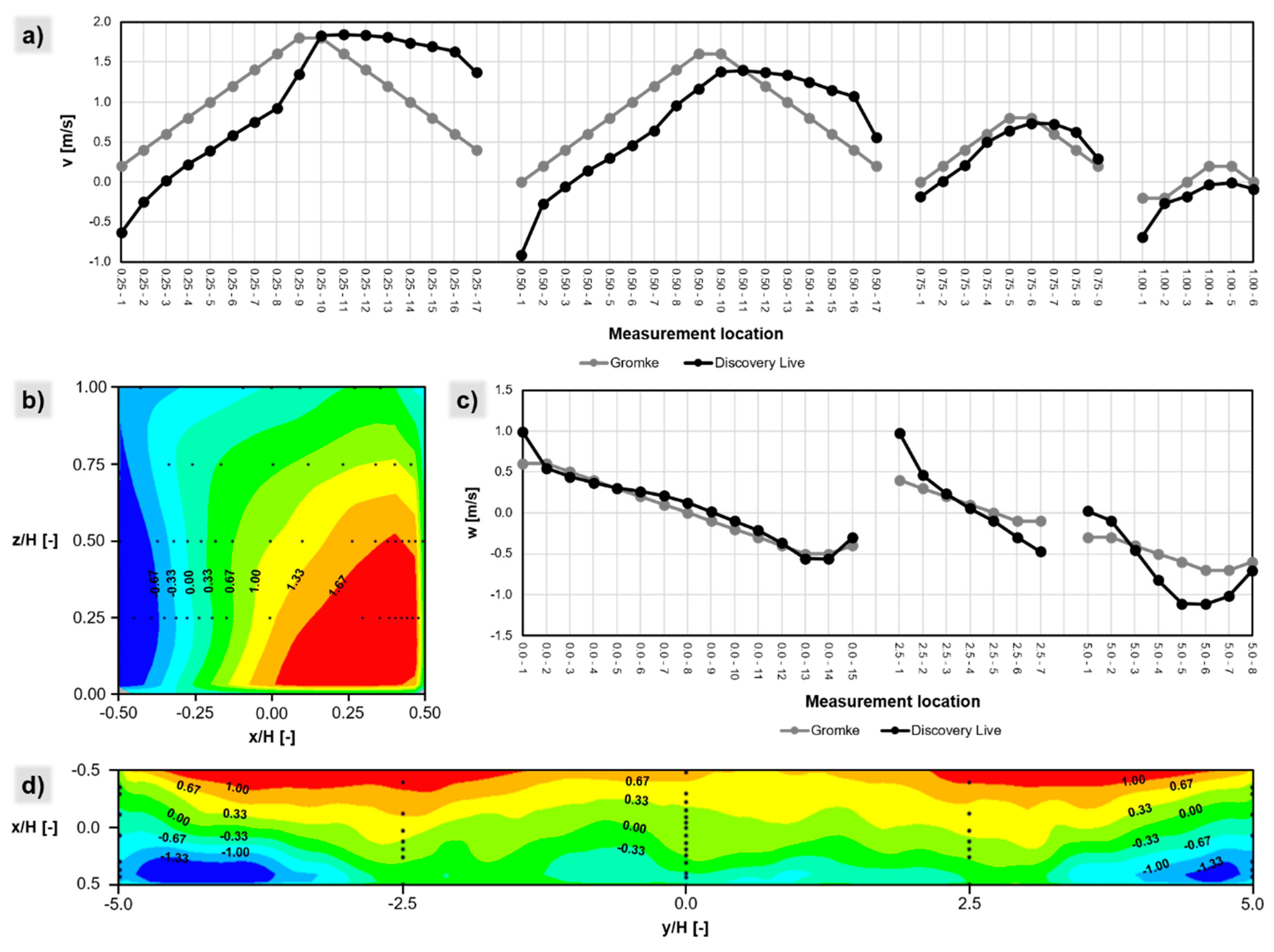
In
Figure 10, the model results are compared with the measured surface normal velocity components at the lateral and upper boundaries of the street canyon. As can be seen from the graphs, the model captures the basic flow structures, and the maximum velocities are reproduced with remarkable accuracy. Most of the deviation from the reference data is caused by the slight displacement of the maximum inflow location on the lateral sides. The coefficient of determination of the velocity dataset is R
2 = 0.697.
According to the validation criteria established by COST Action 732 [
39], the quality metrics for the normalized concentration results were calculated and listed in
Table 3.
The superior match between both the velocity and concentration results with the measurement data is partly due to the fact that the buildings being tested are sharp-cornered bodies with straight walls, which can be captured well by the Cartesian mesh of Discovery Live. Furthermore, as a consequence of the cuboid-shaped buildings, most of the flow field is not influenced by the boundary layers that develop on the surface of solid objects, which cannot be resolved by the current version of the software. The model errors can be considerably larger if the buildings to be inspected include curved surfaces.
The model shows some errors exceeding the absolute measurement error in the windward sidewall (Wall B 1.1…6.2), but the measured concentration values are relatively small in these locations. Exploring the cause of the deviation requires further investigation. Possible causes may be (A) the numerical diffusion introduced by the solution method, (B) the imperfect resolution of the turbulence spectrum, (C) the inaccuracies in the approaching wind profiles, or (D) the errors due to the reduced domain size. Unfortunately, the details of the sub-grid-scale stress model and the flux scheme are not yet disclosed by the developers; therefore, a meaningful investigation of the above causes cannot be carried out.
3.4. Air Quality Improvements by the Low Boundary Walls
As a part of the parameter studies, different configurations of central and sidewise longitudinal low boundary walls were placed in the street canyon. The height of the walls in both types of arrangements were multiples of the edge length of the equidistant Cartesian mesh (7.74 mm). Including the wall-free reference case, the dispersion analysis was carried out with 13 different LBW configurations, with a maximum full-scale LBW size of 6.97 m (0.39H). The normalized concentration results for all of the scenarios regarding the six focus areas are compiled in
Figure 12.
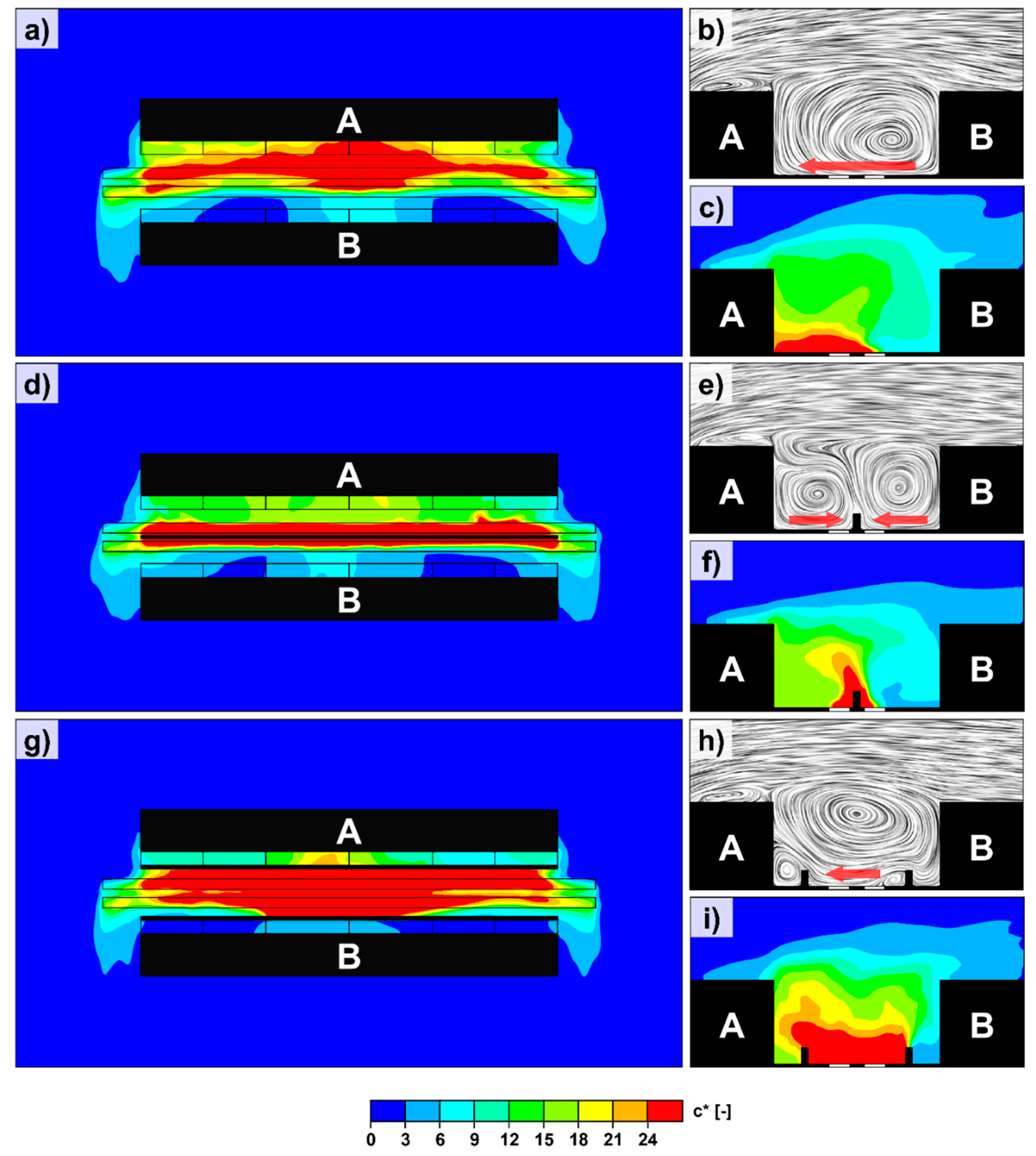
The central boundary walls—even at a height of 1.2 m—are capable of deflecting the flow headed towards the leeward sidewalk from the street surface over the emission zones. At around three meters of CBW height (or higher), the flow is routed vertically upwards, therefore enabling the formation of a counter-rotating secondary canyon vortex, of approximately the same size as the primary canyon vortex (
Figure 13e).
The consequence of the above-described phenomena is that on both sides of the central boundary wall, the near-ground flow is directed towards the middle lanes, then vertically upwards, transporting the majority of the air pollutants from the source areas to the mixing layer at the upper boundary of the street canyon. As a result, the traffic induced air pollutants are substantially diluted before reaching the crucial pedestrian areas.
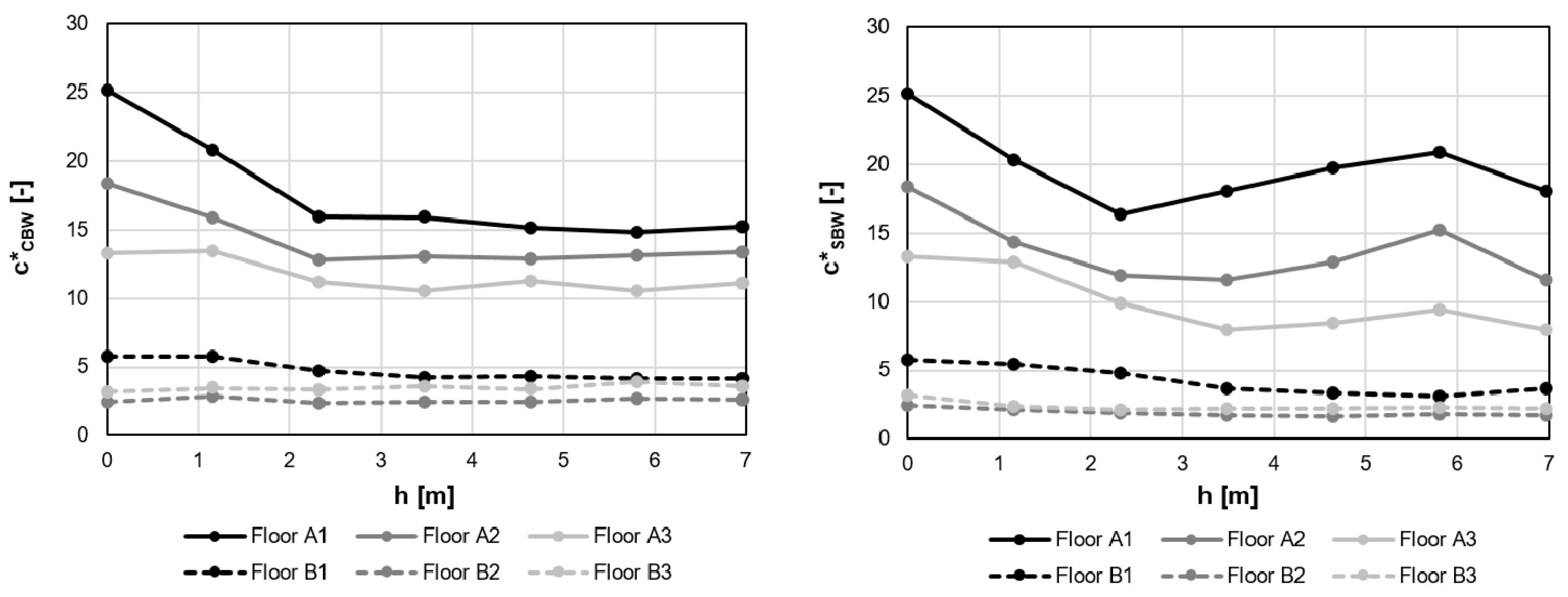
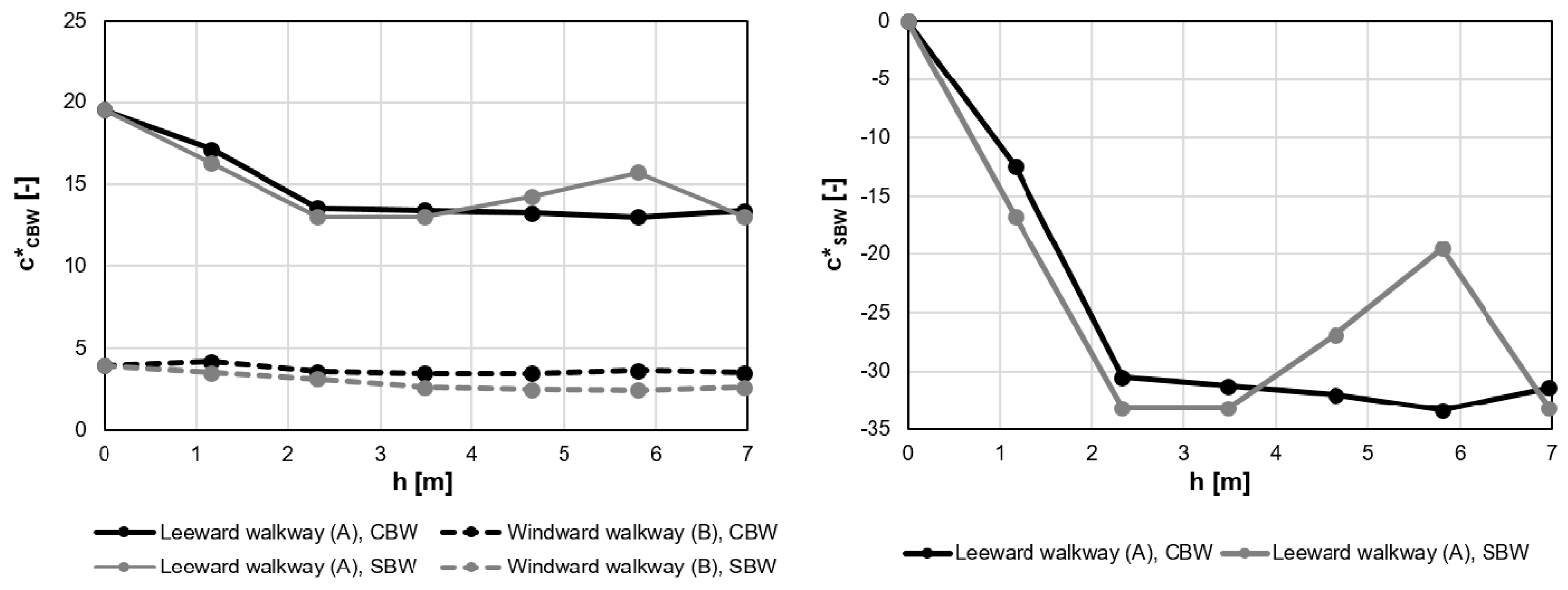
This fundamental change to the flow field causes significant differences in the concentration field. The most heavily contaminated area shifts from the leeward pedestrian zone to the inner lanes, resulting in the improvement of air quality, viz. a negative concentration change of 12.4% to 33.4% at the leeward side walkway, as shown by the graphs of
Figure 14. The concentration decrease is nearly proportional to the LBW height at the lower boundary walls; however, above two meters, the extra height results in only marginal improvements (between 30.5 and 33.4).
A minor air quality improvement is detected over the windward walkway, where the pedestrian exposure to the traffic induced air pollutants is inherently small, resulting in normalized concentration values between 3.5 and 4.2.
It is important to note, that by redirecting the flow, the CBW arrangements improve the air quality in the vicinity of both leeward and windward walls, providing the residents of the buildings with significantly cleaner air.
The sidewise boundary walls—contrary to the central boundary walls—do not restructure the flow within the street canyon. Although they modify the shape of the canyon vortex and generate two smaller eddies in their wake (shown in
Figure 13h), their main role instead is sheltering the pedestrian zones from the heavy traffic areas.
As can be seen in
Figure 14, a significant relative decrease in the normalized concentration (down to 13.1 on the leeward side) can be achieved using the SBWs of about three meters in height, reaching a relative change of −33.2% using SBWs, exceeding even the effect of the CBW with the same height. More importantly, the SBWs cannot decrease the concentration of air pollutants near the building walls as much as the CBW with the same height. Furthermore, it is worth noting that SBWs also prevent air exchange over the traffic lanes, thus increasing the average ground level concentration when the total area is taken into account. Therefore, SBWs may increase the exposure of vehicle drivers to traffic induced air pollutants, which prompts further investigation.
In conclusion, according to the present model, boundary walls with a medium height (around two to three meters) are capable of efficiently reducing pedestrian exposure to traffic induced air pollutants by one third at the critical location of the street canyon. Among the analyzed configurations, central boundary walls seem to be favorable, as they are able to decrease pollutant concentrations at the building walls, as well as at pedestrian head height on the leeward side.
3.5. The Impact of the Roof Angle
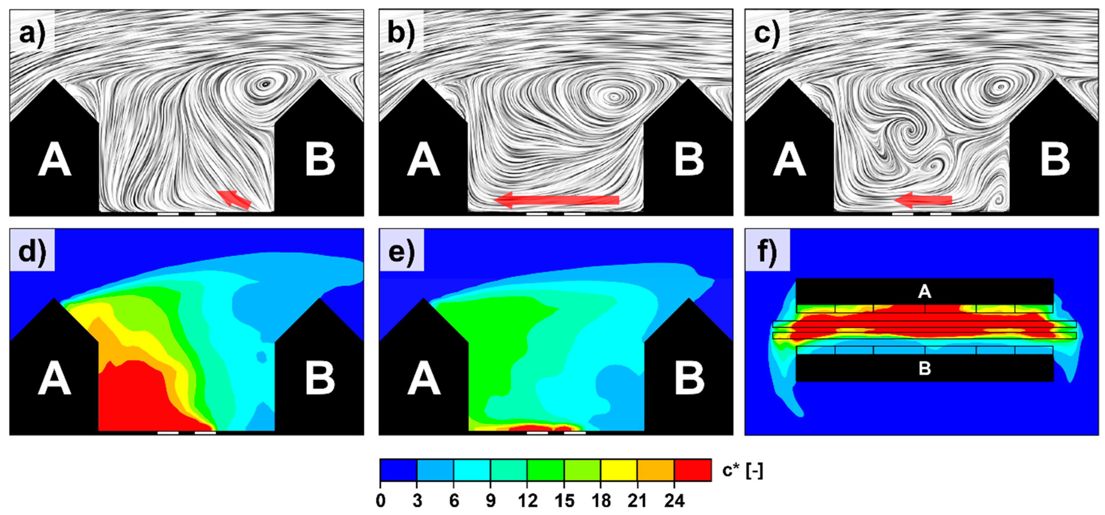
The pitched roofs placed on top of the buildings (examined in the range of slope angle α, between 20° and 50° in four separate cases) alter the flow field by shifting the core of the canyon vortex, thus generating an intense, medium-sized recirculation zone in the vicinity of the roof of the windward building. Large-scale turbulence prevailed deeper in the street canyon. The flow structure (illustrated in
Figure 15a–c) changes both spatially and temporally in the street canyon, although the advection caused by the shifted primary canyon vortex was observed along the whole length of the canyon during the entirety of the simulation.
The shift of the canyon vortex in the case of buildings with pitched roofs (
Figure 15) may depend heavily on model features such as the arrangement of crossroads or the number of successive buildings, which is confirmed by the fact that this phenomenon does not occur in the recent LES results of Kellnerova et al. [
40] obtained in a periodic computational domain featuring infinitely wide pitched roofed buildings without crossroads.
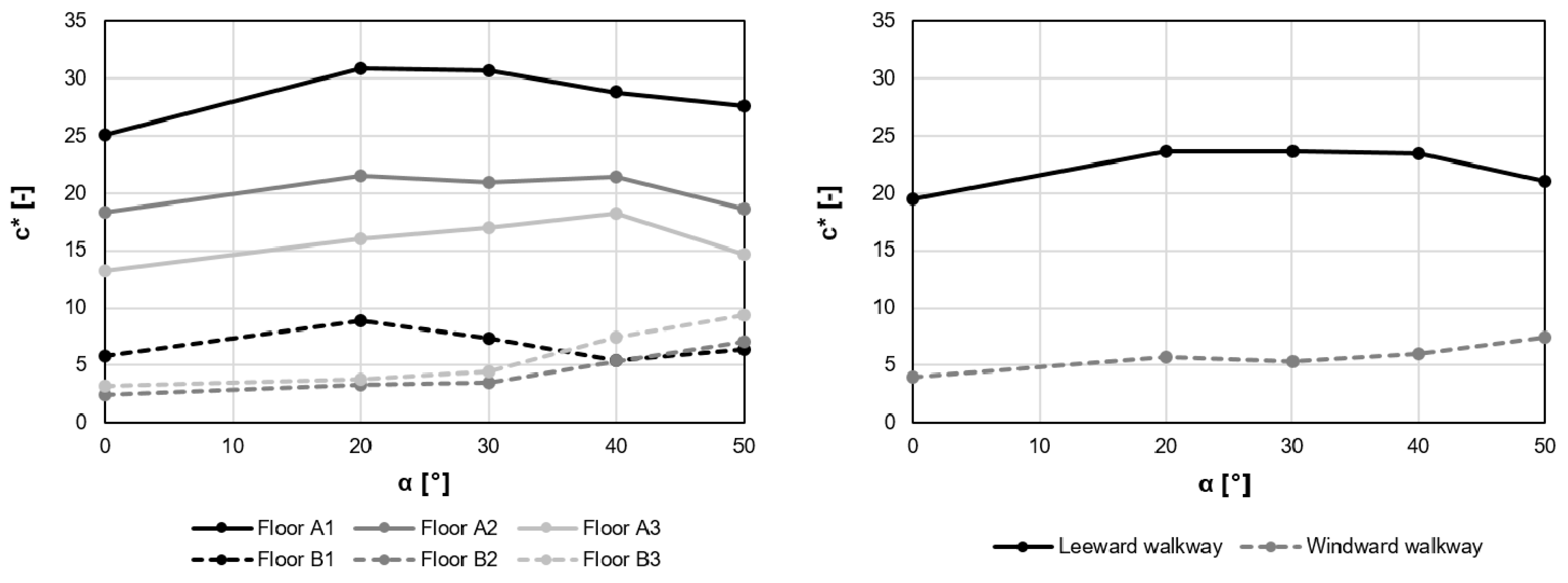
The concentration distribution within the street canyon displays a pattern similar to that of the reference case characterized by flat roofs, although the more intensive turbulent mixing tends to balance leeward and windward concentrations in the case of steeper roofs. It was observed that the leeward side mean concentration is still higher than the windward side concentration by at least a factor of three in all cases.
Figure 16 shows that the introduction of the sloped roofs, which elevates the mixing layer, causes a rise in normalized concentration over both walkways as well. However, it can be observed, that at a 50° roof angle, the leeward concentration decreases and the windward concentration further rises, that is, the extremely high pollution in the middle of the leeward sidewalk is mitigated by the enhanced mixing.
4. Conclusions and Outlook
ANSYS Discovery Live 19.2, which is primarily developed for mechanical engineering applications, seems to be a useful tool for examining the dispersion of urban air pollutants by utilizing the analogy between heat and mass transport processes. Owing to the GPU-based calculation method and automatic meshing, the large eddy simulation (LES) models can be significantly accelerated on commonly used PCs. Discovery Live can be used beneficially in the early phases of the design process for the selection of favorable concepts, which can be further examined with established CFD tools or wind tunnel experiments. With the help of this software, it was possible to produce statistically converged LES results on a PC using a NVIDIA GTX 1080Ti graphics card, in approximately one hour of computing time.
Using the inlet configuration and computational domain presented in this paper, the LES provided satisfactory agreement with the time averaged approaching velocity and turbulence profiles used in the earlier wind tunnel experiments [
19], as well as the velocity distribution of the airflow entering and leaving the finite length street canyon. The concentration distribution of the LES model showed an excellent agreement with experimental results [
19], according to the common validation metrics [
39], which suggests that Discovery Live is applicable in urban dispersion studies subject to the following conditions:
the investigated flow needs to be insensitive to boundary layer effects (e.g., only sharp-edged buildings are assumed);
the unresolved geometrical features do not substantially impact the flow; thus, the use of porous media models is not necessary;
the investigated pollutant can be well represented by a passive scalar;
the flow is isothermal;
the source intensity is pre-defined and does not depend on flow characteristics;
the investigated geometrical configuration is simple enough to allow for the resolution of every important flow feature.
In this study, the favorable effect of low boundary walls (LBWs) on the air quality of the street canyon was analyzed in a wider parameter range compared to previous studies, investigating the relationship between flow structure and concentration distribution. In the reference scenario without any boundary walls, the highest concentration of pollutants is generated at the center of the leeward pedestrian zone in the case of the street canyon subjected to wind with a perpendicular approach. Based on our model results, pedestrian exposure to traffic induced air pollution can be reduced by LBWs—or dense hedgerows—placed either in the middle of the street or between the sidewalks and the traffic lanes. The maximum achievable concentration decrease using the LBWs was about 41% at the critical point, however, over the leeward walkway, the concentration can be mitigated by one third of the inherent mean concentration, according to the present model.
From the point of view of the air quality of the sidewalks, the LBWs placed on both sides result in a similar degree of concentration reduction as that of the central LBW; however, in the latter case, the concentration increases over the traffic lanes. Both solutions require a substantial LBW height; roughly h = 0.15H is necessary in a street canyon with an H/W = 0.5 aspect ratio.
The building models used in the wind tunnel experiments of Gromke et al. [
19] were completed with pitched roofs, and the effect of the roof’s angle on air pollutant concentration over the pedestrian sidewalks was investigated. Although the lowest concentration was found in the case of flat top buildings, only a moderate concentration increase was found with a 50° roof angle, which suggests that the construction of slightly shorter buildings with pitched roofs, such as those utilized by loft apartments, could further improve air quality on the sidewalks, while retaining useful built-in volume. To explore the effects of such geometrical modifications, further investigations are planned by using the modelling approach presented.
In the authors’ opinion, the relatively simple developments listed below could significantly improve the reliability and efficiency of Discovery Live in urban dispersion simulations:
Providing direct information about mesh resolution and time step size.
Detailed descriptions of the governing equations, the turbulence model, and the numerical schemes.
The optional solution of a passive scalar transport equation.
More control of the averaging period, and the ability to set the interval length or the start and end points, which would make the analysis easier and more accurate.
Averaging on arbitrarily defined surfaces and volumes to enable the direct output of, for example, the pedestrian head height mean concentration, instead of the pointwise export.
Porous media models for taking into account the effect of vegetation or similar finely structured flow obstructions.
As the impact of urban architecture on the propagation of air pollutants is still largely unexplored, it is necessary to study a wide variety of different geometrical configurations. We believe that, due to its superior cost–benefit ratio, the proposed GPU-based simulation method can be an effective component for such investigations.


