Article

An Investigation of the Quantitative Correlation between Urban Morphology Parameters and Outdoor Ventilation Efficiency Indices

1
School of Architecture and Urban Planning, Nanjing University, Nanjing 210093, China
2
Dipartimento di Scienze e Tecnologie Biologiche ed Ambientali, University of Salento, S.P. 6 Lecce-Monteroni, 73100 Lecce, Italy
*
Author to whom correspondence should be addressed.
Atmosphere 2019, 10(1), 33; https://doi.org/10.3390/atmos10010033
Submission received: 26 July 2018 / Revised: 7 January 2019 / Accepted: 12 January 2019 / Published: 16 January 2019
(This article belongs to the Special Issue Recent Advances in Urban Ventilation Assessment and Flow Modelling)

Abstract

:
Urban outdoor ventilation and pollutant dispersion have important implications for urban design and planning. In this paper, two urban morphology parameters, i.e. the floor area ratio (FAR) and the building site coverage (BSC), are considered to investigate their quantitative correlation with urban ventilation indices. An idealized model, including nine basic units with FAR equal to 5, is considered and the BSC is increased from 11% to 77%, generating 101 non-repetitive asymmetric configurations, with attention to the influence of plan density, volume ratio, and building layout on ventilation performance within urban plot areas. Computational Fluid Dynamics (CFD) simulations are used to assess the ventilation efficiency at pedestrian level (2m above the ground) within each model central area. Six indices, including the air flow rate (Q), the mean age of air (τP), the net escape velocity (NEV), the purging flow rate (PFR), the visitation frequency (VF), and the resident time (TP) are used to assess the local ventilation performance. Results clearly show that, fixing the FAR, the local ventilation performance is not linearly related to BSC, but it also depends on buildings arrangement. Specifically, as the BSC increases, the ventilation in the central area does not keep reducing. On the contrary, some forms with low BSC have poor ventilation and some particular configurations with high BSC have better ventilation, which indicates that not all high-density configurations experience poor ventilation. The local ventilation performance can be effectively improved by rationally arranging the buildings. Even though the application of these results to real cities requires further research, the present findings suggest a preliminary way to build up a correlation between urban morphology parameters and ventilation efficiency tailored to develop a feasible framework for urban designers.

1. Introduction

The urbanization process in the past few decades has accelerated the increase of urban density, which leads to significant differences between urban morphology and original form in natural conditions (such as number of streets, height of buildings, void spaces, etc.). Due to the compact urban spaces, air pollutant cannot be diluted and dispersed in time, causing a series of health problems [1]. With this rapid expansion of cities, especially for some developing countries, the relationship between the urban building density and the urban local wind environment has increasingly become the focus of attention. The density and morphological characteristics of buildings play an important role in the local ventilation performance and the dispersion of pollutants. Especially, in central space that is surrounded by buildings with a high density of pedestrians, the ventilation performance is very important for their comfort and health.
Urban outdoor ventilation related to urban morphology can be assessed by full-scale field measurement, reduced-scale wind-tunnel or water channel experiment, and Computational Fluid Dynamics (CFD). With regard to full-scale field measurement, it depends on the meteorological conditions and sufficient measurement points to cover the areas with pivotal turbulence characteristics, especially for a large district [2,3]. Reduced-scale experiment and CFD can provide a controllable initial and boundary conditions [4]. However, wind-tunnel and water channel experiments are limited by the numbers and density of selected positions in order to gain the whole characteristics of flow field. When compared to reduced-scale experiments, CFD allows for providing the whole flow field data within the cells of the computational domain. Especially in recent years, with the turbulence models, computational resources and the development of best practice guidelines continued to increase [5,6], CFD has gradually become a widely used method to evaluate urban ventilation and pollutant dispersion. However, validation and verification are critical concerns for assuring the accuracy and the reliability of CFD simulations [7,8].
In the past 20 years, a large substantial series of ventilation efficiency indices have been proposed, validated, and applied to assess the local outdoor wind environment of urban areas. Ventilation indices initially developed and applied for indoor air quality [9,10,11,12], such as local mean age of air, air change rate, air exchange efficiency, purging flow rate, visitation frequency, and the residential time, were extended to predict outdoor urban ventilation [13,14,15,16,17]. The local mean age of air (τP) implies the time that one air particle reaches the given point in the specific domain after entering the flow field. A low value of local mean age of air illustrates well pollutant removal capability and a lower pollutant concentration within urban canopy layer The air change rate (ACH) refers to the frequency with which a given canopy volume of air is completely replaced by “fresh” air, and the air exchange efficiency (εa) denotes the efficiency of flushing the street network with external air. A high level of the two indices implies that much fresh air flushes the given volume and a better wind ventilation performance. The purging flow rate (PFR) quantifies the capacity that the pollutant is completely removed from a specific volume (i.e. the canopy layer) and a lower value indicates poor ventilation within the canopy. The visitation frequency (VF) is the number of times that a pollutant enters the domain and passes through it [13]. A high visitation frequency indicates high level pollutant concentration. Finally, the residence time (TP) is the time that a pollutant takes from once entering or being generated in the domain until leaving the domain [18]. While the above mentioned indices have been originally proposed to evaluate indoor air quality, other indices proposed directly for the urban street canyon model and asymmetric real city model are the exchange velocity, the pollutant exchange velocity, the net escape velocity, and the air delay [19,20,21,22,23,24,25,26]. The exchange velocity (ue) and the pollutant exchange velocity (ue,pollutant) focus on the turbulence diffusion between the in-canopy and above-canopy flows. They parametrize the mean convective exchange fluxes at the rooftop level and are usually related to the so called “city breathability”. Based on the concept of PFR in urban areas, the net escape velocity (NEV) was proposed to reflect the net pollutant removal capability from the specified volume by mean flow and turbulence diffusion. The air delay (τd) is a recent optimization measure that is independent of the initial values, as it presents the amount of time delay that is caused by the presence of the urban geometry in each point inside the domain [26].
By employing some or a combination of the above indices, several studies have investigated the relationship between geometric parameters and ventilation efficiency [21,27,28,29,30,31]. Various studies focused on idealized urban models and real-complexity urban models of different planar area density (λp) and frontal area density (λf) [16,24,32,33]. However, for urban designers and planners, key factors also involve economics, policy, and urban development strategies. In this perspective, in the early planning stage the floor area ratio (FAR) of urban plot is determined first, and the relationship between building site coverage (BSC) and ventilation performance in a specific area is evaluated [34]. Kubota et al. [35] collected the building coverage ratio (BCR, means BSC in this paper) and the FAR of 22 actual Japanese cities and used wind tunnel experiments to explore the relationship between BCR and wind velocity ratio. Results have shown that the average pedestrian-level wind velocity can be explained well by the BCR rather than by the FAR. Moreover, the FAR and the BSC have been employed by previous research to investigate the relationship between urban fabric and outdoor wind environment, especially in high-density urban areas [33,36,37].
Within this context, the two urban morphology parameters FAR and BSC are here considered to investigate their quantitative correlation with six urban ventilation indices. An idealized model, including nine basic units with FAR equal to 5 is considered; the BSC is increased from 11% to 77% generating 101 non-repetitive asymmetric configurations. Computational Fluid Dynamics (CFD) simulations are performed to assess the local ventilation efficiency at pedestrian level within each model central area. Here, the pedestrian level is taken at z = 2 m, as commonly employed in previous ventilation studies [13,15,24,26,38,39,40,41].

2. Methods

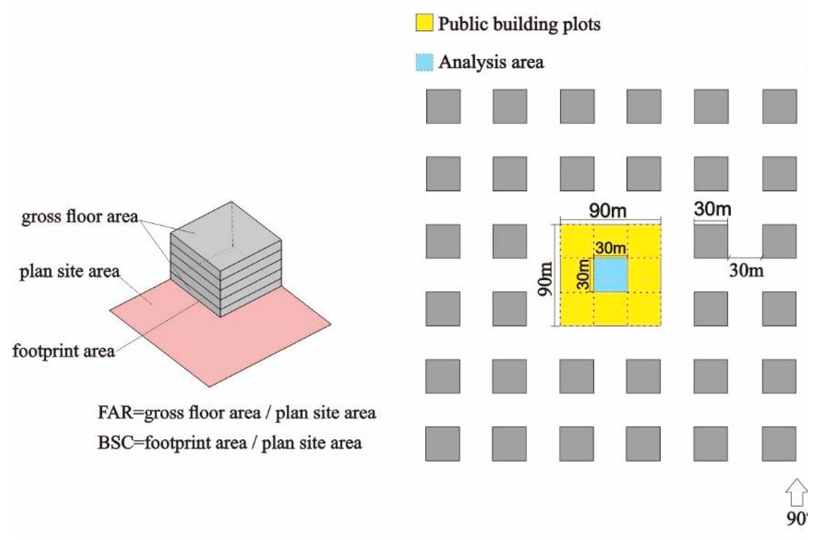
2.1. Description of Urban Blocks Morphology Characterists

As mentioned in the Introduction, during the early stage of urban planning and design, the floor area ratio (FAR) is usually fixed, being closely related to costs, benefits, development strategies, etc. The main factors affecting the morphology include the building site coverage (BSC) and the architectural arrangement. FAR represents the ratio between total floor areas and lot area, as indicated in Figure 1, which also shows the definition of BSC.
Here, an idealized model consisting of nine basic units in the plot area is considered, where each unit size is a 30-meter square. The central square (unit) is the area that cannot be covered by buildings (“central area” hereinafter) and is the area where the ventilation indices are calculated, while the other eight units surrounding the central area may be covered by buildings. FAR is fixed to 5, and the initial BSC is 11%, meaning that there is only one high-rise building. Meanwhile, there are five possibilities for the position of building in the whole plot area (excluding symmetry conditions). The central area represents a typical square that is surrounded by buildings of different height and arrangement. Ventilation in this area is worth of investigation since people spend more time here than in streets.
Thus, in order to explore the correlation between morphology and ventilation performance of the central area, all possible configurations in the plot area are considered, as shown in Figure 2. According to the architectural layout around the central area, the model is divided into “C form” and “B form”. The C form means that the front and back directions of the central area are not blocked and a channeling effect is expected. The B1~B3 form means the number of buildings along the windward projection. The B(F1~F3) form means the number of building front (in the first two rows) along the windward projection. An approaching wind direction perpendicular to building façades is considered, as it is commonly associated with the worst scenario, leading to high pollution levels around the single building, in street intersections, and in the perpendicular streets [42,43]. As a consequence, the symmetrical configurations along the east-west direction are excluded. When BSC increases from 11% to 77%, 101 different asymmetrical configurations are generated in total. Please note that the building height diminishes moving from BSC=11% to 77%, specifically they are 135 m, 69 m, 45 m, 36 m, 27 m, 24 m, and 21 m, respectively.
Conceptually, BSC is similar to λp. Here, BSC is employed in conjunction with FAR that limits the volume plot ratio, as typically done when a new building arrangement has to be built in China. Even though in the literature there are several studies relating λp to ventilation performance (see the Introduction), here we recognize that actually many possible combinations are available for the same λp (and thus BSC) for a given urban plot. Further, in Chinese cities, such as Nanjing, even in dense commercial plots, there are still some multi-storey or low-rise buildings surrounding the high-rise buildings. In this case, the corresponding urban texture becomes quite fuzzy. In this case, λp and λf may not clearly quantify the urban morphological characteristics of the fuzzy urban slice. With the morphological complexity, such as lift-up, road network inside the plot, etc., more parameters might more clearly describe the morphological characteristics of a specified area, such as FAR and BSC employed here. Finally, here we analyze the ventilation performance using six different ventilation indices (described below) and attempt to provide some suggestions about the indices that mostly correlate with urban morphological parameters.
The ventilation of the whole area, i.e. the city potential of removing pollutants and other scalars, is determined by the resistance generated by buildings, which usually implies that flow through the city downstream exit is lower than that entering the city upstream [16]. This is due to the drag force generated by the whole arrangement of buildings and cannot discriminate the single building [44]. From a practical and architectural perspective, the cases analyzed here mimic a real situation that an urban planner is faced with when a lot area of a given (fixed) size and FAR is allocated to the development of new built areas, where BSC and layout have to be chosen to optimize the ventilation.
We underline that idealized geometries have been here considered here to better isolate and elucidate the effect of changing BSC and building layout on ventilation and to evaluate the sensitivity of six different ventilation indices.

2.2. Description of the Outdoor Ventilation Efficiency Indices

The six ventilation indices employed to evaluate the ventilation in the central area are briefly described below.
The flow rate ( Q ) represents the capability of pollutant dilution through street openings and its roof by wind flow [15]. It is defined as:
Q = A 0 u ¯ d A 0
Flow rates through street openings and roof are normalized by a reference flow rate ( Q ) (the flow rate far upstream through the same area of the windward opening), as follows [15]:
Q = A 0 u ¯ d A 0
Q * = A 0 u ¯ d A 0 / Q
where Q * is the normalized flow rate, u ¯ and u ¯ is the horizontal (stream-wise) velocity along the x direction and that far upstream, and A 0 is the area of street opening.
The purging flow rate (PFR) is the net flow rate by which the specified volume is purged out of pollutant [10]. If passive pollutants are uniformly released in the entire pedestrian volume (in our case, it is fixed and corresponds to the volume from the ground to the pedestrian height of the central area), the pedestrian purging flow rate (PFRped) is defined as:
P F R p e d = S c × V o l C = S c × V o l V o l C d x d y d z / V o l
where Sc means the uniform pollutant generation rate (kg/m³·s), 〈C〉 is the spatially averaged concentration in the entire pedestrian volume (kg/m³), and Vol is the entire pedestrian volume (m³). The normalized P F R p e d * is:
P F R p e d * = P F R p e d / Q
The net escape velocity NEV is based on the concept of PFR and has been proposed by Hang et al. [17]. NEVped represents the net capacity of removing/diluting pollutant from the entire pedestrian volume by both mean flow and turbulent diffusion and it is defined as:
N E V p e d = P F R p e d A 0
where A 0 is the area of boundaries for the entire pedestrian volume.
In addition to the level of the pollutant concentration, the pollutant behavior within the domains is also important for local ventilation assessment [13]. The visitation frequency (VF) is, in this sense, an index to measure the pollutant behavior. The VF can be calculated as:
V F = Δ q p S c × V o l
where Δ q p is the inflow flux of pollutants into the domain (kg/s). It is assumed that the inflow flux in the street canyon is almost exclusively affected by the value of the mean part of the flux [13].
The residence time (TP) is the time that it takes once a particle enters or is generated in the specified domain until it leaves there. Similar to VF, the residential time represents the time that pollutant enters or is generated in the street canyon. It is defined as:
T P = V o l P F R p e d × V F
The age of air represents the mean time requiring the inflow air to reach a certain point in the specified volume. Currently, it is commonly employed to assess the ventilation efficiency of urban built-up areas [15,32,34,45]. The local mean age of air ( τ ¯ p ) can be calculated by:
τ ¯ p = c ¯ S c
where c ¯ is the local pollutant concentration (kg/m3). The local mean age of air can be normalized, as follows:
τ ¯ p * = τ ¯ p × Q r e f V o l r e f
where V o l r e f (m3) is the entire pedestrian volume.

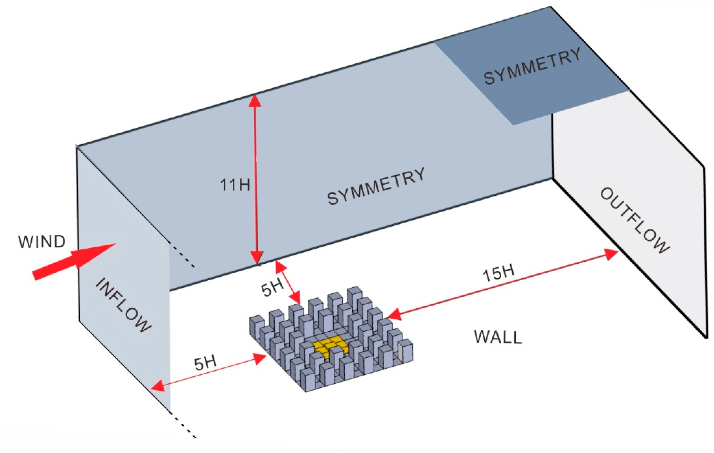
2.3. CFD Simulations Set-Up

2.3.1. Computational Domain and Grid

The computational domain was built using hexahedral elements, with a finer resolution within the entire building area (the expansion rate between two consecutive cells was below 1.2). The influence on the predictions of the choice of grid size, using several refined meshes, was verified (see the Supplementary Material S1). Specifically, the minimum cell size were δx = 0.8 m, δy = 0.8 m, δz = 0.5 m in the plot area, which means that at least three cells were present up to pedestrian level and at least 10 cells per cube root of the building volume and 10 cells per building separation, as suggested by [5,6]. The lateral and inflow boundaries were set to 5H away from the building groups. In order to unify the computational domain size, we set H = 135 m, which corresponds to the highest building of BSC = 11%. The outflow boundary was 15H away from the building groups, and the height of the computational domain was 11H. Extra 30 m high buildings were considered around the central area. The grid resolution and the computational domain size fulfill the major microscale simulation requirements recommended by the AIJ (Architectural Institute of Japan) guidelines [6] and the COST action 732 [5]. The computational domain is shown in Figure 3.
We are aware that the surrounding buildings affect the flow field before reaching the central area. These buildings have been included to explicitly reproduce roughness elements and thus the real effects of urban elements (whose height is typical of eight to ten-story buildings in China), avoiding considering an isolated central area that does not represent a real situation. For this reason, we think that the results presented in Section 3 are representative of the effects of urban-like geometries on flow, ventilation, and pollutant concentration.

2.3.2. Turbulence Model

For the choice of turbulence model, the standard Reynolds-averaged Navier–Stokes (RANS) and Large Eddy Simulation (LES) are most commonly compared and discussed in urban ventilation simulation. The accuracy of LES has been determined in adequate studies, especially in predicting the flow and turbulence characteristics in low wind speed region [25,46,47,48]. When compared to LES, the limitation of steady RANS method has been reported in many literature studies [49,50,51,52]. However, the computational cost of the LES model is several times higher than that of the RANS model. Meanwhile, RANS approach is still the most commonly approach of urban ventilation assessment, and it has shown good results for generic urban configurations [6,13,15,16,17,27,36]. For the purpose of this study, the employed RANS approach with the k-ε turbulence model is considered appropriate in comparison with other turbulence model, such as Large Eddy Simulations (LES), especially since the interest is on mean values ([53]). To further evaluate the standard k-ε turbulence model employed here, a validation study has been performed and results are presented in the Supplementary material S2.

2.3.3. Boundary Conditions and Solver Settings

For the inflow boundary conditions, the inlet profiles for U(z), k(i) and ε(z) in the atmospheric boundary layer follows the COST recommendation presented by Richards and Hoxey [54].
The velocity profile (U) was:
U ( z ) = u A B L * κ ln ( z + z 0 z 0 )
where u A B L * is the atmospheric boundary layer friction velocity, z 0 is the aerodynamic roughness length, z is the height coordinate (m), and κ is the von Karman constant (0.4). Taking Nanjing as an example, we set z 0 = 0.4, which may represent woodlands within and surrounding the city [55], and a wind speed equal to about 2 m/s at 10 m, which roughly corresponds to the 10th percentile of the mean hourly wind speeds (https://weatherspark.com/y/132872/Average-Weather-in-Nanjing-China-Year-Round) and it is expected to lead to poorer ventilation conditions than larger wind speeds. These values lead to a friction velocity equal to 0.23 m/s, which is typical of isothermal conditions analyzed here. In this way, we represented a change of surface roughness (smooth–rough) mimicking the transition from the rural to the urban environment. The turbulent kinetic energy profile (k) and turbulent dissipation rate profile ( ε ) were:
k ( z ) = u A B L * 2 C μ
ε ( z ) = u A B L * 3 κ ( z + z 0 )
where C μ is a constant (0.09). Zero static gauge pressure condition was defined as the outflow boundary condition. At the top and lateral boundaries of the computational domain, the symmetry boundary conditions were applied to avoid the wall effect. Non-slip wall boundary conditions were set on the ground surface and all of the building surfaces.
The passive pollutant used is carbon monoxide (CO, Sc = 10−5 kg m−3 s−1) and the pollutant source is defined as a volume source from the ground to pedestrian height (i.e., from z = 0 to z = 2 m) of the central area using the uniform homogenous method that was widely employed in evaluating ventilation efficiency of urban canopy layers [56].
Fluent (version 15.06) was applied to solve three-dimensional (3D) steady RANS equations for incompressible and isothermal flow. Pressure interpolation was in second order accuracy. For both convection and viscous terms of the governing equations, second-order discretization schemes were used. The modeling settings are summarized in Table 1.

3. Results and Discussion

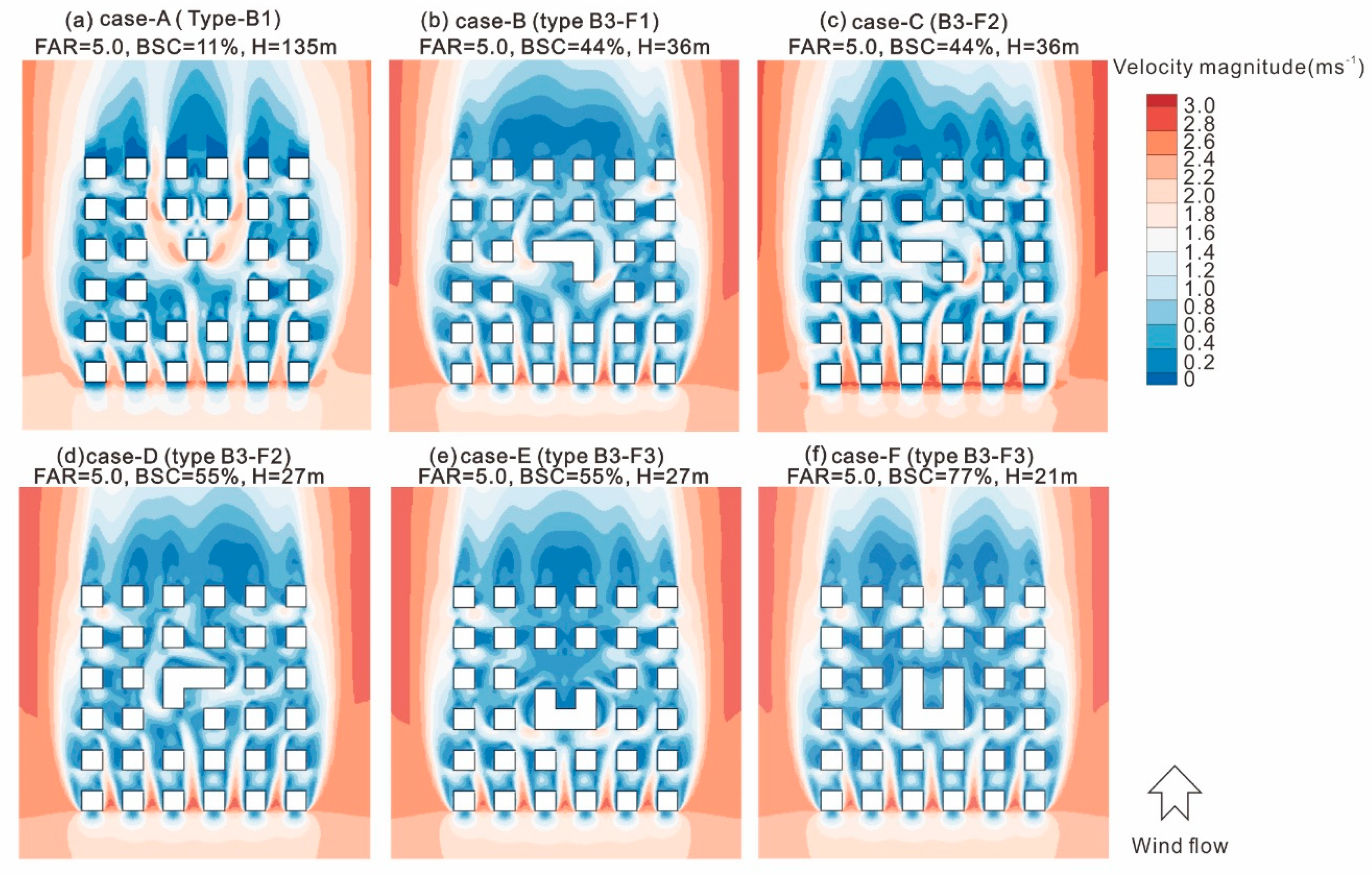
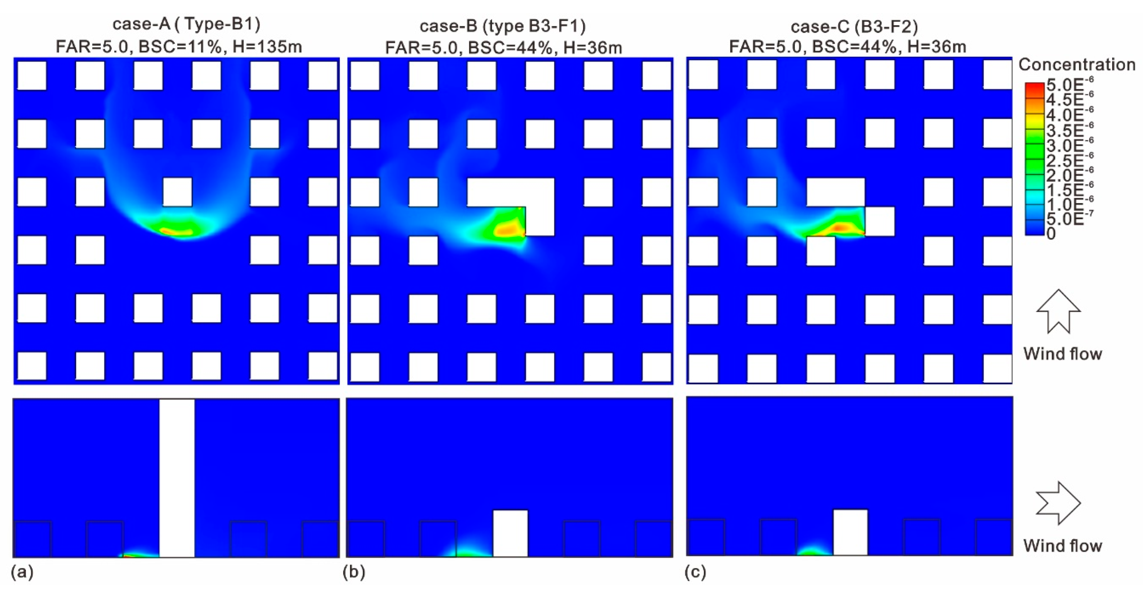
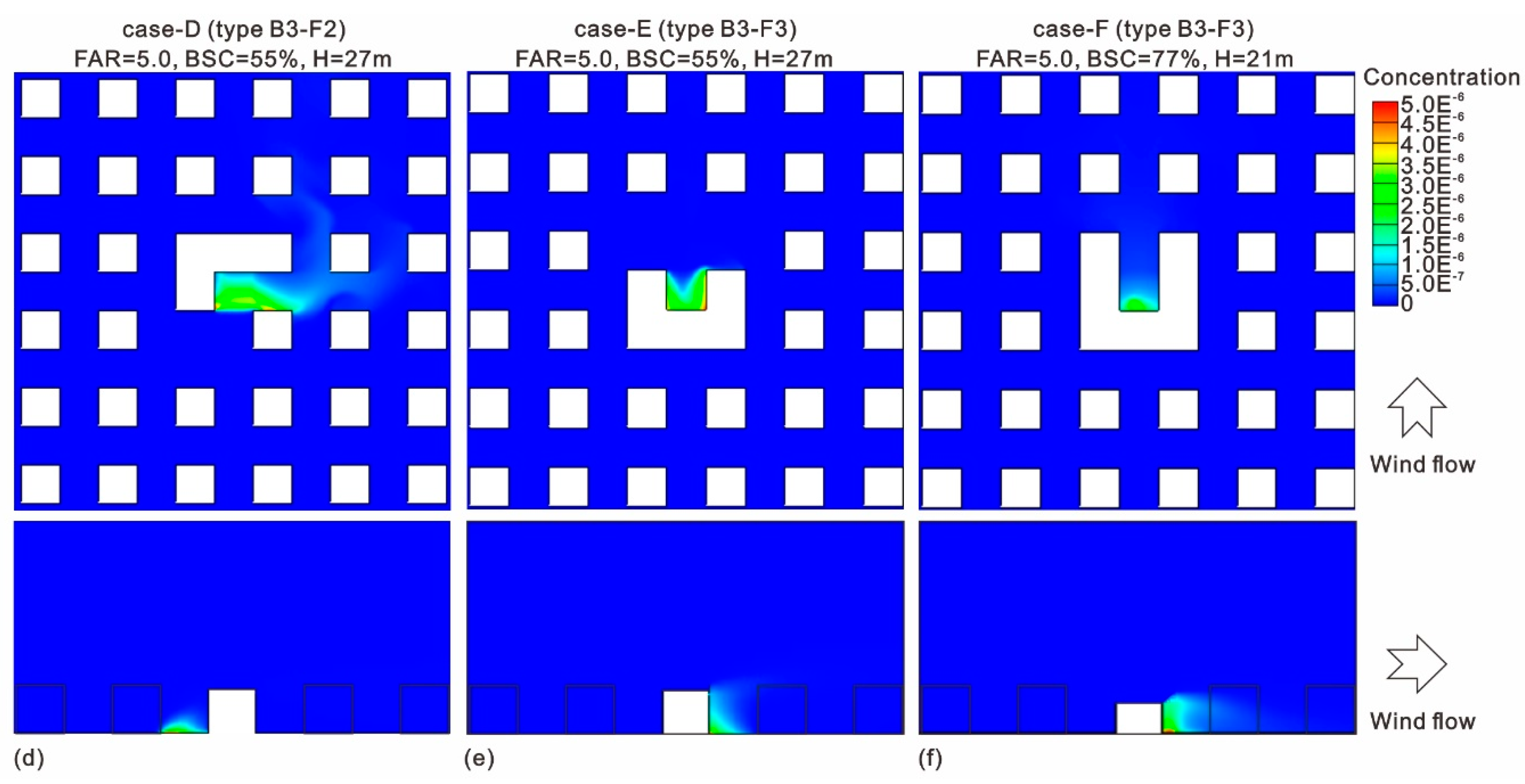
3.1. Impact of Building Layout

As an example, Figure 4 shows the wind velocity of six cases at the pedestrian level. The flow feature in Figure 4a is consistent with simulation results of previous studies [13,32,46,57], i.e., when the BSC is 11%, the flow pattern is characterized by acceleration and flow separation, reattachment flow downstream and wake region. The velocity of the central area is obviously influenced by the high-rise buildings on the leeward side. By increasing the BSC to 44%, despite that the height (H = 36 m) is much lower than that of 11% (H = 135 m), the wind flow in the central area is still blocked by the leeward buildings (Figure 4b). Further, Figure 4c,d show that, still increasing the BSC, the flow patterns are very similar, which means that although the BSC increases and the building height decreases, this configurations have a similar indirect channeling effect. Finally, Figure 4e,f show that despite the geometries are similar (with building heights of 27 m and 21 m), the flow field characteristics are obviously different, which shows that, when the current row of buildings is completely blocked, the most significant factor affecting the central area is the building height but not the long space that is enclosed by the building.
The ventilation within the plot area is obviously related to the flow patterns that are shown in Figure 4. In order to have a complete picture of the ventilation, Figure 5 shows the indices Q, PFR, NEV, and VF for the different cases investigated. The ventilation performance of C forms is always better than other types for BSC of 11% to 66%. This is expected, since such C forms are not blocked by any front leeward obstacle. In addition, when BSC is 11% (H = 135 m), the corresponding C forms are made of single independent obstacle. Although there is no obstacle blocking the wind, no channeling effect occurs, so the air flow through the central area is less than that found for BSC of 22% (H = 69 m) to 55% (H = 27 m). When BSC is 66% (H = 24 m), the corresponding C form experiences an air channeling effect, but the lower building height makes part of the airflow exchanging through the street top and thus reduces the flow through the central area. When BSC is 77% (H = 21 m), no C type is possible, but B3–F2 and B3–F3 exists. Obviously, high BSC results in less air flow flushing into the central area by mean flow. However, the lower building height induces highly vertical turbulent diffusion exchange.
Figure 5 illustrates that B3–F3 forms also experience the poorest ventilation conditions within the central area. Contrary to other types, the local ventilation performance of B3–F3 forms central area that gradually increases with increasing BSC from 33% to 77%. Overall, this suggests that when FAR is fixed and the central area is blocked by surrounding obstacles, the local ventilation efficiency can be improved by reducing the average height of the building and increasing BSC within the plot area.
It should be also noted that when BSC increases from 11% to 77% in general the ventilation efficiency within the central area decreases due to the increase of buildings within the plot area. However, looking at NEV and VF (Figure 5c,d), it can be noted that, when BSC increases from 44% to 77%, NEV and VF slightly improves. Overall, there is no clear relationship between ventilation indices and the various BSC. Therefore, in order to achieve useful conclusions on such a relationship, the average value and the error have been calculated for each configuration, and the results are discussed in the next subsection.
The ventilation performance that is analyzed in Figure 5 directly affects the concentration distribution at the pedestrian level, as shown in Figure 6. When BSC is 11%, meaning only one high-rise building (H = 135 m) in the central area, i.e., case-A (type B1), as expected from flow pattern (Figure 4), the pollutant concentration is significantly affected by the isolated high-rise building. In particular, since the central area is on the leeward side of the building, less air flows into the central area by mean flow. Due to the high level aspect ratio (H/W > 2), third or fourth recirculation occurs and weakens the capability of pollutant dilution and removal from the pedestrian level, resulting in a high concentration level in this type of configurations. When the BSC increases to 44% (H = 36 m), looking at the concentration distribution of case-B (type B3–F1) and case-C (type B3–F2), an indirect wind channeling occurs in case-C. Therefore, the mean flow passing through the central area plays a major role in removing pollutant. However, the H/W corresponding to this BSC is about 1.0. From the vertical distribution of the pollutant concentration of case-B, it can be seen that, due to the obvious obstruction, turbulent diffusion begins to influence the central pedestrian level concentration through the roof, and part of the pollutant is removed by the turbulent diffusion effect, which implies that the building height is not the main influence factor of this BSC. When the BSC increases to 55% (H = 27 m) and 77% (H = 21 m), the case-E (type B3–F3) and case-F (type B3–F3) have a relative similar H/W and architectural layout. It can be seen that the turbulence diffusion through the roof now plays a significant role in diluting the pollutant at the pedestrian level. Meanwhile, when compared with the higher level of BSC, i.e., 55%, 66%, and 77%, very few configurations with wind channeling occur. Therefore, when the BSC exceeds 55%, the BSC becomes an important factor determining the ventilation efficiency within the central area rather than the building height.

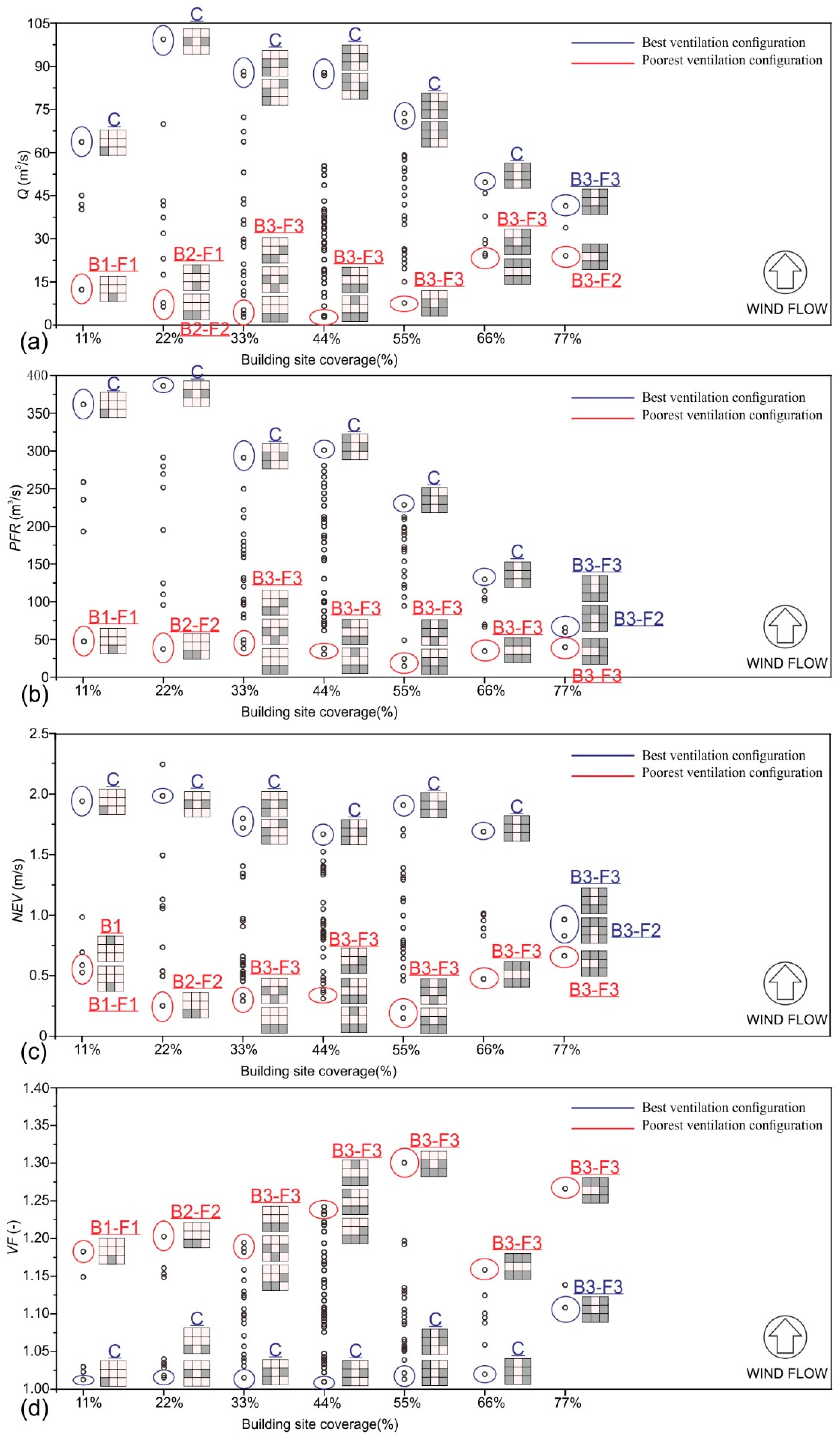
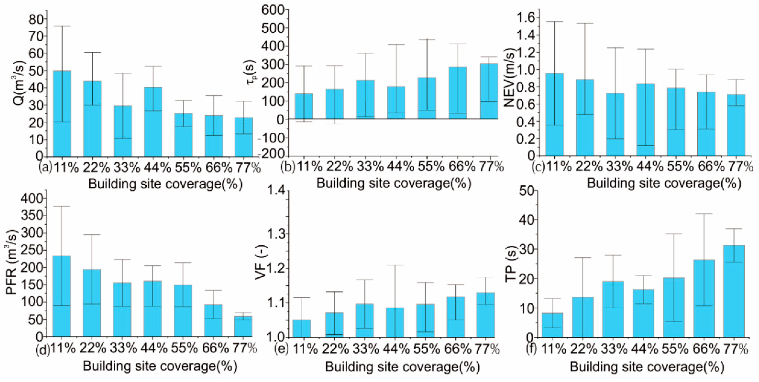
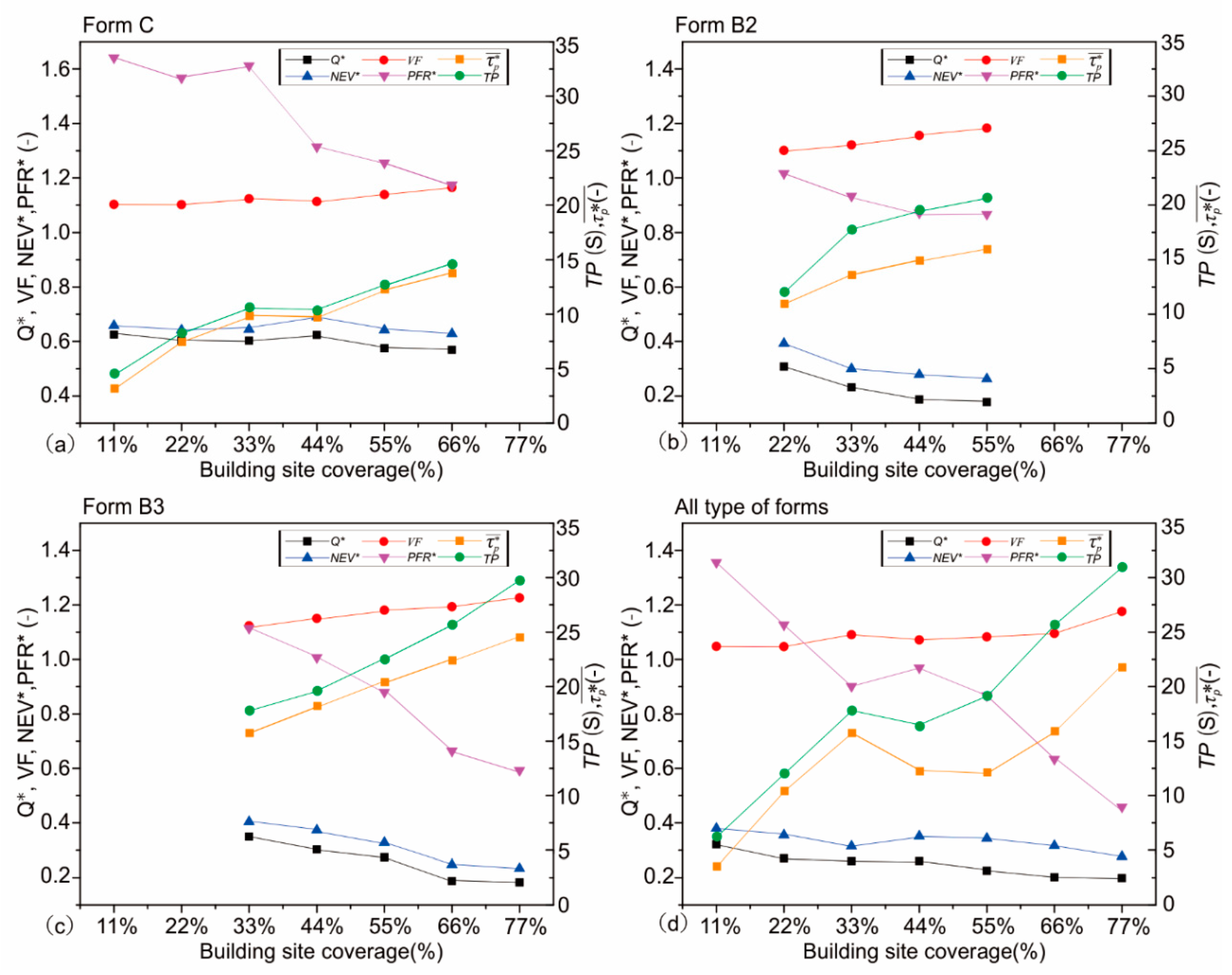
3.2. Relationship between Local Ventilation Efficiency and BSC

Figure 7 shows the average and error values of the six ventilation indices (air flow rate (Q), τp, NEV, PFR, VF, and TP) for all the configurations investigated (see Figure 2). Q, NEV, and PFR (Figure 7a,c,d) decrease gradually with increasing BSC, which indicates that the ventilation performance within the central area becomes poorer. On the other hand, τp, VF, and TP gradually rise with increasing BSC, reflecting the decrease of pollutants removal capability in the central area (Figure 7b,e,f).
It is noted that the value of the aforementioned ventilation indices stopped decreasing when the BSC becomes 44%, but there is a slight increase with increasing BSC. This is due to the large impact of C forms, while the other forms have no direct wind channeling effect due to the blockage of the buildings. As BSC continues to increase from 44% (thus the building height decreases), it can be seen that the trend of the ventilation indices is no longer obvious as happens for BSC of 11% to 44%, although the increase of BSC causes the horizontal airflow channeling to gradually decrease. In fact, due to the reduction of building height, the turbulent diffusion effect within the building roof becomes remarkable. This is consistent with the research results of [24].

3.3. Sensitivity of the Six Ventialtion Indices to the BSC

Since the purpose of this paper is to try to establish a correlation between the morphological parameters and ventilation performance parameters, it is worth evaluating how the different indices change when BSC changes (sensitivity analysis). Figure 8 shows the average normalized values of the six indices (Q*, VF, NEV*, PFR*, TP and τ p * ¯ ) of C, B2, and B3 forms.
As shown in Figure 8a (C forms), the values of each index do not change significantly with increasing BSC. This is due to the channeling effect that occurs in these cases, since, with increasing BSC, only the upwind airflow is affected and thus there is no significant effect on the air flowing in the horizontal direction downstream. For B2 forms (Figure 8b), even though BSC are lower or equal to C forms, the position change of buildings induces a significant impact on the ventilation performance within the central area. Finally, for B3 forms (Figure 8c), since the airflow is blocked upstream to the central area, the trend of each index is relatively obvious, especially for BSC of 33% to 55%. On the other hand, when BSC is 66% and 77%, the building arrangements are quite similar (i.e., there is less space to move buildings), resulting in a low change of each index.
To summarize, Figure 8d shows the trend of all the indices for all the forms (and thus for all the 101 configurations) investigated. The figure shows that PFR, τ p ¯ , and TP are the most sensitive to BSC variation up to 44%, since the wind channeling effect is expected to dominate the exchange with the underlying atmosphere. With increasing BSC (and thus the density), the wind channeling effect is not the only and effective mechanism to dilute or remove air pollutants. In fact, since the average building height is relatively low, the effect of turbulence can effectively remove the pollutants at the pedestrian level and improve the local ventilation performance. At the same time, the results have shown that BSC is not the only factor that determines the ventilation performance within the urban plot, and the building patterns within the plot area also plays a significant role on flow and pollutant dispersion.

4. Conclusions

This paper aims to investigate a quantitative correlation between urban-like geometries of different building site coverage (BSC) and six ventilation indices that are commonly employed in the literature. The floor area ratio (FAR) is kept constant at 5.0, while BSC gradually increases from 11% to 77% (while building heights H decrease from 135 m to 21 m, respectively), resulting in a total of 101 asymmetrical idealized configurations. Results show that, among the indices investigated, PFR, TP, and τ p * ¯ better correlate with urban morphological parameters. For improving ventilation and pollutant dispersion, the study has shown that:
  • when BSC is 11% (H = 135 m), 22% (H = 69 m) and 33% (H = 45 m), the density of buildings in the central area is low, and the ventilation performance is greatly affected by the large building heights, regardless of the architectural arrangement with channeling effect;
  • with increasing BSC to 44% (H = 36 m), 55% (H = 27 m), 66% (H = 24 m), and 77% (H = 21 m), the ventilation performance is slightly lower than before. However, due to the lower average building heights, more airflow flushes into the central area by turbulent flow and a vertical exchange through the roof occurs, diluting part of the pollutants; and,
  • for the same BSC, the configurations experiencing a wind channeling effect are characterized by a better ventilation.
From an urban designing and planning perspective, results suggest that, when FAR is fixed in a plot area, intermediate BSCs (and building heights) may experience airflow channels by controlling the layout, which is an effective way to increase the overall ventilation and thus the ability of pollutant dispersion. These results show that by using BSC and FAR as morphological parameters, the ventilation performance of void spaces can be effectively improved in high-density cities by reducing the average height of buildings. Specifically, a BSC = 44% (H = 36 m) of C form (i.e., no buildings in front of the central area and with channeling effect) seems to simultaneously maximize the ventilation performance and the number of possible layouts that are also available to harmonize the new built area to the existing surrounding morphology.
This study investigated idealized configurations that were subjected to a wind perpendicular to building façades and thus further research is needed when considering more complex geometries (such as, for example, secondary roads within the central area) and oblique wind directions, as well as non-isothermal conditions with strong heat fluxes and low wind events, which may be critical with respect to ventilation and human thermo-physiological conditions. Further, the impact of passive methods [58], including vegetation [59,60,61], as well as lift-up design [62], which are becoming increasingly popular in China to improve the pedestrian level wind and thermal comfort.

Supplementary Materials

The supplementary materials are available online at https://www.mdpi.com/2073-4433/10/1/33/s1.

Author Contributions

W.D. and. Z.G were responsible for the study design and supervision. Y.P. wrote the manuscript, performed the CFD simulation and conducted data analysis; R.B. revised the paper and wrote sections of the manuscript. All authors contributed to the discussion of the results and have read and approved the final manuscript.

Funding

The research was supported by the key project funded by the National Science Foundation of China on “Urban form-microclimate coupling mechanism and control”, Grant No. 51538005, and Supported by the Scientific Research Foundation of Graduate School of Nanjing University NO. 2017CL13 “Ventilation Performance and Pollutant Dispersion Mechanism under the Influence of Complex Urban Morphological Characteristics”

Conflicts of Interest

The authors declare no conflict of interest.

Nomenclature

FARfloor area ratio (%)
BSCbuilding site coverage (%)
Q flow rate (m3 s−1)
Q reference flow rate far upstream (m3 s−1)
Q * normalized flow rate through street openings or street roofs
PFRpedestrian purging flow rate
PFR*normalized pedestrian purging flow rate value
N E V p e d pedestrian net escape velocity (m/s)
VFvisitation frequency
TPpollutant residential time (s)
τ ¯ p , τ ¯ p * local mean age of air (s) and its normalized value
Scpollutant source rate (kg m−3 s−1)
Cthe spatially averaged concentration in the entire pedestrian domain (kg/m³)
Volthe pedestrian volume form ground up to 2m in the canopy (m3)
k, εturbulent kinetic energy (m2 s−2) and its dissipation rate
u A B L * atmospheric boundary layer friction velocity (m/s)
z 0 aerodynamic roughness length (m)
κthe von Karman constant
zheight coordinate (m)
Hheight of central area buildings

References

  1. Raaschounielsen, O.; Andersen, Z.J.; Beelen, R.; Samoli, E.; Stafoggia, M.; Weinmayr, G.; Hoffmann, B.; Fischer, P.; Nieuwenhuijsen, M.J.; Brunekreef, B. Air pollution and lung cancer incidence in 17 european cohorts: Prospective analyses from the european study of cohorts for air pollution effects (ESCAPE). Lancet Oncol. 2013, 14, 813–822. [Google Scholar] [CrossRef]
  2. Yoshie, R.; Mochida, A.; Tominaga, Y.; Kataoka, H.; Harimoto, K.; Nozu, T.; Shirasawa, T. Cooperative project for CFD prediction of pedestrian wind environment in the architectural institute of Japan. J. Wind. Eng. Ind. Aerodyn. 2007, 95, 1551–1578. [Google Scholar] [CrossRef]
  3. Ketzel, M.; Berkowicz, R.; Lohmeyer, A. Comparison of numerical street dispersion models with results from wind tunnel and field measurements. Environ. Monit. Assess. 2000, 65, 363–370. [Google Scholar] [CrossRef]
  4. Blocken, B.; Stathopoulos, T.; Carmeliet, J.; Hensen, J.L.M. Application of computational fluid dynamics in building performance simulation for the outdoor environment: An overview. J. Build. Perform. Simul. 2011, 4, 157–184. [Google Scholar] [CrossRef]
  5. Franke, J.; Hellsten, A.; Schlünzen, H.; Carissimo, B. Best Practice Guideline for the Cfd Simulation of Flows in the Urban Environment; COST Office: Brussels, Belgium, 2007. [Google Scholar]
  6. Tominaga, Y.; Mochida, A.; Yoshie, R.; Kataoka, H.; Nozu, T.; Yoshikawa, M.; Shirasawa, T. Aij guidelines for practical applications of cfd to pedestrian wind environment around buildings. J. Wind. Eng. Ind. Aerodyn. 2008, 96, 1749–1761. [Google Scholar] [CrossRef]
  7. Blocken, B. Computational fluid dynamics for urban physics: Importance, scales, possibilities, limitations and ten tips and tricks towards accurate and reliable simulations. Build. Environ. 2015, 91, 219–245. [Google Scholar] [CrossRef]
  8. Tominaga, Y.; Stathopoulos, T. Ten questions concerning modeling of near-field pollutant dispersion in the built environment. Build. Environ. 2016, 105, 390–402. [Google Scholar] [CrossRef]
  9. Etheridge, D.W.; Sandberg, M. Building Ventilation. Theory and Measurement; John Wiley & Sons: Chichester, NY, USA, 1996. [Google Scholar]
  10. Sandberg, M.; Sjöberg, M. The use of moments for assessing air quality in ventilated rooms. Build. Environ. 1983, 18, 181–197. [Google Scholar] [CrossRef]
  11. Awbi, H.B. Ventilation of Buildings; E & FN Spon: London, UK, 1991. [Google Scholar]
  12. Chen, Q. Ventilation performance prediction for buildings: A method overview and recent applications. Build. Environ. 2009, 44, 848–858. [Google Scholar] [CrossRef]
  13. Bady, M.; Kato, S.; Huang, H. Towards the application of indoor ventilation efficiency indices to evaluate the air quality of urban areas. Build. Environ. 2008, 43, 1991–2004. [Google Scholar] [CrossRef]
  14. Kato, S.; Huang, H. Ventilation efficiency of void space surrounded by buildings with wind blowing over built-up urban area. J. Wind. Eng. Ind. Aerodyn. 2009, 97, 358–367. [Google Scholar] [CrossRef]
  15. Hang, J.; Sandberg, M.; Li, Y. Age of air and air exchange efficiency in idealized city models. Build. Environ. 2009, 44, 1714–1723. [Google Scholar] [CrossRef]
  16. Buccolieri, R.; Sandberg, M.; Di Sabatino, S. City breathability and its link to pollutant concentration distribution within urban-like geometries. Atmos. Environ. 2010, 44, 1894–1903. [Google Scholar] [CrossRef]
  17. Hang, J.; Li, Y.; Sandberg, M.; Buccolieri, R.; Di Sabatino, S. The influence of building height variability on pollutant dispersion and pedestrian ventilation in idealized high-rise urban areas. Build. Environ. 2012, 56, 346–360. [Google Scholar] [CrossRef]
  18. Kato, S.; Ito, K.; Murakami, S. Analysis of visitation frequency through particle tracking method based on les and model experiment. Indoor Air 2010, 13, 182–193. [Google Scholar] [CrossRef]
  19. Neophytou, M.; Britter, R. Modelling of atmospheric dispersion in complex urban topographies: A computational fluid dynamics study of the central London area. In Proceedings of the 5th GRACM International Congress on Computational Mechanics, Limassol, Cyprus, 29 June–1 July 2005. [Google Scholar]
  20. Panagiotou, I.; Neophytou, K.A.; Hamlyn, D.; Britter, R.E. City breathability as quantified by the exchange velocity and its spatial variation in real inhomogeneous urban geometries: An example from central london urban area. Sci. Total. Environ. 2013, 442, 466–477. [Google Scholar] [CrossRef] [PubMed]
  21. Liu, C.H.; Leung, D.Y.C.; Barth, M.C. On the prediction of air and pollutant exchange rates in street canyons of different aspect ratios using large-eddy simulation. Atmos. Environ. 2005, 39, 1567–1574. [Google Scholar] [CrossRef]
  22. Kubilay, A.; Neophytou, K.A.; Matsentides, S.; Loizou, M.; Carmeliet, J. The pollutant removal capacity of an urban street canyon and its link to the breathability and exchange velocity. Procedia Eng. 2017, 180, 443–451. [Google Scholar] [CrossRef]
  23. Lim, E.; Ito, K.; Sandberg, M. New ventilation index for evaluating imperfect mixing conditions—Analysis of net escape velocity based on rans approach. Build. Environ. 2013, 61, 45–56. [Google Scholar] [CrossRef]
  24. Hang, J.; Wang, Q.; Chen, X.; Sandberg, M.; Zhu, W.; Buccolieri, R.; Di Sabatino, S. City breathability in medium density urban-like geometries evaluated through the pollutant transport rate and the net escape velocity. Build. Environ. 2015, 94, 166–182. [Google Scholar] [CrossRef]
  25. Lim, E.; Ito, K.; Sandberg, M. Performance evaluation of contaminant removal and air quality control for local ventilation systems using the ventilation index net escape velocity. Build. Environ. 2014, 79, 78–89. [Google Scholar] [CrossRef]
  26. Antoniou, N.; Montazeri, H.; Wigo, H.; Neophytou, M.; Blocken, B.; Sandberg, M. CFD and wind-tunnel analysis of outdoor ventilation in a real compact heterogeneous urban area: Evaluation using “air delay”. Build. Environ. 2017, 126, 355–372. [Google Scholar] [CrossRef]
  27. Hang, J.; Li, Y.; Sandberg, M.; Claesson, L. Wind conditions and ventilation in high-rise long street models. Build. Environ. 2010, 45, 1353–1365. [Google Scholar] [CrossRef] [Green Version]
  28. Oke, T.R. Street design and urban canopy layer climate. Energy Build. 1988, 11, 103–113. [Google Scholar] [CrossRef]
  29. Sini, J.F.; Anquetin, S.; Mestayer, P.G. Pollutant dispersion and thermal effects in urban street canyons. Atmospheric Environ. 1996, 30, 2659–2677. [Google Scholar] [CrossRef]
  30. Salim, S.M.; Buccolieri, R.; Chan, A.; Di Sabatino, S. Numerical simulation of atmospheric pollutant dispersion in an urban street canyon: Comparison between rans and les. J. Wind Eng. Ind. Aerodyn. 2011, 99, 103–113. [Google Scholar] [CrossRef]
  31. Thaker, P.; Gokhale, S. The impact of traffic-flow patterns on air quality in urban street canyons. Environ. Pollut. 2016, 208, 161–169. [Google Scholar] [CrossRef]
  32. Ramponi, R.; Blocken, B.; Coo, L.B.D.; Janssen, W.D. CFD simulation of outdoor ventilation of generic urban configurations with different urban densities and equal and unequal street widths. Build. Environ. 2015, 92, 152–166. [Google Scholar] [CrossRef] [Green Version]
  33. Yuan, C.; Ng, E.; Norford, L.K. Improving air quality in high-density cities by understanding the relationship between air pollutant dispersion and urban morphologies. Build. Environ. 2014, 71, 245–258. [Google Scholar] [CrossRef]
  34. Peng, Y.; Gao, Z.; Ding, W. An approach on the correlation between urban morphological parameters and ventilation performance. Energy Procedia 2017, 142, 2884–2891. [Google Scholar] [CrossRef]
  35. Kubota, T.; Miura, M.; Tominaga, Y.; Mochida, A. Wind tunnel tests on the relationship between building density and pedestrian-level wind velocity: Development of guidelines for realizing acceptable wind environment in residential neighborhoods. Build. Environ. 2008, 43, 1699–1708. [Google Scholar] [CrossRef]
  36. Hang, J.; Sandberg, M.; Li, Y. Effect of urban morphology on wind condition in idealized city models. Atmos. Environ. 2009, 43, 869–878. [Google Scholar] [CrossRef]
  37. Yoshie, R.; Tanaka, H.; Shirasawa, T.; Kobayashi, T. Experimental study on air ventilation in a built-up area with closely-packed high-rise buildings. J. Environ. Eng. 2008, 73, 661–667. [Google Scholar] [CrossRef]
  38. Buccolieri, R.; Salizzoni, P.; Soulhac, L.; Garbero, V.; Di Sabatino, S. The breathability of compact cities. Urban Clim. 2015, 13, 73–93. [Google Scholar] [CrossRef]
  39. Hang, J.; Li, Y.; Buccolieri, R.; Sandberg, M.; Di Sabatino, S. On the contribution of mean flow and turbulence to city breathability: The case of long streets with tall buildings. Sci. Total. Environ. 2012, 416, 362–373. [Google Scholar] [CrossRef]
  40. Hu, T.; Yoshie, R. Indices to evaluate ventilation efficiency in newly-built urban area at pedestrian level. J. Wind Eng. Ind. Aerodyn. 2013, 112, 39–51. [Google Scholar] [CrossRef]
  41. Shen, J.; Gao, Z.; Ding, W.; Yu, Y. An investigation on the effect of street morphology to ambient air quality using six real-world cases. Atmos. Environ. 2017, 164, 85–101. [Google Scholar] [CrossRef]
  42. Yazid, A.W.M.; Sidik, N.A.C.; Salim, S.M.; Saqr, K.M. A review on the flow structure and pollutant dispersion in urban street canyons for urban planning strategies. Simulation 2014, 90, 892–916. [Google Scholar] [CrossRef]
  43. Di Sabatino, S.; Buccolieri, R.; Kumar, P. Spatial distribution of air pollutants in cities. In Clinical Handbook of Air Pollution-Related Diseases; Springer: Berlin, Germany, 2018; pp. 75–95. [Google Scholar]
  44. Buccolieri, R.; Wigö, H.; Sandberg, M.; Di Sabatino, S. Direct measurements of the drag force over aligned arrays of cubes exposed to boundary-layer flows. Environ. Fluid Mech. 2017, 17, 1–22. [Google Scholar] [CrossRef]
  45. Tominaga, Y. Visualization of city breathability based on cfd technique: Case study for urban blocks in niigata city. J. Vis. 2012, 15, 269–276. [Google Scholar] [CrossRef]
  46. Mittal, H.; Sharma, A.; Gairola, A. A review on the study of urban wind at the pedestrian level around buildings. J. Build. Eng. 2018, 18, 154–163. [Google Scholar] [CrossRef]
  47. Tominaga, Y.; Stathopoulos, T. Numerical simulation of dispersion around an isolated cubic building: Model evaluation of rans and les. Build. Environ. 2010, 45, 2231–2239. [Google Scholar] [CrossRef]
  48. Liu, J.; Niu, J. Cfd simulation of the wind environment around an isolated high-rise building: An evaluation of srans, les and des models. Build. Environ. 2016, 96, 91–106. [Google Scholar] [CrossRef]
  49. Tominaga, Y.; Mochida, A.; Murakami, S.; Sawaki, S. Comparison of various revised k-ε models and les applied to flow around a high-rise building model with 1:1:2 shape placed within the surface boundary layer. J. Wind Eng. Ind. Aerodyn. 2008, 96, 389–411. [Google Scholar] [CrossRef]
  50. Moonen, P.; Dorer, V.; Carmeliet, J. Evaluation of the Ventilation Potential of Countyards and Urban Street Canyons Using RANS and LES. J. Wind. Eng. Ind. 2011, 99, 414–423. [Google Scholar] [CrossRef]
  51. Gousseau, P.; Blocken, B.; Stathopoulos, T.; van Heijst, G.J.F. CFD simulation of near-field pollutant dispersion on a high-resolution grid: A case study by les and rans for a building group in downtown montreal. Atmos. Environ. 2011, 45, 428–438. [Google Scholar] [CrossRef]
  52. Blocken, B.I. 50 years of computational wind engineering: Past, present and future. J. Wind. Eng. Ind. Aerodyn. 2014, 129, 69–102. [Google Scholar] [CrossRef]
  53. Blocken, B. LES over RANS in building simulation for outdoor and indoor applications: A foregone conclusion? Build. Simul. 2018, 11, 821–870. [Google Scholar] [CrossRef]
  54. Richards, P.; Hoxey, R. Appropriate boundary conditions for computational wind engineering model using the k-ε turbulence model. In Computational Wind Engineering 1; Elsevier: Amsterdam, The Netherlands, 1993; pp. 145–153. [Google Scholar]
  55. Yao, Y. Nanjing: Historical Landscape and Its Planning from Geographical Perspective; Springer Geography: Berlin, Germany, 2016; p. 221. [Google Scholar]
  56. Hang, J.; Li, Y. Age of air and air exchange efficiency in high-rise urban areas and its link to pollutant dilution. Atmos. Environ. 2011, 45, 5572–5585. [Google Scholar] [CrossRef]
  57. Princevac, M.; Baik, J.J.; Li, X.; Pan, H.; Park, S.B. Lateral channeling within rectangular arrays of cubical obstacles. J. Wind. Eng. Ind. Aerodyn. 2010, 98, 377–385. [Google Scholar] [CrossRef]
  58. Gallagher, J.; Baldauf, R.; Fuller, C.H.; Kumar, P.; Gill, L.W.; McNabola, A. Passive methods for improving air quality in the built environment: A review of porous and solid barriers. Atmos. Environ. 2015, 120, 61–70. [Google Scholar] [CrossRef]
  59. Buccolieri, R.; Santiago, J.L.; Rivas, E.; Sánchez, B. Review on urban tree modelling in cfd simulations: Aerodynamic, deposition and thermal effects. Urban For. Urban Green. 2018, 31, 212–220. [Google Scholar] [CrossRef]
  60. Santamouris, M.; Ban-Weiss, G.; Osmond, P.; Paolini, R.; Synnefa, A.; Cartalis, C.; Muscio, A.; Zinzi, M.; Morakinyo, T.E.; Ng, E.; et al. Progress in urban greenery mitigation science–assessment methodologies advanced technologies and impact on cities. J. Civ. Eng. 2018, 24, 638–671. [Google Scholar] [CrossRef]
  61. Tan, Z.; Lau, K.L.; Ng, E. Urban tree design approaches for mitigating daytime urban heat island effects in a high-density urban environment. Energy Build. 2016, 114, 265–274. [Google Scholar] [CrossRef]
  62. Du, Y.; Mak, C.M.; Li, Y. Application of a multi-variable optimization method to determine lift-up design for optimum wind comfort. Build. Environ. 2018, 131, 242–254. [Google Scholar] [CrossRef]
Figure 1. Description of floor area ratio (FAR) and building site coverage (BSC). The yellow area is the plot area considered in this paper (which can be covered by buildings), while the blue area is the central area which cannot be covered by buildings and where the ventilation indices are calculated.
Atmosphere 10 00033 g001
Figure 2. Idealized configurations with BSC increasing from 11% to 77% in the plot area, with indication of building heights and forms. Please note that the wind blows from below.
Atmosphere 10 00033 g002
Figure 3. Schematic sketch of the computational domain and boundary conditions used in Computational Fluid Dynamics (CFD) simulations. The yellow area represents the plot area (see Figure 1).
Atmosphere 10 00033 g003
Figure 4. Velocity magnitude at pedestrian level for BSC equal to (a) 11%, (b,c) 44%, (d,e) 55%, (f) 77%.
Atmosphere 10 00033 g004
Figure 5. Values of ventilation indices (a) air flow rate (Q), (b) purging flow rate (PFR), (c) net escape velocity (NEV), and (d) visitation frequency (VF) for each configuration with BSC increasing from 11% to 77%. The best (blue) and poorest (red) configurations and the corresponding forms are explicitly indicated.
Atmosphere 10 00033 g005
Figure 6. Pollutant concentration at pedestrian level and vertical distribution for BSC equal to (a) 11%, (b,c) 44%, (d,e) 55%, and (f) 77%.
Atmosphere 10 00033 g006aAtmosphere 10 00033 g006b
Figure 7. Average values and variances of ventilation indices (a) Q, (b) τp, (c) NEV, (d) PFR, (e) VF, and, (f) resident time (TP) for all the configurations with BSC increasing from 11% to 77%.
Atmosphere 10 00033 g007
Figure 8. Average values of the six ventilation for all of the configurations with BSC increasing from 11% to 77%: (a) C forms, (b) B2 forms, (c) B3 forms, and (d) all type of forms.
Atmosphere 10 00033 g008
Table 1. CFD simulation condition settings.
Calculation conditionsSolver settings
Computational domain(x)1080 m × (y)1920 m × (z)525 m
Grid resolutionabout 2 million hexahedral cells
Turbulence modelStandard k–ε turbulence model
Algorithm for pressure-velocitySIMPLE
Scheme for advection termsSecond-order discretization for convection terms and the viscous terms
Boundary conditionsInflow: Boundary condition presented by Richards and Hoxey (1993)
Outflow: Zero gradient condition
Ground and block surfaces: Non-slip wall
Top and lateral surfaces: Symmetry

