On the Roles of Advection and Solar Heating in Seasonal Variation of the Migrating Diurnal Tide in the Stratosphere, Mesosphere, and Lower Thermosphere

Abstract

The migrating diurnal tide (DW1) presents a unique latitudinal structure in the stratosphere, mesosphere, and lower thermosphere. In this paper, the physical mechanisms that govern its seasonal variation are examined in these three regions using the 31.5-year (1979–2010) output from the extended Canadian Middle Atmosphere Model (eCMAM30). DW1 annual variation in the stratosphere is mainly controlled by the short-wave heating in the high latitudes, but by both the short-wave and adiabatic heating in the low latitudes. In the mesosphere, linear and nonlinear advection play important roles in the semiannual variation of the tide whereas short-wave heating does not. In the lower thermosphere, the annual variation of DW1 is mainly governed by the short-wave heating and linear advection. This study illustrates the complexity of the main physical mechanisms modulating the seasonal variations of DW1 in different regions of the atmosphere.

1. Introduction

Atmospheric thermal tides are dominant global-scale wave motions in the middle and upper atmosphere. They can be excited by the absorption of solar radiation from tropospheric water vapor (H₂O) and stratospheric ozone (O₃) [1,2,3], latent heat release of deep convective systems [4,5], as well as nonlinear interactions between tides and planetary waves (PWs) [6,7,8]. Atmospheric tides can also be generated in-situ by the absorption of far ultraviolet (FUV) and extreme ultraviolet (EUV) radiation in the thermosphere by atomic oxygen (O), molecular oxygen (O₂), and molecular nitrogen (N₂) [3,9,10]. Atmospheric tides can significantly influence the thermal and dynamical structure of the atmosphere through their interaction with the mean flow and other waves [6,11,12,13,14]. Tides generated in the lower atmosphere can propagate upwards and deposit their energy and momentum in the upper atmosphere through dissipation processes and induce profound effects on the ionosphere and thermosphere [15,16,17,18].

The migrating diurnal tide (named as DW1: D is for diurnal—24 h period, W is for westward propagation, and 1 is zonal wavenumber) is one of the largest atmospheric tides at the low latitudes of 50–120 km above the Earth’s surface [3,19,20]. Its amplitude exhibits a strong semiannual variation with maxima during equinox and minima during solstice, which was first identified by the Upper Atmosphere Research Satellite (UARS) wind measurements [21].

In addition, DW1 is known to present different latitudinal structure and seasonal variation (e.g., annual variation with maximum in summer hemisphere) in the stratosphere [22,23]. There have been very few studies conducted to explain the seasonal variation in this region [24]. DW1 can also be generated in-situ by the EUV-radiation in the lower thermosphere (>120 km) and present a different latitudinal structure from that in the mesosphere [25]. Global satellite-borne observations of the neutral dynamics between 120 and 400 km are currently nonexistent (termed the ‘thermospheric gap’ [26]). Oberheide et al. (2011) [26] tried to use the Climatological Tidal Model of the Thermosphere (CTMT) to fill this gap. The CTMT uses tidal observations in the mesosphere and extends them into the thermosphere using the Hough Model Extension (HME), but no in-situ DW1 excited by the solar EUV radiation is included in the model. Forbes et al. (2011) [27] diagnosed in-situ DW1 from the CHAMP (Challenging Minisatellite Payload) and GRACE (Gravity Recovery and Climate Experiment) data in the upper thermosphere at 400 km. Few modeling studies have been conducted to study the DW1 features in the thermosphere above 120 km [9,28,29].

Possible physical mechanisms proposed to explain the observed seasonal variation of DW1 include variation in the heating sources that force the tide, propagation modulation due to altered background mean wind, and the nonlinear interaction with planetary waves and/or gravity waves [19,20,30]. Previous studies have mainly focused on the explanation of DW1 seasonal variation in this region although the dominant physical processes still remain debatable [19,20,31,32,33,34]. Tidal momentum and thermodynamic budget analyses [19,35,36] have been used to establish direct cause and effect of DW1 in the mesosphere. Using a 2-year climatology simulation from an older version of the eCMAM, McLandress (2002a) [19] conducted the budget analyses of DW1 and found that the linear advection term (DW1—mean flow interaction) plays an important role in the seasonal variation of the tide. Following the same methodology and using the Whole Atmosphere Community Climate Model, version 4 (WACCM4), Lu et al. (2012) [36] concluded that both gravity wave (GW) forcing and the linear advection are important in determining the zonal wind structure of DW1 in March. Based on 8 years (2002–2009) of measurements from the Thermosphere- Ionosphere-Mesosphere Energetic and Dynamics (TIMED) satellite, Lieberman et al. (2010) [35] diagnosed the leading terms of the momentum budget of DW1 and found that besides the classical terms (e.g., the Coriolis and pressure gradient forces), the meridional advection of the zonally averaged momentum and wave drag effects are also important.

In this paper, we expand the thermodynamic budget analyses on DW1 as in McLandress (2002a) [19] to include the stratosphere and lower thermosphere (up to ~200 km). To our knowledge, no such studies have been conducted to investigate the physical mechanisms of the seasonal variation of DW1 in these two atmospheric layers. Such study is also necessary in the mesosphere because of model updates. The new version of the model includes interactive chemistry, simplified ion chemistry, realistic sea surface temperature and solar cycle. The lower part of the model is also nudged to reanalysis data and thus includes realistic quasi-biannual oscillation (QBO) in the stratosphere. The results presented in this study are based on a 31.5-year climatological mean (Jan 1979–June 2010). McLandress (2002a) [19] only illustrated results at two latitudes (20° N and 20° S) in two months (April and July) using one-year data. Full latitude range between 85° S and 85° N and all twelve months are studied in this paper.

The objective of this paper is to examine the role of advection (including linear and nonlinear) and solar heating in governing the seasonal variations of DW1 in the stratosphere, mesosphere, and lower thermosphere. Linear advection describes wave-mean flow interaction while nonlinear advection represents wave-wave interaction. We emphasize on the similarity, difference, and complexity of the above mechanisms in the three atmospheric layers. The nudged model run’s capability in reproducing the altitude–latitude structures and seasonal variations of DW1 between 20 and 110 km has been evaluated by Gan et al. (2014) [37] with the Sounding of the Atmosphere using Broadband Emission Radiometry (SABER) observations. The latitude-altitude structure and seasonal variation of DW1 in the lower thermosphere (130 to 220 km) from the eCMAM30 compares well with the Thermosphere Ionosphere Electrodynamic General Circulation model (TIE-GCM) [28,29], the thermospheric extension of the global-scale wave model (GSWM) [38] and the thermospheric extension of the Whole Atmosphere Community Climate Model (WACCM-X) [39]. However, the tidal amplitudes in this region show large discrepancy among the models. The Sun-synchronous Michelson Interferometer for Passive Atmospheric Sounding (MIPAS) can provide superposition of tidal components with odd frequency up to 150 km, but does not allow the separation of individual tidal components [40]. Although a full characterization of the thermosphere wave spectrum has to await future dedicated satellite missions; e.g., Global-scale observations of the Limb and Disk (GOLD, launched on 25 Jan 2018) and Ionospheric Connection Explorer (ICON, to be launched on 7 Nov 2018)—it is nevertheless useful to analyze the tidal fields in this region from self-consistent GCMs to investigate their physical mechanisms. If disagreements are found with the new satellite data in the near future, the results here will shed some light on the part(s) of the model physics that is (are) needed for improvement.

This paper is arranged as follows. Section 2 gives a brief introduction of the model, a detailed description on the data and analysis method. The altitude and latitude structures of DW1 T in the stratosphere, mesosphere, and lower thermosphere (up to ~200 km) are presented as our motivation for this study. Section 3 presents the seasonal variations of the tide and its thermodynamic budget analysis from 31.5-year climatological mean in three atmospheric layers. We will mainly focus on the two mechanisms: advection and solar heating, and with their relative roles discussed. Section 4 is the conclusions.

2. Model, Data and Method

2.1. Model

The eCMAM is a full GCM extending from the Earth’s surface to ~220 km, depending on the solar cycle [41,42]. The model is a global spectral model and has a triangular spectral truncation of T32, corresponding to a 6° × 6° latitudinal–longitudinal resolution. There are 87 levels in the vertical, with different resolutions from several tens of meters in the lower troposphere to approximately 2.5 km in the mesosphere and lower thermosphere (MLT) region. The eCMAM is developed from the standard CMAM by extending the upper boundary from 95 km to about 220 km, providing a dissipation region for upward propagating waves via molecular diffusion and ion drag [42]. Apart from the physical parameterizations inherited from the standard CMAM, new physical parameterizations are added to reflect the physical processes in the MLT region [42,43]. These physical parameterizations mainly include: modified non-orographic gravity wave drag [44,45], molecular heat diffusion and viscosity, extreme ultraviolet radiation, chemical heating, and ion drag. The extended model has been demonstrated to generate the tidal oscillations reasonably well under the free-running mode [46,47,48].

The new version of the model has a comprehensive interactive neutral chemistry applied above 400 mb [49] and a simplified interactive ion chemistry scheme [50,51] applied above approximately 80 km. These chemistry schemes altogether include 49 neutral species, electrons, and 5 ions and employ 102 neutral, 27 ion and 49 photolysis reactions. Approximately 99% of the neutral atmosphere is actively simulated, the remaining 1% being noble gases.

Recently, the horizontal winds and temperature from eCMAM are nudged (i.e., relaxed) to the 6-h horizontal winds and temperature from the European Center for Medium-Range Weather Forecasts (ECMWF) Interim Re-Analysis (ERA-Interim) [52] below 10 hPa from January 1979 to June 2010 (hence eCMAM30). Between 10 hPa and 1 hPa the amount of nudging is linearly reduced to zero, so that above 1 hPa the model is free running. The nudging approach is designated primarily to constrain synoptic space and times scales in the model, which are well represented in the reanalysis data. More details about this nudging approach can be found in McLandress (2013) [53]. No nudging of chemistry fields is included in eCMAM30.

The sea surface temperature (SST) in the eCMAM30 is slaved to monthly global-complete fields of SST and sea ice concentration at each latitude-longitude grid from the Met Office Hadley Center’s sea ice and sea surface temperature data set (HadISST) during the same time period of 1979–2010. The solar irradiance scheme in the model takes into account the day-to-day variations of the spectral solar irradiance (SSI) over the full solar cycle [54,55]. The spectral solar irradiance is specified using the data from SOLARIS-HEPPA (2011) website and the F_10.7cm index is taken from the international Reference Ionosphere (IRI) 2007 model package [51]. Medium geomagatic forcing is set as a constant in the ion drag scheme. The nudged eCMAM30 is capable of realistically reproducing the climatology of the background temperature and diurnal tidal components when compared to SABER observations [37].

We extract the global horizontal winds (u, v), temperatures (T), and parameterized model physics forcing terms from eCMAM30 every 6 h. To obtain the amplitudes and phases of DW1 in the above fields, a 2-D Fourier transform in longitude and time is applied to get the spectrum density in the domain of wave frequency and zonal wave number. On the basis of the spectrum density corresponding to DW1, an inverse Fourier transform is then used to derive its amplitude and phase. Monthly climatological mean amplitude and phase of DW1 are calculated by vector averaging between January 1979 and June 2010.

2.2. Thermodynamic Budget Equations

Equation (1) describes the thermodynamic budget of the atmosphere,

$$\frac{\partial T}{\partial t}=-\overrightarrow{V}\cdot \nabla T-\frac{\omega RT}{C_{p}P}+Q_{short}+Q_{long}+Q_{chemical}+Q_{convective}+Q_{diff}+Q_{other}$$

(1)

The advection term in Equation (1) can be expanded as:

$$F_{advert,T}=-\overrightarrow{V}\cdot \nabla T=-(\frac{u}{a\cos \theta }\frac{\partial T}{\partial \lambda }+\frac{v}{a}\frac{\partial T}{\partial \theta }+\omega \frac{\partial T}{\partial z})$$

(2)

In the above two equations u, v, T are zonal wind, meridional wind, and temperature respectively. The mean radius of Earth is designated by a and ω is vertical velocity in Pa/s. θ and λ are latitude and longitude, respectively. R is dry air gas constant and C_p is the specific heat at constant pressure.

The left-hand-side (LHS) of Equation (1) is temperature tendency (heating rate). Thermodynamic budget terms on the right-hand-side (RHS) are divided into three categories: advection (first term), adiabatic heating (second term) and total diabatic heating (the remaining six terms). Q_short and Q_long are the short-wave heating and long-wave cooling, respectively; Q_chemical is chemical heating and Q_convective is the heating due to convective adjustment; Q_diff is the heating due to vertical diffusion, and Q_other is all other terms and includes such processes as eddy vertical diffusion, GW heating, conversion of kinetic energy into heat resulting from the dissipation of horizontal winds and the effect of nudging [41]. We have checked the sum of the RHS except Q_other, and found it resembles the LHS in all three atmosphere regions. Q_other can be obtained from the difference between the LHS and RHS terms. It is generally within 10% of the total budget (figures not shown). In this paper, we will focus on Q_short and advection terms. 2D FFT is applied to temperature output to obtain the DW1 amplitude and phase. Tidal oscillations in temperature are defined as

$$T^{\prime }=\widehat{T}{e}^{-i\left(wt+s\lambda \right)}=A{e}^{ip}{e}^{-i\left(wt+s\lambda \right)}$$

where $\widehat{T}$ is complex amplitude of temperature where $\widehat{T}$ = Ae^ip, A is tidal amplitude and p is tidal phase, s is zonal wave number (s = 1 for DW1). The absolute value of the LHS can be written as

$$LHS=\left|\frac{\partial T^{\prime }}{\partial t}\right|=w\cdot A$$

where w is tidal frequency (w = 2π for DW1). The LHS of Equation (1) becomes tidal amplitude in temperature multiply a constant 2π for DW1. We calculate the terms on the RHS of Equation (1) such as advection and adiabatic terms directly using the wind and temperature outputs from the model. The parameterized heating terms are direct output from the model. We then perform 2D FFT on the RHS terms to obtain the DW1 components for each forcing terms. By analyzing the various terms on the RHS of the equation, we should gain some insights into the causes of the tidal amplitude variations on the LHS.

We can further separate the advection term into linear advection term (wave-mean interaction) and nonlinear advection term (wave-wave interaction). Substituting the linearization expressions, and, into Equation (2) and similar to that in Lu et al. (2012) [36], the linear advection term can be written as follows:

$$F_{linearadvect,T}=-\frac{\overline{u}}{a\cos \theta }\frac{\partial T^{\prime }}{\partial \lambda }-\frac{\overline{v}}{a}\frac{\partial T^{\prime }}{\partial \theta }-\frac{v^{\prime }}{a}\frac{\partial \overline{T}}{\partial \theta }-\overline{w}\frac{\partial T^{\prime }}{\partial z}-w^{\prime }\frac{\partial \overline{T}}{\partial z}$$

(3)

The complex amplitude of the nonlinear advection term can then be obtained by subtracting the complex amplitude of the linear advection term from the complex amplitude of the total advection term. The nonlinear advection term includes all the large-scale waves in the model including resolved gravity waves.

When different terms are combined, complex amplitudes are used so both amplitude and phase are taken into account. The RHS is the sum of the complex amplitudes of all terms on the RHS of the equations except Q_other. The full advection term is the sum of the complex amplitudes of nonlinear and linear advection terms. Only absolute value of the complex amplitude is shown in the paper.

2.3. Three Latitudinal Structures of DW1 in Three Regions

DW1 is known to have different latitude–altitude structures in the vertical domain of the atmosphere [23,24]. Figure 1 shows the latitude–height cross-sections of DW1 amplitudes for temperature T in March: stratosphere (10–50 km), mesosphere (50–100 km) and lower thermosphere (100–200 km). The amplitudes show four distinct latitudinal structures with height. DW1 T amplitude (<0.5 K) maximizes over the equator in the stratosphere below 35 km. The latitudinal structure changes above 35 km. DW1 T maximizes in the middle latitudes (30°–50°) of both hemispheres with a secondary maximum in the tropics. The maxima are generally symmetric about the equator although slightly stronger amplitude is observed in the SH than its NH counterpart. The latitude-altitude structures of DW1 T in the stratosphere compare very well with the Modern Era Retrospective analysis for Research and Applications (MERRA) data shown in Sakazaki et al. (2012) [24]. Derived from the classical tidal theory [56], heating in the lower atmosphere excites both propagating and trapped Hough modes. Hough modes with negative equivalent depths, and corresponding imaginary vertical wavenumbers, have latitudinal structure functions that maximize in middle and high latitudes. When these modes are forced, they cannot propagate upwards and the response is trapped to the region of forcing. Hough modes with positive equivalent depths, and real-valued vertical wavenumbers, have latitudinal structures that maximize at low latitudes [3,34]. These modes can propagate upward and attain large amplitude in the mesosphere. Tidal structures in the middle and high latitudes of the stratosphere are dominated by the trapped modes excited by the in-situ heating from stratospheric ozone [3].

In the mesosphere, maximum amplitude of 25 K is present at 100 km over the equator with a secondary maximum of 5 K symmetrically located at ~30° of each hemisphere. The latitudinal structure at this level is mainly dominated by the (1, 1) Hough mode [3]. The maximum amplitude simulated in eCMAM in the mesosphere is slightly larger than SABER as in Gan et al., (2014) [37] and WACCM in Lu et al. (2012) [36]. Tidal structure during the solstices (not shown) can be less symmetric about the equator than the equinoxes due to the presence of the anti-symmetric Hough modes such as (1, 2) and (1, −1) [3].

The latitudinal structure of DW1 in the lower thermosphere (up to 120 km) is similar to that in the mesosphere. At 120 km, the amplitudes decrease to a minimum due to increasing molecular diffusion. Above 130 km, the amplitudes increase dramatically with height and reach ~140 K at 200 km. The latitudinal structure is different from that in the mesosphere and exhibits a broad feature from the high latitude of one hemisphere to the other and maximizes over the equator. This strong amplitude feature is mainly generated in-situ by EUV heating from atomic oxygen [9,27]. The latitudinal structures of the tide between 130 and 200 km compare well with the TIEGCM [29], the WACCM-X [39], and thermospheric extension of the GSWM [9].

As shown in Figure 1, there are four distinct latitudinal structures for DW1 with increasing height: one is in the lower stratosphere (up to 35 km), one is in the upper stratosphere (35–50 km), one is in the mesosphere (60–120 km), and one is in the lower thermosphere (>130 km). In the following thermodynamic budget analysis, we will choose three atmospheric altitudes—45, 95 and 150 km to represent stratosphere, mesosphere, and thermosphere, respectively. Due to smaller amplitude in the lower stratosphere, we will neglect this latitudinal structure in the study.

3. Results

3.1. Seasonal Variations of DW1 in Three Regions

Figure 2 shows the seasonal variation of the temperature tendency (LHS) of DW1 in the thermodynamic budget at 45, 95, and 150 km. The temperature tendency is simply 2pi times temperature amplitude. The time tendency at 45 km (Figure 2 bottom) maximizes in the middle latitudes (10–15 K/day) and presents an annual variation and maximizes during summer in each hemisphere. The high degree of latitudinal asymmetry and the presence of maximum values at the middle and high latitudes indicate the predominance of anti-symmetric trapped Hough modes. In addition to the mid-latitude maxima, there is a secondary maximum in the equatorial region, which maximizes during solstices and represents the propagating Hough modes.

At 95 km (Figure 2 middle panel), T time tendency shows the well-known semiannual variation with stronger amplitudes during equinox and weaker amplitudes during solstice. The March maximum is stronger than that in September. The high degree of latitudinal symmetry and the presence of maximum T values at the equator and minima at 20° N/S indicate the predominance of the (1, 1) Hough mode. At 150 km, the DW1 T time tendency maximizes over a broad latitude region from the high latitudes of one hemisphere to the other, with peak value (~400 K/day) occurring in the tropical and subtropical regions in both hemispheres. The DW1 T time tendency maximizes in the summer hemisphere.

3.2. The Role of Solar Heating

Seasonal variations of the three terms (adiabatic heating, short-wave heating, and the sum of the two terms) on the RHS of the thermodynamic budget for DW1 at 45 km are presented in Figure 3. Chemical and convective heating are zero at this level of the model (not shown). The adiabatic and solar heating have comparable maximum amplitudes of ~15 K/day. Adiabatic term maximizes at the equatorial region whereas the solar heating maximizes over a broad range from the high latitudes of one hemisphere to the other. The adiabatic and solar heating are out of phase with each other at the equatorial region, resulting in minimum tidal amplitudes as shown in Figure 3 bottom panel, which is consistent with the study of Sakazaki et al. (2013) [24]. Away from the equatorial region, solar heating is the most important term and exhibits similar seasonal variation as the tide, which indicates the tide is excited locally by the short-wave heating. The solar heating rate has a localized maximum in this region due to strong absorption of ultraviolet radiation by ozone [34,46].

Figure 4 presents short-wave heating at 95 and 150 km, which represent the mesosphere and lower thermosphere, respectively. The short-wave heating is the small (15 K/day) comparing to the total time tendency (100 K/day in Figure 2) and presents similar latitudinal and seasonal structures as the stratosphere. It follows the apparent motion of the summer and maximizes in summer hemisphere, which is different from the semiannual variation of the tide. The region around the mesopause is a region of ‘no excitation’ for atmospheric tides [3,38]. The diabatic heating at this altitude is dominated by long-wave cooling from the nonlocal thermodynamic equilibrium effecting of CO₂. When compared the long-wave cooling effect on tidal amplitudes in April and July averaged between 30° N and 30° S, McLandress (2002a) [19] found that the difference is not large enough to explain the observed semiannual variation, which is similar to the conclusions here. From a linear mechanistic model driven by solar and deep convective heating from the standard CMAM, McLandress (1997) [34] concluded that the seasonal variations in the tropospheric and stratospheric thermal heating (H₂O and O₃) cannot account for the seasonal variations in the amplitudes of the tidal temperatures in the mesosphere. Figure 4 bottom two panels show seasonal variation of the logarithm of short-wave heating as a function of height at the Equator and 35° N. The short-wave heating shows very little seasonal variation at the Equator and an annual variation at 35° N at all heights. This again shows that short-wave heating alone cannot explain the seasonal variation of tides in the mesosphere regardless the height from which the tides is generated via solar heating.

At 150 km (Figure 4 second panel), short-wave heating has amplitudes up to 600 K/day (comparing to 400 K/day time tendency) and presents similar seasonal variation as the tide: annual variation and maximizes in summer hemisphere. Above 100 km tidal heating increases rapidly and is attributable to O₂ absorption in the Schumann–Runge bands and continuum [38]. The EUV short-wave solar heating generates DW1 in-situ, which is locally trapped with coherent phase throughout the thermosphere [9]. The thermosphere expands and EUV radiation intensifies with increasing solar activity, so DW1 amplitudes increase with solar cycle [9]. The results presented here are 31.5-year climatological mean, which is close to 3 solar cycles and can be viewed as under moderate solar activity. Atmospheric tides can also be affected by the geomagnetic activity [57], the geomagnetic activity is constant (medium level) in the eCMAM30 run.

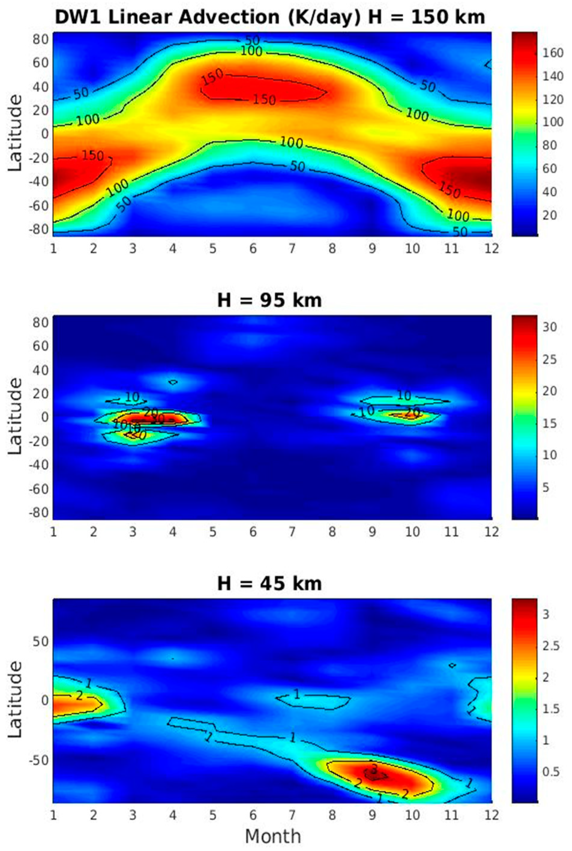
3.3. The Role of the Wave-Mean Flow Interactions (Linear Advection)

Figure 5 shows the seasonal variations of linear advection at 45, 95, and 150 km. At 45 km, in comparison with the adiabatic, short-wave heating and total time tendency (~15 K/day), linear advection is the smallest (3 K/day) and displays a two-peak feature with one located over the equator in December–March and the other in the southern hemisphere (SH) high latitudes during August–November. The seasonal variation of the linear advection does not resemble that of the tide. This implies that linear advection does not play an important role in governing the seasonal variation of the tide at this level.

At 95 km, linear advection has amplitudes of 30 K/day and maximize over the tropical and subtropical regions, similar as the tidal latitudinal structure. It also exhibits similar semiannual variation as the tide. At 150 km, the linear advection has amplitudes of 150 K/day and present similar annual variation as the tide.

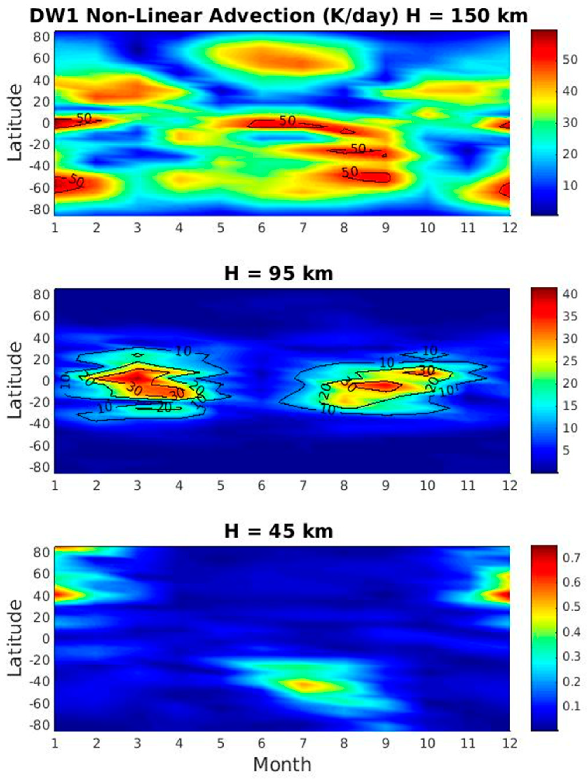
3.4. The Role of the Wave-Wave Interactions (Nonlinear Advection)

Figure 6 shows the seasonal variations of nonlinear advection at 45, 95, and 150 km. At 45 km, in comparison with the adiabatic, short-wave heating and total time tendency (~15 K/day), nonlinear advection has negligible amplitudes of 0.7 K/day. This implies that nonlinear advection does not play an important role in governing the seasonal variation of the tide at this level. At 95 km, nonlinear advection has amplitudes of 40 K/day (slightly larger than the linear advection term) and maximize over the tropical and subtropical regions, similar as the tidal latitudinal structure. It also exhibits similar semiannual variation as the tide. This indicates that nonlinear advection term is important governing the seasonal variation of tide at this level. At 150 km, the nonlinear advection has amplitudes of 50 K/day (one third of the linear advection amplitude), however, it does not present similar annual variation as the tide.

4. Conclusions

With 31.5-year data from eCMAM30 (1979–2010), this paper aims to investigate the roles of linear, nonlinear advection and solar heating in governing the seasonal variations of DW1 in three atmospheric regions: stratosphere, mesosphere, and lower thermosphere (up to 220 km). DW1 is known to have three distinct latitudinal structures and seasonal variations in these atmospheric regions.

In the upper stratosphere (45 km), DW1 T exhibits annual variation and maximizes in the summer. From the analysis of the thermodynamic budget, the short-wave heating is the most important at the middle and high latitudes and excites the tide locally. However, at the equatorial region, both adiabatic and short-wave heating are important. These two terms are out of phase with each other and result in amplitude minimum in the tidal T field. The linear and nonlinear advections do not play important role in governing the seasonal variation of the tide at this level.

In the mesosphere (95 km), DW1 T presents the well-known semiannual variations with stronger amplitude during equinox and weaker amplitude during solstice. Solar heating does not explain the seasonal variation of the tide at this level, where as both linear (tide-mean flow interaction) and nonlinear (tide-wave interaction) advection terms play an important role and exhibit similar seasonal variations as the tide.

In the lower thermosphere (150 km), both the short-wave heating and linear advection play an important role in governing the annual variation of the tide, whereas nonlinear advection does not.

Overall, this study shows the complexity of the main physical mechanisms and departure from the classical tidal theory in modulating the seasonal variations of tides at different regions of the atmosphere. DW1 in the stratosphere is mainly excited in-situ and is dominated by the short-wave heating in the high latitudes, but both the short-wave and adiabatic heating are important in the low latitudes. The seasonal variation of DW1 in the stratosphere is mainly driven radiatively. In the mesosphere, short-wave heating at this level cannot explain the seasonal variation of the tide. The seasonal variation of DW1 in the mesosphere is mainly dynamically driven by wave-wave and wave-mean flow interactions. In the lower thermosphere (130–220 km), both radiative and dynamical process (wave-mean flow interaction) are important in governing the seasonal variation. Despite the above findings, one needs to keep in mind that these conclusions are model specific. Nevertheless, a detailed budget analysis such as this can provide insight into the physical mechanisms that governing the seasonal variation of the tide in a model that can simulate the tide reasonably well in all three regions of the atmosphere.

References

1. Groves, G. Hough components of ozone heating. J. Atmos. Sol. Terr. Phys. 1982, 44, 111–121. [Google Scholar] [CrossRef]
2. Groves, G. Hough components of water vapour heating. J. Atmos. Sol. Terr. Phys. 1982, 44, 281–290. [Google Scholar] [CrossRef]
3. Forbes, J.M. Tidal and planetary waves, The upper mesosphere and lower thermosphere: A review of experiment and theory. Geophys. Monogr. Ser. 1995, 67–87. [Google Scholar] [CrossRef]
4. Hagan, M.; Forbes, J.M. Migrating and nonmigrating diurnal tides in the middle and upper atmosphere excited by tropospheric latent heat release. J. Geophys. Res. 2002, 107, 4754. [Google Scholar] [CrossRef]
5. Hagan, M.; Forbes, J.M. Migrating and nonmigrating semidiurnal tides in the upper atmosphere excited by tropospheric latent heat release. J. Geophys. Res. 2003, 108, 1062. [Google Scholar] [CrossRef]
6. Teitelbaum, H.; Vial, F. On tidal variability induced by nonlinear interaction with planetary waves. J. Geophys. Res. 1991, 96, 14169–14178. [Google Scholar] [CrossRef]
7. Beard, A.; Mitchell, N.; Williams, P.; Kunitake, M. Non-linear interactions between tides and planetary waves resulting in periodic tidal variability. J. Atmos. Sol. Terr. Phys. 1999, 61, 363–376. [Google Scholar] [CrossRef]
8. Angelats i Coll, M.; Forbes, J.M. Nonlinear interactions in the upper atmosphere: The s = 1 and s = 3 nonmigrating semidiurnal tides. J. Geophys. Res. 2002, 107, 1157. [Google Scholar] [CrossRef]
9. Hagan, M.; Roble, R.; Hackney, J. Migrating thermospheric tides. J. Geophys. Res. 2001, 106, 12739–12752. [Google Scholar] [CrossRef] [Green Version]
10. Oberheide, J.; Hagan, M.E.; Richmond, A.D.; Forbes, J.M. Atmospheric Tides. In Encyclopedia of Atmospheric Sciences, 2nd ed.; Elsevier: Amsterdam, The Netherlands, 2015; Volume 2, pp. 287–297. ISBN 9780123822253. [Google Scholar]
11. Williams, P.; Mitchell, N.; Beard, A.; Howells, V.S.C.; Muller, H. The coupling of planetary waves, tides and gravity waves in the mesosphere and lower thermosphere. Adv. Space Res. 1999, 24, 1571–1576. [Google Scholar] [CrossRef]
12. Ortland, D.A.; Alexander, M.J. Gravity wave influence on the global structure of the diurnal tide in the mesosphere and lower thermosphere. J. Geophys. Res. 2006, 111, A10S10. [Google Scholar] [CrossRef]
13. Palo, S.; Forbes, J.M.; Zhang, X.; Russell, J.; Mlynczak, M. An eastward propagating two-day wave: Evidence for nonlinear planetary wave and tidal coupling in the mesosphere and lower thermosphere. Geophys. Res. Lett. 2007, 34, L07807. [Google Scholar] [CrossRef]
14. Agner, R.; Liu, A.Z. Local time variation of gravity wave momentum fluxes and their relationship with the tides derived from LIDAR measurements. J. Atmos. Sol. Terr. Phys. 2015, 135, 136–142. [Google Scholar] [CrossRef] [Green Version]
15. Kazimirovsky, E.; Herraiz, M.; De la Morena, B. Effects on the ionosphere due to phenomena occurring below it. Surv. Geophys. 2003, 24, 139–184. [Google Scholar] [CrossRef]
16. Immel, T.J.; Sagawa, E.; England, S.L.; Henderson, S.B.; Hagan, M.E.; Mende, S.B.; Frey, H.U.; Swenson, C.M.; Paxton, L.J. Control of equatorial ionospheric morphology by atmospheric tides. Geophys. Res. Lett. 2006, 33, L15108. [Google Scholar] [CrossRef]
17. Yamazaki, Y.; Richmond, A.D. A theory of ionospheric response to upward-propagating tides: Electrodynamic effects and tidal mixing effects. J. Geophys. Res. 2013, 118, 5891–5905. [Google Scholar] [CrossRef] [Green Version]
18. Negrea, C.; Zabotin, N.; Bullett, T.; Codrescu, M.; Fuller-Rowell, T. Ionospheric response to tidal waves measured by dynasonde techniques. J. Geophys. Res. 2016, 121, 602–611. [Google Scholar] [CrossRef]
19. McLandress, C. The seasonal variation of the propagating diurnal tide in the mesosphere and lower thermosphere. Part I: The role of gravity waves and planetary waves. J. Atmos. Sci. 2002, 59, 893–906. [Google Scholar] [CrossRef]
20. McLandress, C. The seasonal variation of the propagating diurnal tide in the mesosphere and lower thermosphere. Part II: The role of tidal heating and zonal mean winds. J. Atmos. Sci. 2002, 59, 907–922. [Google Scholar] [CrossRef]
21. Hays, P.B.; Wu, D. HRDI Science Team, Observations of the diurnal tide from space. J. Atmos. Sci. 1994, 51, 3077–3093. [Google Scholar] [CrossRef]
22. Zeng, Z.; Randel, W.; Sokolovskiy, S.; Deser, C.; Kuo, Y.-H.; Hagan, M.; Du, J.; Ward, W.E. Detection of migrating diurnal tide in the tropical upper troposphere and lower stratosphere using the Challenging Minisatellite Payload radio occultation data. J. Geophys. Res. 2008, 113, D03102. [Google Scholar] [CrossRef]
23. Mukhtarov, P.; Pancheva, D.; Andonov, B. Global structure and seasonal and interannual variability of the migrating diurnal tide seen in the SABER/TIMED temperatures between 20 and 120 km. J. Geophys. Res. 2009, 114, A02309. [Google Scholar] [CrossRef]
24. Sakazaki, T.; Fujiwara, M.; Zhang, X.; Hagan, M.; Forbes, J. Diurnal tides from the troposphere to the lower mesosphere as deduced from TIMED/SABER satellite data and six global reanalysis data sets. J. Geophys. Res. 2012, 117, D13108. [Google Scholar] [CrossRef]
25. Smith, A.K. Global dynamics of the MLT. Surv. Geophys. 2012, 33, 1177–1230. [Google Scholar] [CrossRef]
26. Oberheide, J.; Forbes, J.; Zhang, X.; Bruinsma, S. Climatology of upward propagating diurnal and semidiurnal tides in the thermosphere. J. Geophys. Res. 2011, 116, A11306. [Google Scholar] [CrossRef]
27. Forbes, J.M.; Zhang, X.; Bruinsma, S.; Oberheide, J. Sun-synchronous thermal tides in exosphere temperature from CHAMP and GRACE accelerometer measurements. J. Geophys. Res. 2011, 116, A11309. [Google Scholar] [CrossRef]
28. Jones, M., Jr.; Forbes, J.M.; Hagan, M.E.; Maute, A. Impacts of vertically propagating tides on the mean state of the ionosphere-thermosphere system. J. Geophys. Res. Space Phys. 2014, 119, 2197–2213. [Google Scholar] [CrossRef] [Green Version]
29. Siskind, D.E.; Drob, D.P.; Dymond, K.F.; McCormack, J.P. Simulations of the effects of vertical transport on the thermosphere and ionosphere using two coupled models. J. Geophys. Res. Space Phys. 2014, 119, 1172–1185. [Google Scholar] [CrossRef] [Green Version]
30. Lieberman, R.S.; Riggin, D.M.; Ortland, D.A.; Nesbitt, S.W.; Vincent, R.A. Variability of mesospheric diurnal tides and tropospheric diurnal heating during 1997–1998. J. Geophys. Res. 2007, 112, D20110. [Google Scholar] [CrossRef]
31. Akmaev, R. Simulation of large-scale dynamics in the mesosphere and lower thermosphere with the Doppler-spread parameterization of gravity waves: 2. Eddy mixing and the diurnal tide. J. Geophys. Res. 2001, 106, 1205–1213. [Google Scholar] [CrossRef] [Green Version]
32. Hagan, M.; Forbes, J.; Vial, F. On modeling migrating solar tides. Geophys. Res. Lett. 1995, 22, 893–896. [Google Scholar] [CrossRef]
33. Hagan, M.; Burrage, M.D.; Forbes, J.; Hackney, J.; Randel, W.; Zhang, X. GSWM-98: Results for migrating solar tides. J. Geophys. Res. 1999, 104, 6813–6827. [Google Scholar] [CrossRef] [Green Version]
34. McLandress, C. Seasonal variability of the diurnal tide: Results from the Canadian middle atmosphere general circulation model. J. Geophys. Res. 1997, 102, 29747–29764. [Google Scholar] [CrossRef] [Green Version]
35. Lieberman, R.; Ortland, D.; Riggin, D.; Wu, Q.; Jacobi, C. Momentum budget of the migrating diurnal tide in the mesosphere and lower thermosphere. J. Geophys. Res. 2010, 115, D20105. [Google Scholar] [CrossRef]
36. Lu, X.; Liu, H.L.; Liu, A.; Yue, J.; McInerney, J.; Li, Z. Momentum budget of the migrating diurnal tide in the Whole Atmosphere Community Climate Model at vernal equinox. J. Geophys. Res. 2012, 117, D07112. [Google Scholar] [CrossRef]
37. Gan, Q.; Du, J.; Ward, W.E.; Beagley, S.R.; Fomichev, V.I.; Zhang, S.D. Climatology of the diurnal tides from eCMAM30 (1979 to 2010) and its comparison with SABER. Earth Planets Space 2014, 66, 103. [Google Scholar] [CrossRef] [Green Version]
38. Hagan, M.E. Comparative effects of migrating solar sources on tidal signatures in the middle and upper atmosphere. J. Geophys. Res. 1996, 101, 21213–21222. [Google Scholar] [CrossRef]
39. Liu, H.L.; Foster, B.T.; Hagan, M.E.; McInerney, J.M.; Maute, A.; Qian, L.; Richmond, A.D.; Roble, R.G.; Solomon, S.C.; Garcia, R.R.; et al. Thermosphere extension of the Whole Atmosphere Community Climate Model. J. Geophys. Res. 2010, 115, A12302. [Google Scholar] [CrossRef]
40. García-Comas, M.; González-Galindo, F.; Funke, B.; Gardini, A.; Jurado-Navarro, A.; López-Puertas, M.; Ward, W.E. MIPAS observations of longitudinal oscillations in the mesosphere and the lower thermosphere: Climatology of odd-parity daily frequency modes. Atmos. Chem. Phys. 2016, 16, 11019–11041. [Google Scholar] [CrossRef]
41. Beagley, S.R.; McLandress, C.; Fomichev, V.I.; Ward, W.E. Extended Canadian middle atmosphere model. Geophys. Res. Lett. 2000, 27, 2529–2532. [Google Scholar] [CrossRef]
42. Fomichev, V.; Ward, W.E.; Beagley, S.; McLandress, C.; McConnell, J.; McFarlane, N.; Shepherd, T. Extended Canadian Middle Atmosphere Model: Zonal-mean climatology and physical parameterizations. J. Geophys. Res. 2002, 107, ACL 9-1–ACL 9-14. [Google Scholar] [CrossRef]
43. McLandress, C.; Ward, W.E.; Fomichev, V.; Semeniuk, K.; Beagley, S.; McFarlane, N.; Shepherd, T. Large-scale dynamics of the mesosphere and lower thermosphere: An analysis using the extended Canadian Middle Atmosphere Model. J. Geophys. Res. 2006, 111, D17111. [Google Scholar] [CrossRef]
44. Hines, C.O. Doppler-spread parameterization of gravity-wave momentum deposition in the middle atmosphere. 1. Basic formulation. J. Atmos. Sol. Terr. Phys. 1997, 59, 371–386. [Google Scholar] [CrossRef]
45. Hines, C.O. Doppler-spread parameterization of gravity-wave momentum deposition in the middle atmosphere. 2. Broad and quasi monochromatic spectra, and implementation. J. Atmos. Sol. Terr. Phys. 1997, 59, 387–400. [Google Scholar] [CrossRef]
46. Du, J.; Ward, W.E.; Oberheide, J.; Nakamura, T.; Tsuda, T. Semidiurnal tides from the extended Canadian Middle Atmosphere Model (CMAM) and comparisons with TIMED Doppler interferometer (TIDI) and meteor radar observations. J. Atmos. Sol. Terr. Phys. 2007, 69, 2159–2202. [Google Scholar] [CrossRef]
47. Du, J.; Ward, W.E. Terdiurnal tide in the extended Canadian Middle Atmospheric Model (CMAM). J. Geophys. Res. 2010, 115, D24106. [Google Scholar] [CrossRef]
48. Du, J.; Ward, W.E.; Cooper, F. The character of polar tidal signatures in the extended Canadian Middle Atmosphere Model. J. Geophys. Res. 2014, 119, 5928–5948. [Google Scholar] [CrossRef] [Green Version]
49. de Grandpré, J.; Beagley, S.R.; Fomichev, V.I.; Griffioen, E.; McConnell, J.C.; Medvedev, A.S.; Shepherd, T.G. Ozone climatology using interactive chemistry: Results from the Canadian Middle Atmosphere Model. J. Geophys. Res. 2000, 105, 26475–26491. [Google Scholar] [CrossRef] [Green Version]
50. Beagley, S.R.; Boone, C.D.; Fomichev, V.I.; Jin, J.J.; Semeniuk, K.; McConnell, J.C.; Bernath, P.F. First multi-year occultation observations of CO2 in the MLT by ACE satellite: Observations and analysis using the extended CMAM. Atmos. Chem. Phys. 2010, 10, 1133–1153. [Google Scholar] [CrossRef]
51. Shepherd, M.G.; Beagley, S.R.; Fomichev, V.I. Stratospheric warming influence on the mesosphere/lower thermosphere as seen by the extended CMAM. Ann. Geophys. 2014, 32, 589–608. [Google Scholar] [CrossRef] [Green Version]
52. Dee, D.; Uppala, S.; Simmons, A.; Berrisford, P.; Poli, P.; Kobayashi, S.; Andrae, U.; Balmaseda, M.; Balsamo, G.; Bauer, P. The ERA-Interim reanalysis: Configuration and performance of the data assimilation system. Q. J. R. Meteorol. Soc. 2011, 137, 553–597. [Google Scholar] [CrossRef]
53. McLandress, C.; Scinocca, J.F.; Shepherd, T.G.; Reader, M.C.; Manney, G.L. Dynamical control of the mesosphere by orographic and nonorographic gravity wave drag during the extended northern winters of 2006 and 2009. J. Atmos. Sci. 2013, 70, 2152–2169. [Google Scholar] [CrossRef]
54. Forster, P.M.; Fomichev, V.I.; Rozanov, E.; Cagnazzo, C.; Jonsson, A.I.; Langematz, U.; Fomin, B.; Iacono, M.J.; Mayer, B.; Mlawer, E.; et al. Evaluation of radiation scheme performance within chemistry climate models. J. Geophys. Res. 2011, 116. [Google Scholar] [CrossRef] [Green Version]
55. Semeniuk, K.; Fomichev, V.I.; McConnell, J.C.; Fu, C.; Melo, S.M.L.; Usoskin, I.G. Middle atmosphere response to the solar cycle in irradiance and ionizing particle precipitation. Atmos. Chem. Phys. 2011, 11, 5045–5077. [Google Scholar] [CrossRef] [Green Version]
56. Chapman, S.; Lindzen, R.S. Atmospheric Tides: Thermal and Gravitational; Gordon and Breach: New York, NY, USA, 1970; 200p. [Google Scholar]
57. Hagan, M.E.; Häusler, K.; Lu, G.; Forbes, J.M.; Zhang, X. Upper thermospheric responses to forcing from above and below during 1–10 April 2010: Results from an ensemble of numerical simulations. J. Geophys. Res. Space Phys. 2015, 120, 3160–3174. [Google Scholar] [CrossRef]
Figure 1. Climatological mean latitude-height structure of DW1 (the migrating diurnal tide) amplitude in the stratosphere (bottom panel), mesosphere (middle panel) and thermosphere (top panel) for temperature T (K) in March from the eCMAM30 (1979–2010).
Atmosphere 09 00440 g001
Figure 2. Seasonal variations of the time tendency (K/day) on the left-hand-side (LHS) of thermodynamic budget Equation (1) for DW1 at 45, 95 and 150 km. The LHS is simply the DW1 T amplitude times 2pi.
Atmosphere 09 00440 g002
Figure 3. Seasonal variations of the adiabatic heating, short-wave heating, and the sum of adiabatic and short-wave heating (K/day) on the right-hand-side (RHS) of thermodynamic budget Equation (1) for DW1 at 45 km.
Atmosphere 09 00440 g003
Figure 4. Top two panels: Seasonal variations of the short-wave heating (K/day) on the right-hand-side (RHS) of thermodynamic budget Equation (1) for DW1 at 95 and 150 km. Bottom two panels: seasonal variations of the short-wave heating as a function of height at the Equator and 35° N.
Atmosphere 09 00440 g004
Figure 5. Seasonal variations of the linear advection term (wave-mean flow interaction) (K/day) on the right-hand-side (RHS) of thermodynamic budget Equation (1) for DW1 at 45, 95 and 150 km.
Atmosphere 09 00440 g005
Figure 6. Same as Figure 5, but for the nonlinear advection term (wave-wave interaction).
Atmosphere 09 00440 g006