The Impacts of Smoke Emitted from Boreal Forest Wildfires on the High Latitude Radiative Energy Budget—A Case Study of the 2002 Yakutsk Wildfires


Abstract
1. Introduction
2. Methodology
2.1. Model Configuration
2.2. Remote Sensing Data
3. Results: Assessment of the Impact of Smoke on Radiation
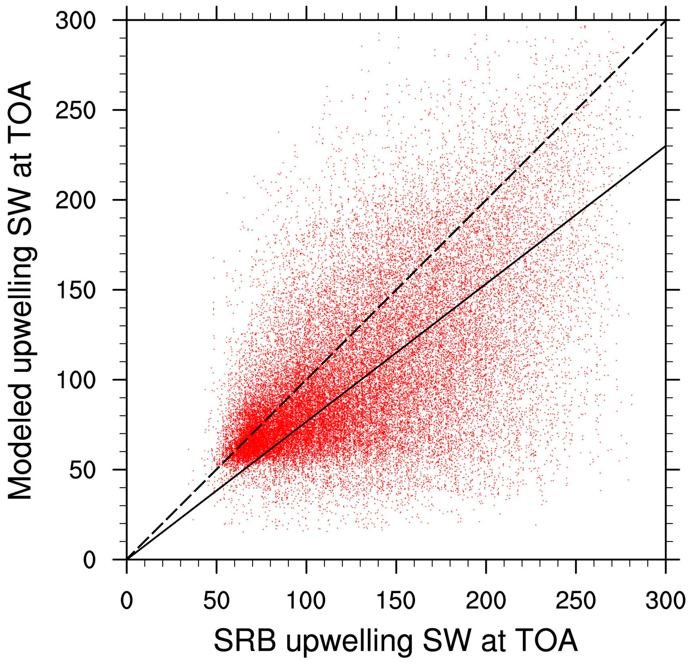
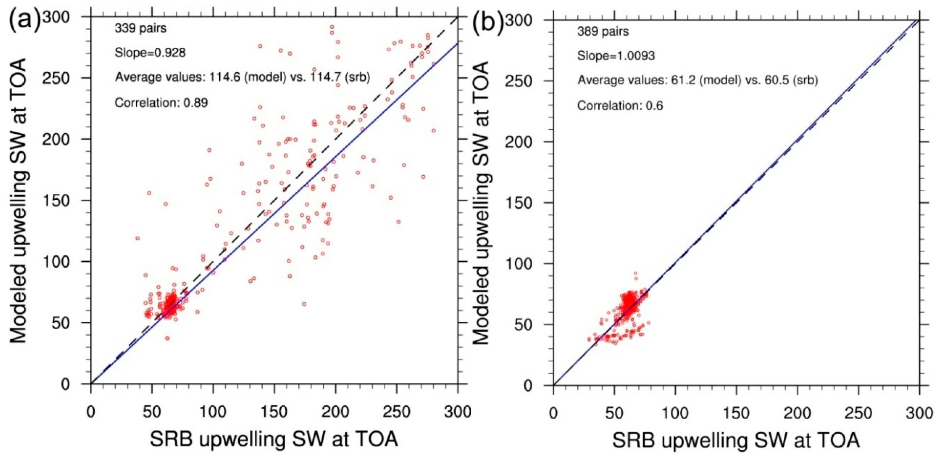
3.1. Comporison of Modeled Radiative Fluxs against the SRB Dataset
3.2. The Impact of Smoke on Radiative Fluxes during the Fire Period 1
3.3. The Impact of Smoke on Radiative Fluxes during the Fire Period 2
4. Discussion and Conclusions
Author Contributions
Funding
Conflicts of Interest
References
- Forkel, R.; Balzarini, A.; Baro, R.; Bianconi, R.; Curci, G.; Jimenez-Guerrero, P.; Hirtl, M.; Honzak, L.; Lorenz, C.; Im, U.; et al. Analysis of the WRF-Chem contributions to AQMEII phase 2 with respect to aerosol radiative feedbacks on meteorology and pollutant distributions. Atmos. Environ. 2015, 115, 630–645. [Google Scholar] [CrossRef]
- Kong, X.; Forkel, R.; Sokhi, R.S.; Suppan, P.; Baklanov, A.; Gauss, M.; Brunner, D.; Baro, R.; Balzarini, A.; Chemel, C.; et al. Analysis of meteorology-chemistry interactions during air pollution episodes using online coupled models within AQMEII phase-2. Atmos. Environ. 2015, 115, 527–540. [Google Scholar] [CrossRef]
- Palacios-Pena, L.; Baro, R.; Baklanov, A.; Balzarini, A.; Brunner, D.; Forkel, R.; Hirtl, M.; Honzak, L.; Lopez-Romero, J.M.; Montavez, J.P.; et al. An assessment of aerosol optical properties from remote-sensing observations and regional chemistry climate coupled models over Europe. Atmos. Chem. Phys. 2018, 18, 5021–5043. [Google Scholar] [CrossRef]
- Stone, R.S.; Anderson, G.P.; Shettle, E.P.; Andrews, E.; Loukachine, K.; Dutton, E.; Schaaf, C.; Roman, M.O., III. Radiative impact of boreal smoke in the Arctic: Observed and modeled. J. Geophys. Res. 2008, 113, D14S16. [Google Scholar] [CrossRef]
- Carslaw, K.S.; Boucher, O.; Spracklen, D.V.; Mann, G.W.; Rae, J.G.L.; Woodward, S.; Kulmala, M. A review of natural aerosol interactions and feedbacks within the Earth system. Atmos. Chem. Phys. 2010, 10, 1701–1737. [Google Scholar] [CrossRef]
- Penner, J.E.; Dickinson, R.E.; O’Neill, C.A. Effects of aerosol from biomass burning on the global radiation budget. Science 1992, 256, 1432–1434. [Google Scholar] [CrossRef] [PubMed]
- Andreae, M.O.; Rosenfeld, D. Aerosol–cloud–precipitation interactions, part 1. The nature and sources of cloud-active aerosols. Earth-Sci. Rev. 2008, 89, 13–41. [Google Scholar] [CrossRef]
- Jiang, Y.; Lu, Z.; Liu, X.; Qian, Y.; Zhang, K.; Wang, Y.; Yang, X.-Q. Impacts of global open-fire aerosols on direct radiative, cloud and surface-albedo effects simulated with CAM5. Atmos. Chem. Phys. 2016, 16, 14805–14824. [Google Scholar] [CrossRef]
- Gorbatenko, V.P.; Ippolitov, I.I.; Podnebesnykh, N.V. Atmospheric Circulation over Western Siberia in 1976–2004. Russ. Meteorol. Hydrol. 2007, 32, 301–306. [Google Scholar] [CrossRef]
- Péré, J.C.; Bessagnet, B.; Mallet, M.; Waquet, F.; Chiapello, I.; Minvielle, F.; Pont, V.; Menut, L. Direct radiative effect of the Russian wildfires and its impact on air temperature and atmospheric dynamics during August 2010. Atmos. Chem. Phys. 2014, 14, 1999–2013. [Google Scholar] [CrossRef]
- Toll, V.; Reis, K.; Ots, R.; Kaasik, M.; Männik, A.; Prank, M.; Sofiev, M. SILAM and MACC reanalysis aerosol data used for simulating the aerosol direct radiative effect with the NWP model HARMONIE for summer 2010 wildfire case in Russia. Atmos. Environ. 2015, 121, 75–85. [Google Scholar] [CrossRef]
- Lu, Z.; Sokolik, I.N. Examining the impact of smoke on frontal clouds and precipitation during the 2002 Yakutsk wildfires using the WRF-Chem-SMOKE model and satellite data. J. Geophys. Res. Atmos. 2017, 122, 12765–12785. [Google Scholar] [CrossRef]
- Lu, Z.; Sokolik, I.N. The effect of smoke emission amount on changes in cloud properties and precipitation: A case study of Canadian boreal wildfires of 2007. J. Geophys. Res. Atmos. 2013, 118, 11777–11793. [Google Scholar] [CrossRef]
- Grell, G.A.; Peckham, S.E.; Schmitz, R.; McKeen, S.A.; Frost, G.; Skamarock, W.C.; Eder, B. Fully coupled “online” chemistry within the WRF model. Atmos. Environ. 2005, 39, 6957–6975. [Google Scholar] [CrossRef]
- Zaveri, R.A.; Easter, R.C.; Fast, J.D.; Peters, L.K. Model for Simulating Aerosol Interactions and Chemistry (MOSAIC). J. Geophys. Res. 2008, 113, D13204. [Google Scholar] [CrossRef]
- Ichoku, C.; Kaufman, Y.J. A method to derive smoke emission rates from MODIS fire radiative energy measurements. IEEE Trans. Geosci. Remote Sens. 2005, 43, 2636–2649. [Google Scholar] [CrossRef]
- Chou, M.D.; Suarez, M.J.; Ho, C.H.; Yan, M.M.H.; Lee, K.T. Parameterizations for cloud overlapping and shortwave single-scattering properties for use in general circulation and cloud ensemble models. J. Clim. 1998, 11, 202–214. [Google Scholar] [CrossRef]
- Fast, J.D.; Gustafson, W.I., Jr.; Easter, R.C.; Zaveri, R.A.; Barnard, J.C.; Chapman, E.G.; Grell, G.A.; Peckham, S.E. Evolution of ozone, particulates, and aerosol direct radiative forcing in the vicinity of Houston using a fully coupled meteorology-chemistry-aerosol model. J. Geophys. Res. 2006, 111, D21305. [Google Scholar] [CrossRef]
- Morrison, H.; Curry, J.A.; Khvorostyanov, V.I. A new double-moment microphysics scheme for application in cloud and climate models. Part I: Description. J. Atmos. Sci. 2005, 62, 1665–1677. [Google Scholar] [CrossRef]
- Pinker, R.T.; Laszlo, I. Modeling surface solar irradiance for satellite applications on a global scale. J. Appl. Meteorol. 1992, 31, 194–211. [Google Scholar] [CrossRef]
- Gupta, S.K.; Kratz, D.P.; Stackhouse, P.W., Jr.; Wilber, A.C. The Langley Parameterized Shortwave Algorithm (LPSA) for Surface Radiation Budget Studies; NASA Langley Research Center: Hampton, VA, USA, 2001.
- Fu, Q.; Liou, K.-N.; Cribb, M.C.; Charlock, T.P.; Grossman, A. Multiple scattering parameterization in thermal infrared radiative transfer. J. Atmos. Sci. 1997, 54, 2799–2812. [Google Scholar] [CrossRef]
- Nam, C.; Bony, S.; Dufresne, J.-L.; Chepfer, H. The ‘too few, too bright’ tropical low-cloud problem in CMIP5 models. Geophys. Res. Lett. 2012, 39, L21801. [Google Scholar] [CrossRef]
- Wu, L.; Su, H.; Jiang, J.H. Regional simulations of deep convection and biomass burning over South America: 2. Biomass burning aerosol effects on clouds and precipitation. J. Geophys. Res. 2011, 116, D17209. [Google Scholar] [CrossRef]


© 2018 by the authors. Licensee MDPI, Basel, Switzerland. This article is an open access article distributed under the terms and conditions of the Creative Commons Attribution (CC BY) license (http://creativecommons.org/licenses/by/4.0/).
Share and Cite
Lu, Z.; Sokolik, I.N. The Impacts of Smoke Emitted from Boreal Forest Wildfires on the High Latitude Radiative Energy Budget—A Case Study of the 2002 Yakutsk Wildfires. Atmosphere 2018, 9, 410. https://doi.org/10.3390/atmos9100410
Lu Z, Sokolik IN. The Impacts of Smoke Emitted from Boreal Forest Wildfires on the High Latitude Radiative Energy Budget—A Case Study of the 2002 Yakutsk Wildfires. Atmosphere. 2018; 9(10):410. https://doi.org/10.3390/atmos9100410
Chicago/Turabian StyleLu, Zheng, and Irina N. Sokolik. 2018. "The Impacts of Smoke Emitted from Boreal Forest Wildfires on the High Latitude Radiative Energy Budget—A Case Study of the 2002 Yakutsk Wildfires" Atmosphere 9, no. 10: 410. https://doi.org/10.3390/atmos9100410
APA StyleLu, Z., & Sokolik, I. N. (2018). The Impacts of Smoke Emitted from Boreal Forest Wildfires on the High Latitude Radiative Energy Budget—A Case Study of the 2002 Yakutsk Wildfires. Atmosphere, 9(10), 410. https://doi.org/10.3390/atmos9100410