1. Introduction
The southeastern Tibetan Plateau (SETP) plays a pivotal role in regulating the Asian monsoon system and the regional hydrological cycle [
1,
2,
3,
4]. This region encompasses the Tsangpo Grand Canyon—the world’s deepest canyon—which serves as a critical conduit for moisture transport from the Indian Ocean into the plateau interior [
5,
6,
7]. Its steep terrain, strong land–atmosphere interactions, and exposure to moist air masses transported by the Indian Summer Monsoon make the region highly susceptible to intense and spatially heterogeneous precipitation. Extreme rainstorm events in this area frequently trigger landslides, debris flows, and flash floods, posing substantial risks to local ecosystems and human activities [
8]. Such risks underscore the need for a better understanding of the characteristics of extreme precipitation over SETP.
Where surface observations are sparse, numerical modeling offers the principal avenue for investigating precipitation over TP. Long-term Weather Research and Forecasting (WRF) model simulations at grid spacings of 10–30 km have successfully reproduced the large-scale precipitation climatology of the TP, although their performance remains sensitive to the choice of cumulus parameterization [
9,
10,
11]. This sensitivity largely stems from the reliance on parameterized convection, which constrains the representation of processes over the steep orography of the SETP and thereby leads to displaced precipitation maxima, a diurnal cycle that occurs several hours too early, and a loss of fine-scale spatial structure [
12,
13,
14]. Convection-Permitting Simulations (CPMs; 1–4 km) alleviate these deficiencies by explicitly resolving deep convection. Over TP, they have been shown to reduce wet bias, improve the representation of the diurnal cycle, and better capture sub-daily precipitation characteristics [
7,
15,
16,
17,
18]. The recent development of a kilometer-scale ensemble (2.2–4 km) for the Third Pole represents a further step toward explicitly resolving convection at regional scales [
19]. Computational cost, however, has constrained most CPM studies over TP to simulation periods ranging from individual storm events to one or two seasons. A multi-year CPM enables robust estimation of return levels for localized extreme rainfall, which is essential for infrastructure design and flood risk assessment, yet unattainable from short, coarse-resolution simulations.
Estimating return levels for extreme precipitation from short CPM simulations means inferring distribution tails from limited samples. The conventional approach fits a Generalized Extreme Value (GEV) distribution to annual maxima [
20]. Short records leave too few block maxima for stable tail parameter estimation, and the resulting uncertainty intervals are too wide for the 50- or 100-year events that engineering design requires [
21,
22]. Rather than discarding all but the largest event each year, the Metastatistical Extreme Value (MEV) framework models the distribution of all wet events above a threshold and combines that distribution with the annual event count to estimate return levels [
23]. SMEV, a simplified variant, pools wet events across all years to fit a single Weibull distribution and groups them by the underlying physical process to accommodate non-stationarities [
24,
25]. This pooling produces more stable tail estimates than GEV when the record spans only a decade or two. SMEV has been used for daily and subdaily precipitation in Mediterranean, alpine, and monsoon climates [
26,
27,
28]. More closely related to the present study, Dallan et al. [
29] applied SMEV on ten years of 2.2 km CPM output over the Italian Alps, and found that CPM–SMEV can reproduce observed return periods for hourly precipitation over complex terrain. Formetta et al. [
30] extended the same CPM–SMEV framework to estimate return levels at ungauged locations, confirming that the approach remains reliable even with a ten-year record.
In the present work, we apply SMEV to ten years of 1 km WRF simulations over SETP to estimate daily return levels up to 100 years. We evaluate these estimates against satellite-based precipitation retrievals and a regional atmospheric reanalysis, both of which represent the region at substantially coarser resolution. This study investigates the ability of SMEV to produce reliable return-level estimates for daily precipitation using only a decade of convection-resolving model output. It also examines whether 1 km CPM data provides additional information on extreme precipitation over SETP that is not represented in satellite-based products and regional reanalyses at coarser spatial resolution.
3. Methodology
3.1. Theoretical Foundation of SMEV
Independent ordinary precipitation events are first identified from a continuous record using an inter-event time criterion to ensure approximate independence. Let denote the ordinary events within a year, where is the number of events. The events are assumed to be independent and identically distributed (i.i.d.), where denotes the cumulative distribution function of a generic event . The annual maximum is defined as .
Conditioned on a fixed number of events
, the probability that the annual maximum does not exceed a threshold y is given by the following:
In practice, however, the number of events varies from year to year and is treated as a random variable. Following the SMEV framework,
is assumed to follow a Poisson distribution with rate
, representing the average number of events per year. The unconditional distribution of
is therefore obtained by averaging the conditional distribution over all possible values of
:
Under the Poisson assumption, this expression simplifies to the following closed form:
with
where a Weibull distribution is adopted for modeling the ordinary event magnitudes, as recommended in the SMEV framework [
24,
25];
and
denote the scale and shape parameters. By pooling all ordinary events across the 10-year record to fit these parameters, SMEV increases the effective sample size by an order of magnitude compared to traditional annual-maximum methods, which is crucial for achieving stable tail estimates from short-duration CPM simulations.
3.2. Identification of Ordinary Precipitation Events
Here, we restrict our analysis to the daily scale because only daily rain gauge observations are openly accessible. At this scale, ordinary events are defined as all individual wet days exceeding a prescribed threshold within a given year, following common practice in the SMEV framework [
24]. While subdaily scales often employ an inter-event time criterion to ensure independence between individual storms, at the daily resolution, the use of wet days has been shown to provide stable tail estimates and effectively capture extreme-value behavior in various estimates, including monsoon-influenced regions [
25]. Following common practice, we adopt a threshold of 1 mm/d to separate precipitation occurrence from dry conditions [
34,
35]. Within the SMEV framework, only the upper tail of the ordinary event distribution is used, defined by a tail quantile (
) that serves as a hyperparameter dependent on regional climatology. Because our dataset covers only wet-season months, ordinary events from the dry season are necessarily absent. However, since SMEV estimates are driven by upper-tail extremes that occur predominantly during the wet season, the information loss associated with missing dry-season ordinary events is expected to be small. Calibrating the tail quantile against in situ rain gauge observations further ensures that the wet-season tail adequately represents the extreme-value behavior of interest.
3.3. Evaluation Metrics
Three metrics quantify the agreement between gridded precipitation products and rain gauge observations. The Pearson correlation coefficient (R) measures the linear association between simulated and observed annual maxima:
where
and
denote gridded and observed precipitation values, respectively, and
is the number of values. With six rain-gauge stations and ten years of simulation data,
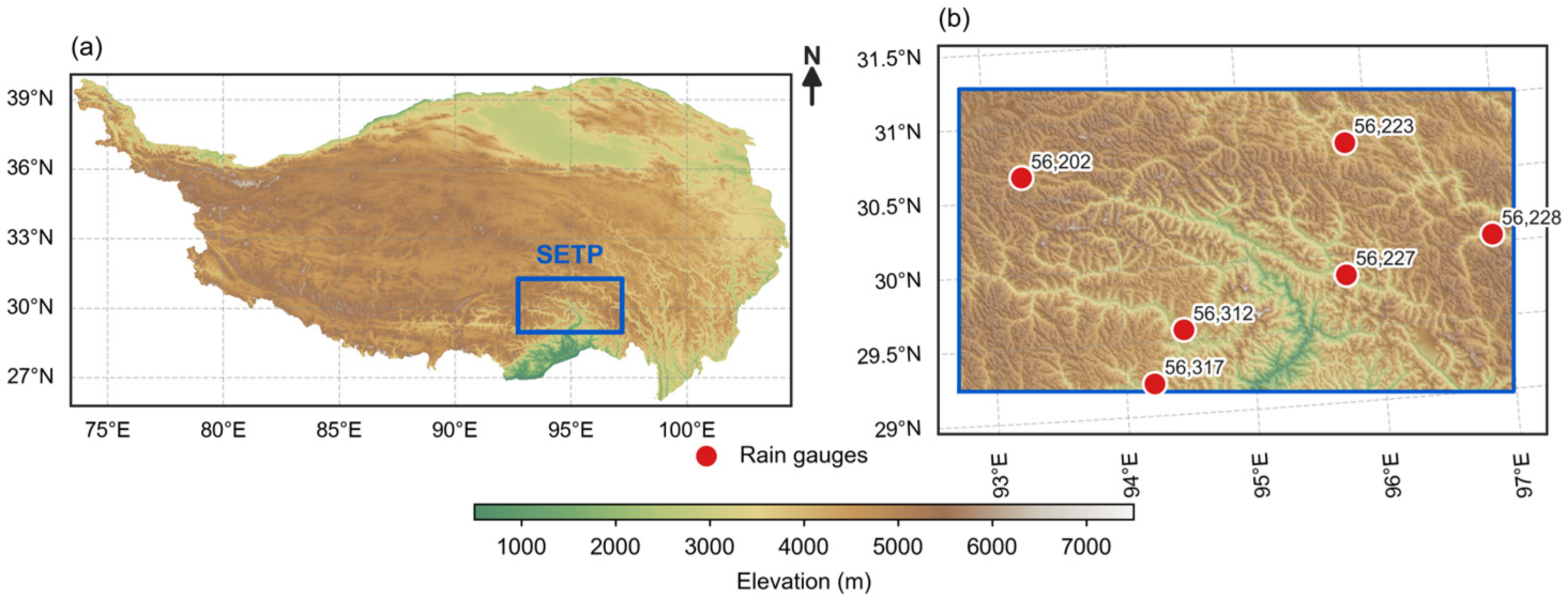
represents the total population of 60 annual maxima points used in the scatterplot analysis. Gridded data were analyzed at the corresponding station locations using the nearest-neighbor method for all six CMA stations.
The root mean square error (RMSE, mm d
−1) captures the overall deviation in magnitude:
Percent bias (PBIAS, %) indicates systematic over- or under-estimation:
3.4. Approach Implementation
The integration of WRF-1 km simulation data into the SMEV framework follows a three-step pipeline. First, the raw hourly precipitation output is aggregated into daily totals (20:00 to 20:00 UTC+8) to ensure temporal consistency with the benchmark CMA rain gauges. Second, gridded precipitation values are extracted at the rain-gauge locations using the nearest neighbor interpolation method based on in situ observations from the 2012–2021 period. The tail quantile (τ) is determined through a systematic grid search over the range [0.05, 0.95] with an interval of 0.05. The optimal τ is identified by minimizing PBIAS between SMEV-estimated return levels and GEV-derived observational benchmarks across multiple standard return periods (2-, 5-, 10-, 20-, and 50-year). For each gridded product, τ is selected by minimizing PBIAS across the full gauge network. This procedure yields a single, regionally uniform hyperparameter per dataset, ensuring that the modeled distribution tail is constrained by physically consistent extreme-value behavior. Third, the SMEV framework is applied pixel-by-pixel across the entire SETP domain. For each grid cell, the two-parameter Weibull distribution is fitted to the ordinary events exceeding the optimized regional using the method of least squares, enabling the consistent spatial mapping of return levels. To quantify sampling uncertainty, we implement a block bootstrap approach with 1000 replicates, resampling entire years with replacement. This same SMEV pipeline is applied to IMERG and HAR v2 using their respective regional τ values to highlight the added value of the 1 km CPM.
4. Results
4.1. Comparison of Annual Maxima
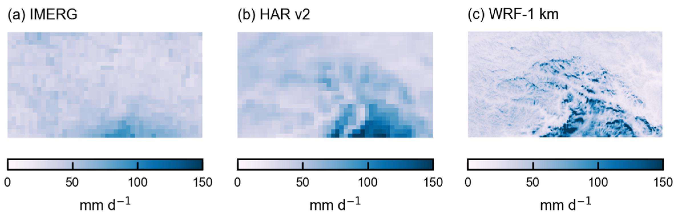
Figure 2 compares the spatial distribution of mean annual maxima of precipitation derived from IMERG, HAR v2, and WRF-1 km. A spatial pattern of extreme precipitation tightly anchored to terrain is revealed by WRF-1 km (
Figure 2c). The ten-year mean annual maximum is substantially higher on the windward slopes of the eastern Himalayas—particularly near Namcha Barwa and along the Yarlung Tsangpo Grand Canyon—than on the leeward Tibetan Plateau above 4500 m and adjacent sheltered valleys. This pronounced windward–leeward contrast is consistent with strong orographic forcing, whereby moist southwesterly monsoon air is lifted along steep escarpments, enhancing precipitation over exposed slopes while subsidence and moisture depletion suppress precipitation over the plateau interior and leeward regions [
5,
6,
7]. WRF-1 km resolves this structure as sharp precipitation gradients across individual ridgelines, with local differences exceeding a factor of two over short distances, rather than a smooth large-scale decrease. In contrast, neither HAR v2 (~10 km) nor IMERG (~10 km) reproduces this terrain-controlled contrast. HAR v2 smooths the canyon-scale maximum into a broad plateau-wide enhancement, attenuating the localized peak within the Tsangpo Grand Canyon and yielding elevated precipitation above ~4000 m. This behavior likely reflects the combined effects of coarse resolution and parameterized convection, which reduce spatial variability and produce a smoother precipitation field over complex terrain [
36]. IMERG exhibits an even more homogenized pattern, with substantially lower peak intensities than WRF-1 km and no clear separation between windward slopes and leeward valleys.
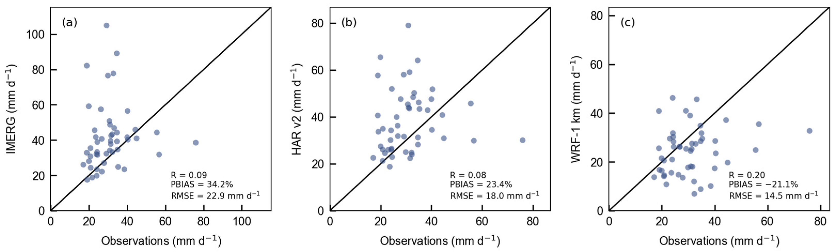
Figure 3 further evaluates these differences against in situ observations. WRF-1 km exhibits the highest correlation (R = 0.20) and lowest RMSE (14.5 mm d
−1) among the tested products, despite a negative bias (PBIAS = −21.1%) indicative of underestimation of the highest extremes. While an R of 0.20 indicates a weak linear correspondence in point-by-point matching of annual maxima, it nonetheless represents a modest improvement over the negligible correlations found in HAR v2 (R = 0.08) and IMERG (R = 0.09). This low correlation underscores the inherent difficulty of capturing the precise timing and location of localized convective events within extreme mountainous terrain, which remains a significant challenge for numerical models. In contrast, both coarse-resolution products exhibit weak correspondence with observations. IMERG performs poorest (RMSE = 22.9 mm d
−1; PBIAS = 34.2%), systematically overestimating moderate events while failing to capture higher extremes, resulting in inflated magnitudes but low fidelity to variability. The wet bias of IMERG at rain gauge locations does not contradict the low rainfall observed around the Yarlung Tsangpo Grand Canyon, mainly because the rain gauges are sparsely distributed, and none are located within the canyon. HAR v2 shows marginal improvement over IMERG in overall magnitude (RMSE = 18.0 mm d
−1; PBIAS = 23.4%) but retains similarly low correlation and substantial scatter.
Table 1 presents station-specific evaluation metrics for the JJAS annual maxima to account for potential error compensation. WRF-1 km remains the most accurate product across all locations, maintaining its performance advantage notwithstanding minor discrepancies at individual stations.
Collectively, these results reveal a consistent error structure: coarse-resolution products tend to overestimate mean annual maxima while poorly representing variability, whereas WRF-1 km reduces overall error and better captures variability but underestimates peak intensities. This contrast underscores the importance of resolving terrain-induced processes for accurately representing extreme precipitation in complex mountainous regions.
4.2. SMEV Return-Level Estimates at Gauge Locations
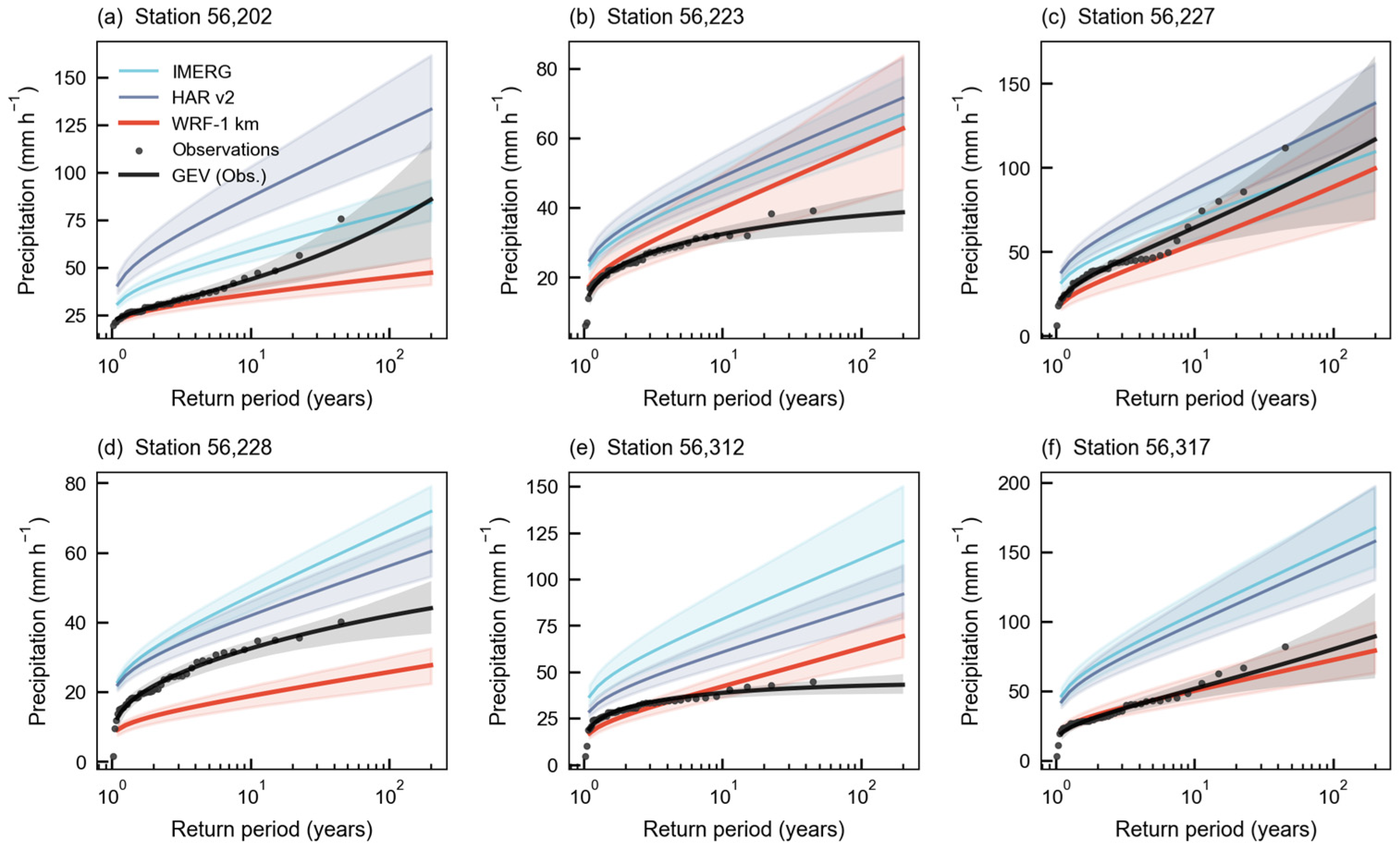
Figure 4 presents the SMEV return-level curves and associated 90% bootstrap confidence intervals (CIs) at each gauge station for the three datasets, using individually calibrated tail quantiles. The tail quantile
differs substantially across products:
= 0.55 for WRF-1 km, meaning roughly 45% of wet days contribute to the Weibull tail fit, compared with
= 0.10 for both HAR v2 and IMERG, where the top 90% of wet days are retained. This contrast reflects differences in tail structure, with WRF-1 km supporting a more stable extreme-value regime, while HARv2 and IMERG require larger samples to constrain the Weibull fit.
To provide a rigorous benchmark, we estimated return levels from the station observations using the GEV distribution applied to the full 1955–2021 period. Across the station network, WRF-1 km SMEV estimates align with the independent statistical fits derived from the full observational record. In contrast, HARv2 and IMERG systematically overestimate return levels and exhibit substantially wider confidence intervals. As shown at Station 56,312 (
Figure 4e), where the observed 50-year return level is 51.6 mm d
−1. WRF-SMEV estimates 57.1 mm d
−1 (CI: 47.1–68.9 mm d
−1), enclosing the observation, whereas HARv2 (78.1 mm d
−1; CI: 65.2–94.4 mm d
−1) and IMERG (101.9 mm d
−1; CI: 80.8–129.4 mm d
−1) overestimate it by ~50% and nearly a factor of two, respectively. Despite this overall skill, WRF exhibits localized dry biases at a few stations (e.g., Stations 56,202 and 56,228;
Figure 4a,d), where observed extremes exceed the predicted confidence bounds. The contrasting behavior among datasets arises from the interaction between intrinsic biases and tail sampling. For both HARv2 and IMERG, systematic wet biases propagate into the Weibull fit (
Figure 3), leading to inflated return-level estimates. To mitigate this bias, a low tail quantile (
τ = 0.10) is adopted, retaining a large fraction of events. This suggests that the SMEV approach can provide a conservative or representative estimation even when point-by-point event matching shows a dry bias. However, despite the enlarged sample, the fitted tail remains sensitive to the highest-intensity events, which exert disproportionate control on the distribution. This results in an artificially heavy tail and a rapid divergence from observations beyond ~20-year return periods.
4.3. Spatial SMEV Return-Level Maps
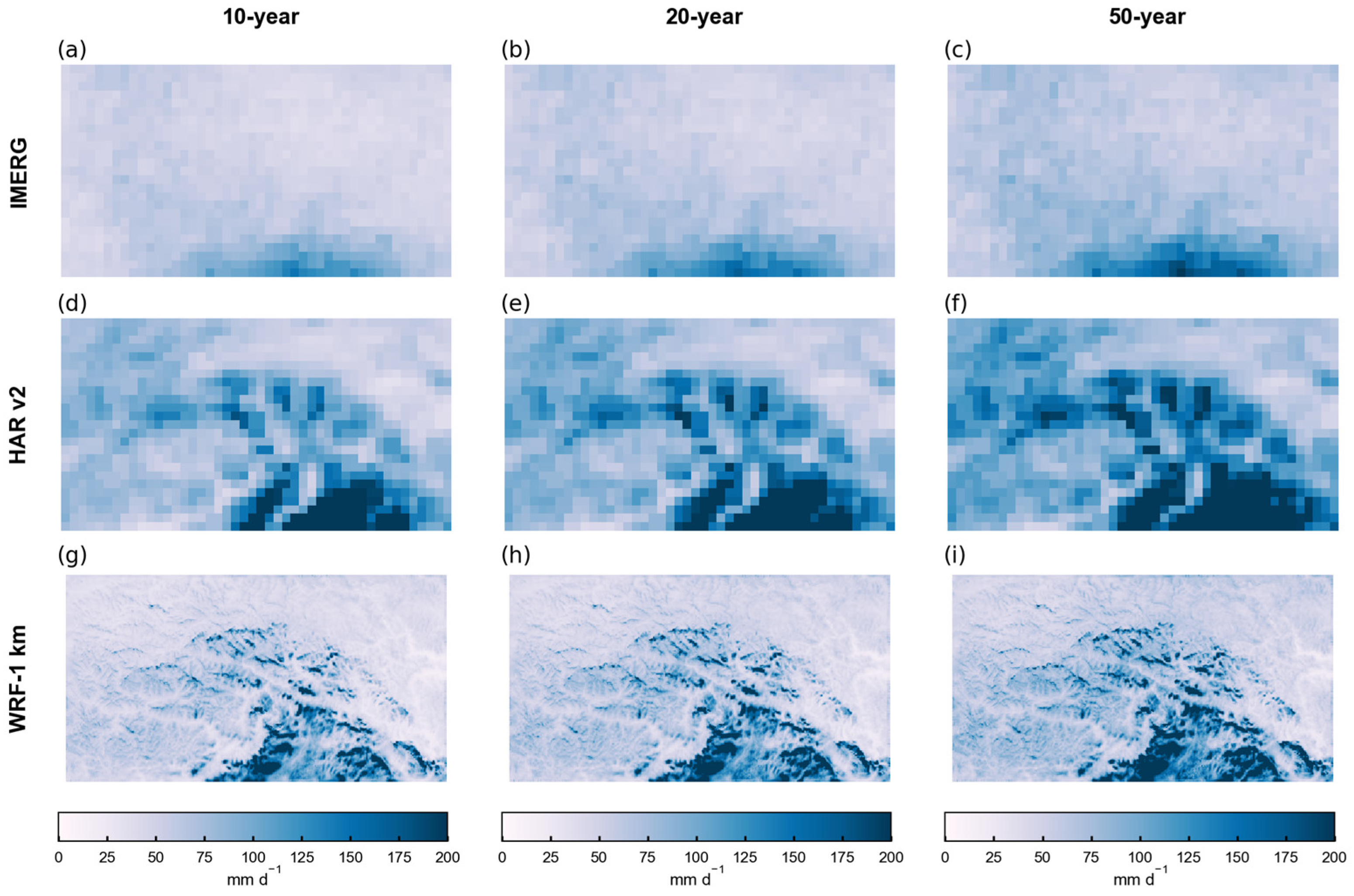
Figure 5 shows the spatial distribution of SMEV-based return levels for multiple return periods across the three gridded precipitation datasets. Instead of deriving the SMEV tail quantiles directly from the gridded precipitation products, the upper-tail quantile parameters were calibrated using sparse in situ observations when fitting the Weibull distribution. This strategy was adopted to reduce the systematic bias introduced by coarse-resolution gridded data, which tend to spatially smooth short-duration precipitation extremes and consequently underestimate upper-tail behavior. Although the sparse gauge network inevitably introduces sampling uncertainty, station-based calibration provides more realistic local tail information than grid-derived estimates alone. Therefore, the SMEV framework prioritizes reducing systematic bias in extreme precipitation estimation, particularly over topographically complex terrain where gridded products commonly exhibit excessive spatial homogenization of extremes. While all products exhibit a consistent intensification of extremes with increasing return period, the WRF-1 km simulations (
Figure 5g–i) demonstrate a markedly superior fidelity in resolving fine-scale spatial heterogeneity compared to the relatively homogenized patterns in IMERG (
Figure 5a–c) and HAR v2 (
Figure 5d–f). WRF-1 km effectively captures distinct orographic signatures and localized “hotspots” of extreme precipitation, with 50-year return levels exceeding 175 mm d
−1 in topographically complex regions. These extreme values are primarily localized within the Tsangpo Grand Canyon, which serves as a critical pathway for water vapor transport from the Indian summer monsoon into the plateau interior. The canyon’s unique funnel-shaped topography and steep windward escarpments trigger intense orographic lifting of moist air masses. In contrast, the coarser datasets exhibit significant spatial smoothing, which leads to an underestimation of localized peak intensities—a bias that remains evident despite the SMEV-based tail calibration.
4.4. Elevation Dependency of Return Levels
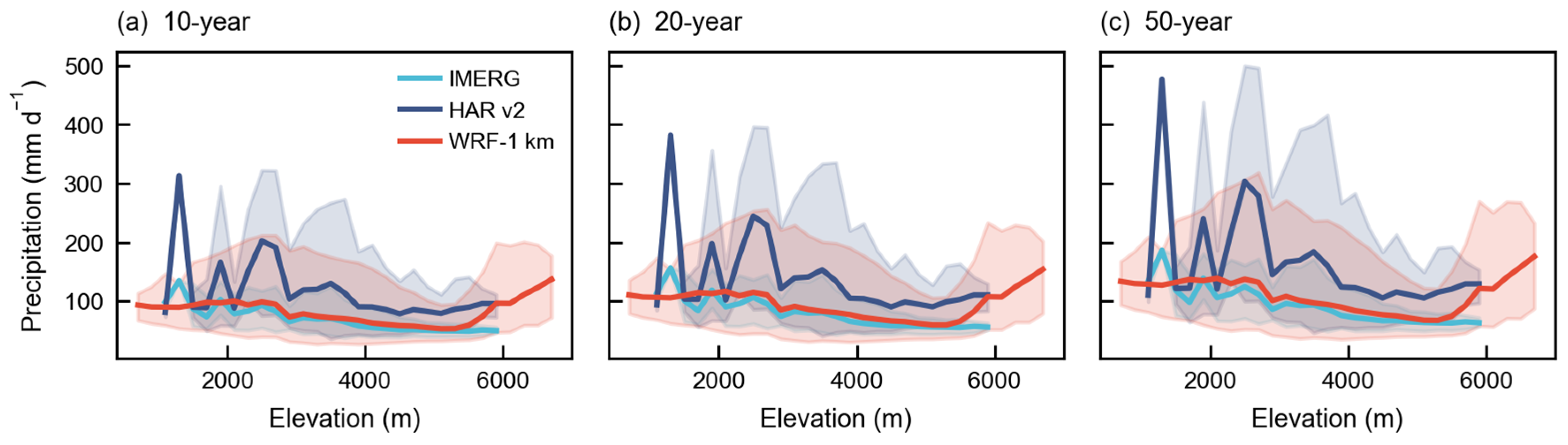
Figure 6 shows contrasting elevation dependencies of SMEV-derived precipitation extremes among the three datasets. The shaded envelope in each panel represents the 5th–95th percentile range of raw return-level values within each 200 m elevation bin, indicating data spread rather than a confidence interval of the mean. IMERG and HAR v2 both show return levels declining with elevation, steepening systematically above ~2700 m. The negative slopes intensify from the 10- to the 50-year return period: −9.07 to −13.28 mm d
−1 km
−1 (IMERG) and −18.20 to −28.80 mm d
−1 km
−1 (HAR v2). In both products, relationships at low elevations remain weak and statistically insignificant across all return periods. This likely reflects not only limited terrain sensitivity at a 10 km resolution, but also sparse sampling: the <2700 m zone contains only 55 grid cells (~5% of the 1150-cell domain) in each coarse dataset, so binned statistics in this range are subject to substantial sampling uncertainty.
By contrast, WRF-1 km exhibits a persistent three-phase elevation structure. At low elevations (600–2700 m, Phase I; 2628 cells, 2.8% of the domain), return levels increase with elevation for the 10-year return period (+4.53 mm d−1 km−1, p = 0.024), but the trend weakens progressively and becomes insignificant for the 50-year return period (+3.31 mm d−1 km−1, p = 0.14). Between 2700 and 5300 m (Phase II; 77,974 cells, 83.1% of the domain), return levels decrease sharply with elevation, with slopes steepening from −13.76 to −21.59 mm d−1 km−1 between the 10- and 50-year return periods (p < 0.001). This phase is constrained by the largest sample of any segment, giving high confidence in the moisture-starvation signal. Above ~5300 m (Phase III; 13,178 cells, 14.1% of the domain), the relationship reverses again, producing a strong positive trend that intensifies from +60.51 to +78.69 mm d−1 km−1 with increasing return period (R2 = 0.98, p < 0.001), corresponding to an approximately 2.3-fold increase in return levels between 5500 and 6700 m. We note that grid cells are unevenly distributed within Phase III: the 5300 m bin alone contains 8527 cells, whereas the two highest bins (6500–6700 m, n = 11–22) collectively contain only 33 cells. The standard error of the binned mean at elevations above 6300 m (5.6–16.7 mm d−1) is 3–10 times larger than at 5300–5900 m (0.3–3.9 mm d−1). The sign and statistical significance of the Phase III reversal are robust—the positive trend is consistently reproduced across all three return periods and is already established by the well-sampled bins at 5300–5900 m (>99% of Phase III cells). However, the precise slope magnitude carries greater uncertainty than the Phase II trend because the two highest bins, where the binned mean is least certain, exert leverage on the regression.
Across all three datasets, the steepening mid-elevation slopes point to moisture limitation that tightens with event rarity. The model-derived high-elevation reversal captured only by WRF-1 km reflects orographic forcing at the steepest ridges—a regime invisible to coarser products. The elevation dependence of precipitation extremes over SETP is therefore non-monotonic, with the governing physics shifting from moisture-limited decay at mid-elevations to mechanically forced intensification at the highest terrain.
5. Summary and Discussion
This study combined a 10-year convection-permitting WRF simulation at 1 km resolution with the SMEV framework to investigate precipitation extremes over SETP. Compared with the coarse-resolution IMERG and HAR v2 products, WRF-1 km substantially improves the representation of terrain-controlled extreme precipitation, resolving sharp windward–leeward contrasts and localized hotspots associated with the eastern Himalayas and the Tsangpo Grand Canyon. The results demonstrate that kilometer-scale convection-permitting simulations are essential for capturing the fine-scale spatial heterogeneity of precipitation extremes over complex mountain terrain.
Despite the relatively short simulation period, SMEV provides stable return-level estimates by exploiting a much larger sample of ordinary wet events than conventional annual-maximum approaches. At gauge locations, WRF-1 km reproduces observed return levels more accurately and with narrower uncertainty bounds than the coarse-resolution products, whereas IMERG and HAR v2 systematically overestimate long-return-period extremes because of intrinsic wet biases and artificially heavy distribution tails. The added value of the CPM becomes increasingly pronounced at longer return periods and higher elevations. Only WRF-1 km resolves localized extreme-value hotspots and reveals a non-monotonic elevation dependency characterized by moisture-limited decay at mid elevations and renewed intensification above ~5300 m associated with strong orographic uplift. These terrain-dependent structures are largely absent from the coarse-resolution datasets, even after statistical tail calibration. It should be noted that the intensification of precipitation extremes above 5300 m remains a model-derived phenomenon and lacks direct observational confirmation, owing to the absence of rain gauge measurements at such high elevations in the region.
Our finding that the 1-km CPM provides significant added value in resolving the spatial heterogeneity of extremes is consistent with the first ensemble of kilometer-scale simulations over the Third Pole. Similarly to those of Collier et al. (2024) [
19], our results demonstrate that explicitly resolving convection is crucial for capturing the correct magnitude of precipitation in complex terrain, where coarse-resolution products like IMERG and HAR v2 tend to overestimate mean maxima while smoothing out localized peaks. Despite this added value, the WRF-1 km simulation still exhibits a substantial error, which suggests that even at a 1 km resolution, the model may be unable to fully resolve microscale orographic features. Recent research emphasizes that at these resolutions, the impact of mesh size, turbulence parameterization, and land-surface-exchange schemes becomes critical for accurately simulating the mountain boundary layer and soil-atmosphere interactions [
37,
38]. These studies suggest that the remaining large errors in our 1 km simulation may have stemmed from unresolved micro-topography—such as gorges narrower than 1 km—or the sensitivity of the boundary layer schemes in such extreme terrain.
Several limitations nevertheless remain. First, the CPM record spans only ten years (2012–2021), and uncertainty in very long return periods (e.g., 100-year) remains unavoidable despite the use of the SMEV framework. However, the stationary assumption over a single decade is considered a reasonable compromise for high-resolution CPM studies, as computational costs often prohibit multi-decadal simulations at the kilometer scale. While SMEV provides more stable tail estimates than conventional annual-maximum methods by significantly increasing the effective sample size, these results should be interpreted as the current climatological potential of precipitation extremes as resolved by the 1 km CPM. Future research utilizing longer simulations, convection-permitting ensembles, or deep learning-based downscaling [
39] will be essential to further constrain these uncertainties and account for potential non-stationarity due to climate variability. Second, the systematic negative bias in annual maxima suggests that peak intensities may be underestimated at certain locations, potentially leading to non-conservative flood risk estimates if used directly without adjustment. Because rain gauges are concentrated in valley regions, the consistency of this bias across the topographic gradient (particularly above 5000 m) remains an open question. While we preserved the raw model output to highlight the added value of explicit convection and resolved topography, we recommend that practical applications in engineering and flood mitigation apply site-specific bias-correction techniques to ensure these CPM-SMEV estimates are anchored to local observational constraints. Third, a significant representativeness error exists because rain gauges are typically concentrated in valleys, which often receive less precipitation than the surrounding high-altitude ridges in the Tibetan Plateau. Comparing these point-based measurements to grid-cell averages in such extreme terrain inherently inflates the RMSE. To further investigate the physical drivers of these errors, we intend to compare our findings with recent international kilometer-scale ensembles—including those utilizing COSMO, ICON, and MPAS—that have been evaluated across the Third Pole [
19,
40].