Optimal Initial Error and Targeted Observation Sensitive Area for Predicting the Northeast China Cold Vortex Revealed by a Deep Learning Model

Abstract

The Northeast China Cold Vortex (NECV) is a key circulation system affecting weather patterns over North China, frequently triggering thunderstorms, hail, and other severe convective weather. Accurate prediction of NECVs is therefore of great importance. However, substantial forecast errors still remain, largely due to uncertainties in the initial conditions. To improve NECV forecast skills, we investigate the optimal initial errors and targeted observation sensitive areas using a sampling-based approximation of the conditional nonlinear optimal perturbation (CNOP) method together with the Pangu-Weather deep learning model. We first evaluate the model’s performance over Northeast China and find that Pangu-Weather exhibits forecast skill generally comparable to the ECMWF Integrated Forecasting System (IFS) during the May–August 2022 period over Northeast China. Then the CNOP-based approach is used to capture the optimal initial errors with the greatest impact on NECV forecasts. The largest error amplitudes are primarily located upstream of the vortex and near upper-level jet-entrance regions, which are identified as the targeted observation sensitive areas. Perturbation kinetic-energy diagnostics further indicate that baroclinic conversion is the dominant mechanism for error growth. Observing system simulation experiments suggest that, under an idealized assumption of completely eliminating errors in a given region, targeted observations over the sensitive area can produce the largest forecast improvement, with an average error reduction of approximately 13% relative to other areas. This study contributes to a deeper understanding of NECV predictability and may help improve forecasting capability.

1. Introduction

The Northeast China Cold Vortex (NECV) is a cut-off low system that frequently occurs over East Asia [1,2]. During the boreal summer, prevailing northerly flow over the mid-to-high latitudes favors the formation and maintenance of NECVs, leading to a substantial increase in their frequency [3,4]. NECVs are characterized by cold lows in the mid-to-upper troposphere, marked by frequent generation, slow movement, and intense convective activity [5]. Associated severe weather—including heavy rainfall, thunderstorm winds, hail, and summer cold damage—seriously threatens regional socio-economic activities and agricultural production [5,6]. Enhancing NECV predictability is, therefore, essential for climate security and disaster mitigation in northern China.

NECV forecasting has traditionally relied on numerical models, which integrate atmospheric dynamical and thermodynamical equations based on specified initial and boundary conditions [7,8,9]. Major operational centers such as the European Centre for Medium-Range Weather Forecasts (ECMWF) [10] and the National Centers for Environmental Prediction (NCEP) have established high-resolution global models capable of capturing mid-latitude systems. However, forecast accuracy remains constrained by initial errors, which are often amplified by observational limitations, data assimilation uncertainties, and atmospheric nonlinearity [11,12,13]. Furthermore, this challenge is particularly acute for rapidly evolving, structurally complex mesoscale systems such as NECVs [14].

Rapid advances in deep learning have opened new avenues for weather and climate prediction [9,15,16,17]. By leveraging large-scale datasets, deep learning models can directly learn nonlinear atmospheric evolution from reanalysis data and observations, bypassing the need for explicit dynamical equations [18,19,20]. Notably, the Pangu-Weather model [21] has demonstrated forecast performance comparable to, or even surpassing, that of the ECMWF Integrated Forecasting System (IFS), while drastically reducing computational costs. However, similar to traditional numerical models, deep learning forecasts are also sensitive to initial-condition errors [20].

To mitigate the limitations imposed by initial-error growth, previous studies introduced the concept of targeted observations [22,23], in which additional observations were deployed in the most sensitive regions to maximize forecast accuracy at the target time. Common sensitive-area identification methods include ensemble Kalman filter [12,24], singular vectors [25,26], and conditional nonlinear optimal perturbation (CNOP) [27,28,29]. The former two methods rely on linear approximations and therefore have limitations in representing nonlinear error growth. In contrast, the latter method is fully nonlinear and can effectively capture the optimal initial error, i.e., the initial perturbation that produces the largest forecast-error growth under a prescribed constraint, thereby efficiently identifying targeted observation sensitive areas.

Traditional targeted observation studies mainly rely on numerical weather prediction models, where repeated integrations for sensitivity analysis are computationally expensive. In contrast, deep-learning weather models such as Pangu-Weather provide substantially faster forecast inference. Compared with traditional numerical weather prediction (NWP) integrations that may require minutes to hours per forecast cycle, Pangu-Weather completes inference within seconds, enabling hundreds of perturbation experiments at feasible cost. This computational advantage makes large-sample sensitivity experiments feasible. Therefore, integrating the CNOP framework with a deep-learning forecasting model provides an efficient framework for predictability diagnosis and targeted observation design. In this study, we identify the optimal initial errors and targeted observation sensitive areas using the Pangu-Weather model and a CNOP-based approach, and then employ observing system simulation experiments (OSSEs) to evaluate the effectiveness of reducing errors in sensitive regions for improving forecast accuracy.

The remainder of this paper is organized as follows. Section 2 introduces the datasets and methods. Section 3 evaluates model forecast performance, identifies the fastest-growing (optimal) initial errors, examines the physical mechanisms of the error growth, and finally assesses targeted observation sensitive areas through OSSEs. Section 4 summarizes the main findings and discusses the methodological implications and limitations of this study.

2. Materials and Methods

2.1. Data

This study primarily utilizes data from the ECMWF Fifth Generation Global Atmospheric Reanalysis product (ERA5; [30]). Operated by ECMWF on behalf of the Copernicus Climate Change Service (C3S), ERA5 integrates multi-source historical observations (including satellite, radar, radiosonde, aircraft, and surface stations) into a consistent global climate estimate using four-dimensional variational data assimilation (4D-Var) and an advanced model system, with time coverage extending from 1940 to the present.

ERA5 provides an extensive suite of atmospheric, land-surface, and oceanic variables at an hourly resolution. The vertical structure is represented by 137 model levels extending from the surface to approximately 80 km, with standard pressure-level products covering 37 isobaric heights. To meet the input requirements of the Pangu-Weather model, we extract key meteorological variables for the period of May–August 2022. The three-dimensional atmospheric field is constructed using five upper-air variables—geopotential height, specific humidity, temperature, and U/V wind components—across 13 mandatory pressure levels. Additionally, four surface variables—mean sea-level pressure, 10 m U/V wind components, and 2 m temperature—are selected. All ERA5 data are processed on a uniform 0.25° × 0.25° grid to align with the input resolution of Pangu-Weather model.

To evaluate the deep learning model’s performance against traditional numerical methods, the forecast products from the ECMWF-IFS are employed as a baseline. To ensure a rigorous and fair comparison, the ECMWF-IFS data are selected for the same variables, time periods, and spatial resolution (0.25° × 0.25°) as the ERA5-driven Pangu-Weather forecasts.

2.2. Pangu-Weather Deep Learning Model

Pangu-Weather is a global deep-learning weather forecasting model developed by the Huawei Cloud team [21]. Trained on ERA5 reanalysis data, the model features a specialized framework tailored to the three-dimensional structure of the atmosphere. This is achieved through a 3D block strategy, local 3D self-attention, and relative position encoding adapted to the Earth’s spherical geometry, enabling end-to-end modeling of complex atmospheric spatiotemporal evolution. Based on a single initial state, Pangu-Weather outputs key meteorological variables—including temperature, wind fields, geopotential height, and specific humidity—across multiple vertical levels covering the troposphere. The model provides a global uniform grid resolution of 0.25° × 0.25°, with a forecast lead time extending to approximately 10 days. Its medium-range performance has been shown to be comparable to, or even surpass, traditional numerical models across various evaluation metrics.

During inference, Pangu-Weather bypasses the step-by-step integration of dynamical and physical processes used in traditional NWP models. Instead, it predicts the atmospheric 3D state at subsequent intervals via a single forward pass through the deep learning network. This study utilizes the publicly available 24 h time-step model, where each forward calculation yields a forecast for the following 24 h. This strategy minimizes the number of iterative steps required for multi-day forecasts, significantly reducing cumulative errors and computational overheads.

2.3. Study Area and Case Selection

The model evaluation domain in this study is defined as 110°–145° E and 35°–60° N, corresponding to the NECV activity region [31]. Within this broader domain, Liu et al. [32] identified 120°–130° E and 40°–50° N as the key region for NECV, where variations in 500-hPa geopotential height effectively characterize the system’s life cycle. Accordingly, the regional mean geopotential height within this key region is used to define the NECV Activity Index (NECVI). Three typical NECV cases that occurred between May and August 2022 are selected for analysis (Cases 1–3). The mature stages of these cases are 7–9 May, 26–28 May, and 8–10 July 2022, respectively.

2.4. Identification of the Optimal Initial Error Using the CNOP Approach

To capture the optimal initial error (the fastest-growing initial error), we employ the CNOP approach proposed by Mu et al. [27]. For simplicity, the CNOP-type optimal initial errors are obtained by the re-forecast experiments, following Feng and Duan [33]. This sampling-based strategy provides a practical approximation of the CNOP. It effectively identifies perturbations with the largest nonlinear growth under the prescribed constraints. Previous predictability studies have shown that this approach can capture robust sensitive-error structures [33,34]. The experimental domain spans 80°–150° E and 10°–80° N, covering the main circulation systems of the mid-to-high latitudes and the evolution of NECVs.

The specific experimental procedure is as follows. First, after determining the initial forecast time, two datasets within a three-month period and separated by 3–5 days are randomly selected. Differences in temperature, zonal wind, and meridional wind at the surface and across 13 upper-air pressure levels are then calculated. These differences are scaled to 0.3 times their standard deviation, serving as a physical constraint for constructing a random initial error field. The imposed perturbation amplitude (0.3 σ) represents a moderate perturbation amplitude. Comparison with the calculated perturbation magnitudes indicates that they are broadly comparable to typical observational uncertainty ranges for atmospheric temperature and wind. The resulting perturbation is then superimposed onto the original model input, and Pangu-Weather is used to perform 5-day forecasts. The above procedure is repeated 500 times.

To quantify the impact of initial errors on forecast results, the dry energy of the forecast error is calculated over the region where NECVs frequently occur. The forecast error is defined as the difference between the perturbed forecast and the control forecast (i.e., the forecast without superimposed perturbations). This metric characterizes the temporal evolution of dry-energy error growth at different forecast lead times. The dry-energy norm (E) of the error is defined as:

$$\mathrm{E} = {\displaystyle \frac{1}{{\mathrm{D}}_1}}{\int }_{{\mathrm{D}}_1}{\int }_0^1[{\mathrm{u}\prime }^2 + {\mathrm{v}\prime }^2 + {\displaystyle \frac{{\mathrm{c}}_{\mathrm{p}}}{{\mathrm{T}}_{\mathrm{r}}}}{\mathrm{T}\prime }^2 + {\mathrm{R}}_{\mathrm{a}}{\mathrm{T}}_{\mathrm{r}}{\left({\displaystyle \frac{{\mathrm{p}}_{\mathrm{s}}^{\prime }}{{\mathrm{p}}_{\mathrm{r}}}}\right)}^2]\mathrm{d}\mathsf{\sigma }\mathrm{d}{\mathrm{D}}_1,$$

(1)

In this equation, the dry-energy error $E$ consists of kinetic-energy and effective potential-energy components. The zonal and meridional wind errors ($\mathrm{u}\prime$ and $\mathrm{v}\prime$) represent the kinetic-energy contribution associated with wind-field perturbations, while the temperature and surface-pressure error terms ($\mathrm{T}\prime$ and ${\mathrm{p}}_{\mathrm{s}}^{\prime }$) describe the effective potential-energy contribution associated with thermal and mass-field anomalies. Here, ${\mathrm{R}}_{\mathrm{a}}$ is the gas constant for dry air, with a value of 287 J kg⁻¹K⁻¹. ${\mathrm{T}}_{\mathrm{r}}$ is the reference temperature, and ${\mathrm{c}}_{\mathrm{p}}$ is the specific heat at constant pressure.

We first calculate the squared error terms of the key variables over region ${\mathrm{D}}_1$ and perform area averaging. Next, mass integration is carried out in the vertical $\mathsf{\sigma }$ coordinates. This procedure yields a scalar value $\mathrm{E}$, which represents the vertically integrated, mass-weighted dry-energy error per unit mass within the target region ${\mathrm{D}}_1$. Physically, $\mathrm{E}$ corresponds to the sum of the kinetic energy and effective potential energy of the error. Because NECV evolution involves coupled thermodynamic and dynamical processes, the dry-energy norm is suitable for measuring forecast-error growth associated with NECV development.

Based on the above re-forecast experiments, the 20 perturbations with the most pronounced dry-energy growth at the 5-day lead time are selected. These 20 “rapid-growth initial-error” fields are regarded as the optimal initial error. Their spatial structures are used to identify the targeted observation sensitive regions for improving the prediction of the NECV.

2.5. Perturbation Kinetic-Energy Budget Analysis

To reveal the energy sources and conversion mechanisms during the growth of initial errors (perturbations), a perturbation kinetic-energy budget equation is employed for diagnostic analysis. All variables are defined as differences between the perturbed experiment and the reference state.

2.5.1. Definition of Perturbation Kinetic Energy

The perturbation kinetic energy is defined as the kinetic energy associated with wind-field errors:

$$\mathrm{K} = {\displaystyle \frac{1}{2}}(\mathrm{u}{\prime }^2+\mathrm{v}{\prime }^2),$$

(2)

where u′ and v′ denote the zonal and meridional wind error components, respectively.

2.5.2. Perturbation Kinetic-Energy Budget Equation

The temporal tendency of perturbation kinetic energy can be decomposed into barotropic conversion, baroclinic conversion, and advection terms:

$${\displaystyle \frac{\partial \mathrm{K}}{\partial \mathrm{t}}} ={ \mathrm{C}}_{\mathrm{BT} }+ {\mathrm{C}}_{\mathrm{BC}} +{ \mathrm{C}}_{\mathrm{ADV}},$$

(3)

where ${\mathrm{C}}_{\mathrm{BT}}$ is the barotropic conversion term, ${\mathrm{C}}_{\mathrm{BC}}$ is the baroclinic conversion term, and ${\mathrm{C}}_{\mathrm{ADV}}$ is the advection term.

• Barotropic Conversion Term (BT)

Barotropic conversion represents the momentum exchange between the mean flow and perturbation kinetic energy:

$${\mathrm{C}}_{\mathrm{BT}} = -\mathrm{u}{\prime }^2{\displaystyle \frac{\partial \mathrm{U}}{\partial \mathrm{x}}} - \mathrm{u}\prime \mathrm{v}\prime {\displaystyle \frac{\partial \mathrm{U}}{\partial \mathrm{y}}} - \mathrm{u}\prime \mathrm{v}\prime {\displaystyle \frac{\partial \mathrm{V}}{\partial \mathrm{x}}} - \mathrm{v}{\prime }^2{\displaystyle \frac{\partial \mathrm{V}}{\partial \mathrm{y}}},$$

(4)

where U and V are the zonal and meridional components of the reference-state wind field.

• Baroclinic Conversion Term (BC)

Baroclinic conversion describes the conversion of available potential energy into kinetic energy:

$${\mathrm{C}}_{\mathrm{BC}} = \mathrm{g}{\displaystyle \frac{\mathrm{w}\prime \mathrm{T}\prime }{\mathrm{T}}},$$

(5)

where w′ is the perturbation vertical velocity, T′ is the perturbation temperature, and T is the reference-state temperature.

It should be noted that Pangu-Weather does not explicitly output some variables, such as vertical velocity. Therefore, the ${\mathrm{C}}_{\mathrm{BC}}$ term in the budget analysis is estimated approximately using the mass continuity equation, which may introduce some uncertainty into the quantitative results. Nevertheless, this method can still capture the primary energy-conversion pathways during perturbation growth and provides useful insight into the mechanisms of forecast-error amplification.

• Advection Term (ADV)

The advection term represents the transport of perturbation kinetic energy by the reference-state flow, including both horizontal and vertical advection:

$${\mathrm{C}}_{\mathrm{ADV} }= -\mathrm{U}{\displaystyle \frac{\partial \mathrm{K}}{\partial \mathrm{x}}} - \mathrm{V}{\displaystyle \frac{\partial \mathrm{K}}{\partial \mathrm{y}}} - \mathrm{W}{\displaystyle \frac{\partial \mathrm{K}}{\partial \mathrm{z}}},$$

(6)

Because the model output does not provide sufficient diagnostic variables to accurately quantify subgrid-scale and frictional processes, the dissipation term is not explicitly calculated in this study.

3. Results

3.1. Evaluation of Pangu-Weather’s Performance in Predicting NECV

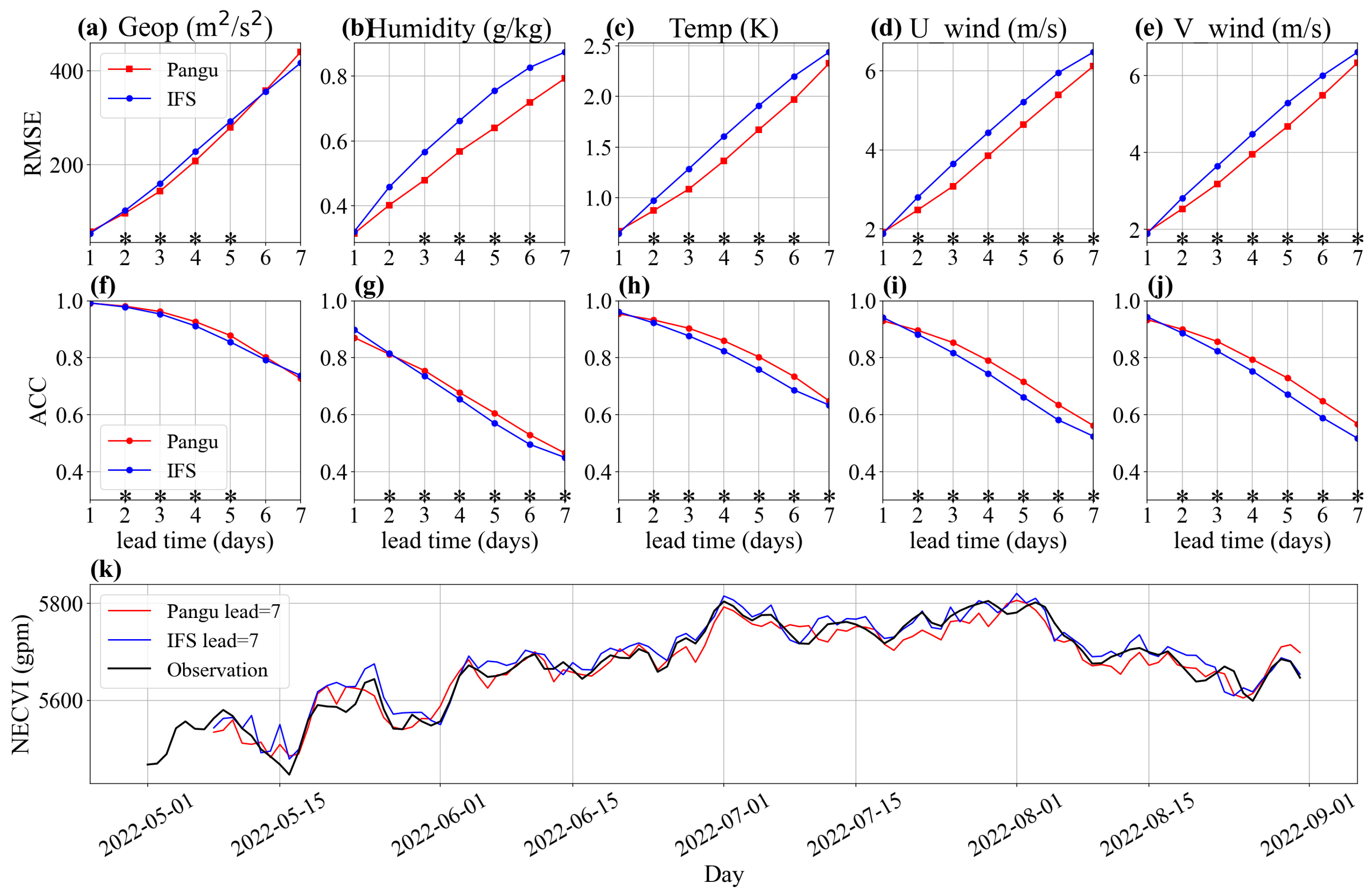
To evaluate the forecasting capabilities of Pangu-Weather in the Northeast China region, we compare its predictions and those of ECMWF-IFS, including the key atmospheric circulation variables during the period of May–August 2022. Figure 1 shows the root-mean-square error (RMSE) and anomaly correlation coefficient (ACC) calculated from forecasts by the Pangu and IFS models, alongside the observational data. The results imply that for 1–7-day forecasts of geopotential height, specific humidity, temperature, and wind field, Pangu-Weather generally yields comparable or slightly lower RMSE than ECMWF-IFS. Although this improvement is evident across all parameters, there are inter-variable variations: the reductions in RMSE for temperature and humidity are more substantial, whereas the improvement for geopotential height is relatively modest. Consistent with the RMSE results, the ACC metrics reveal a modest advantage for the deep learning model; Pangu-Weather maintains higher ACC scores than the IFS for nearly all variables throughout the 7-day forecast period. From Figure 1k, we can also see that the predicted NECVIs of the Pangu-Weather model and IFS model are very close to the observed index.

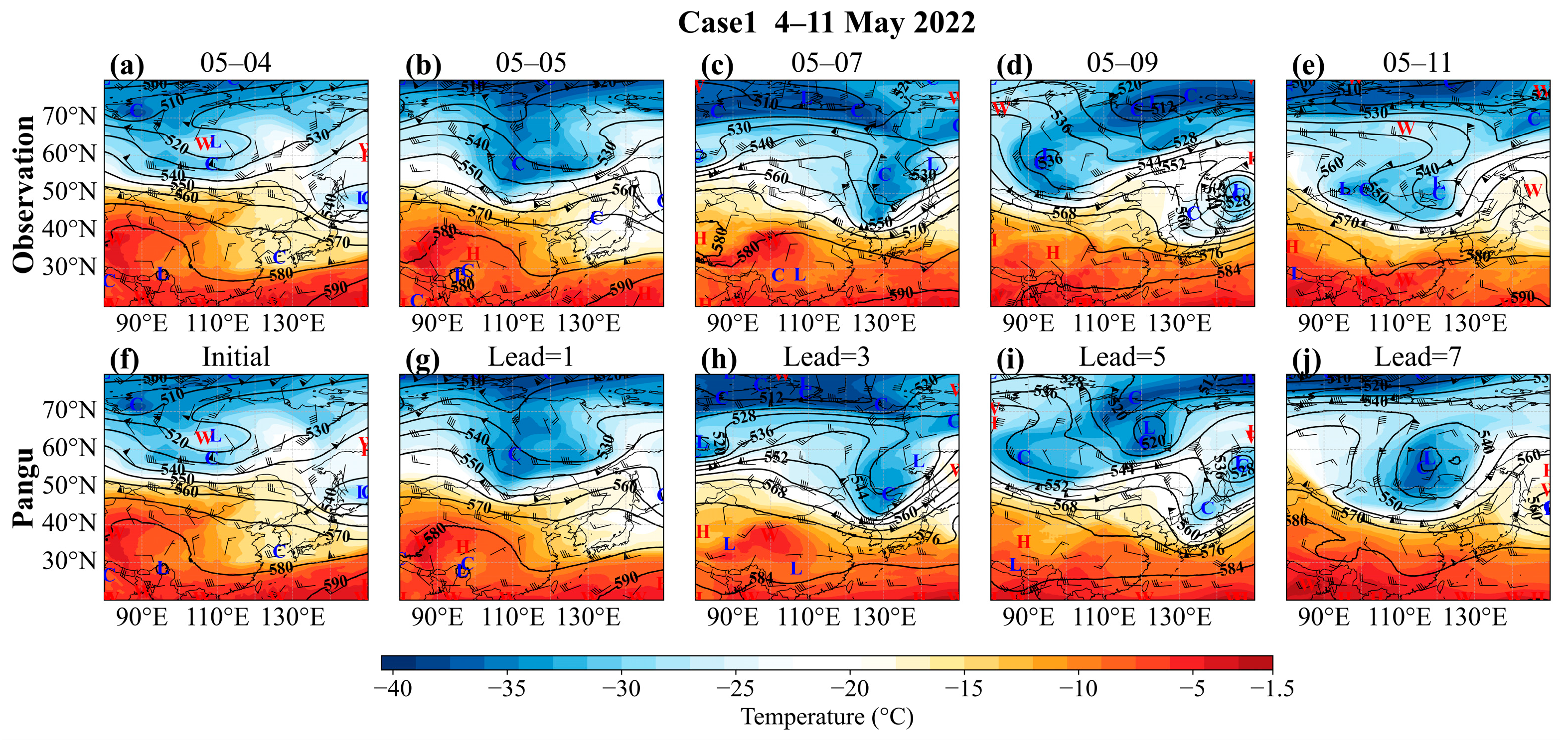
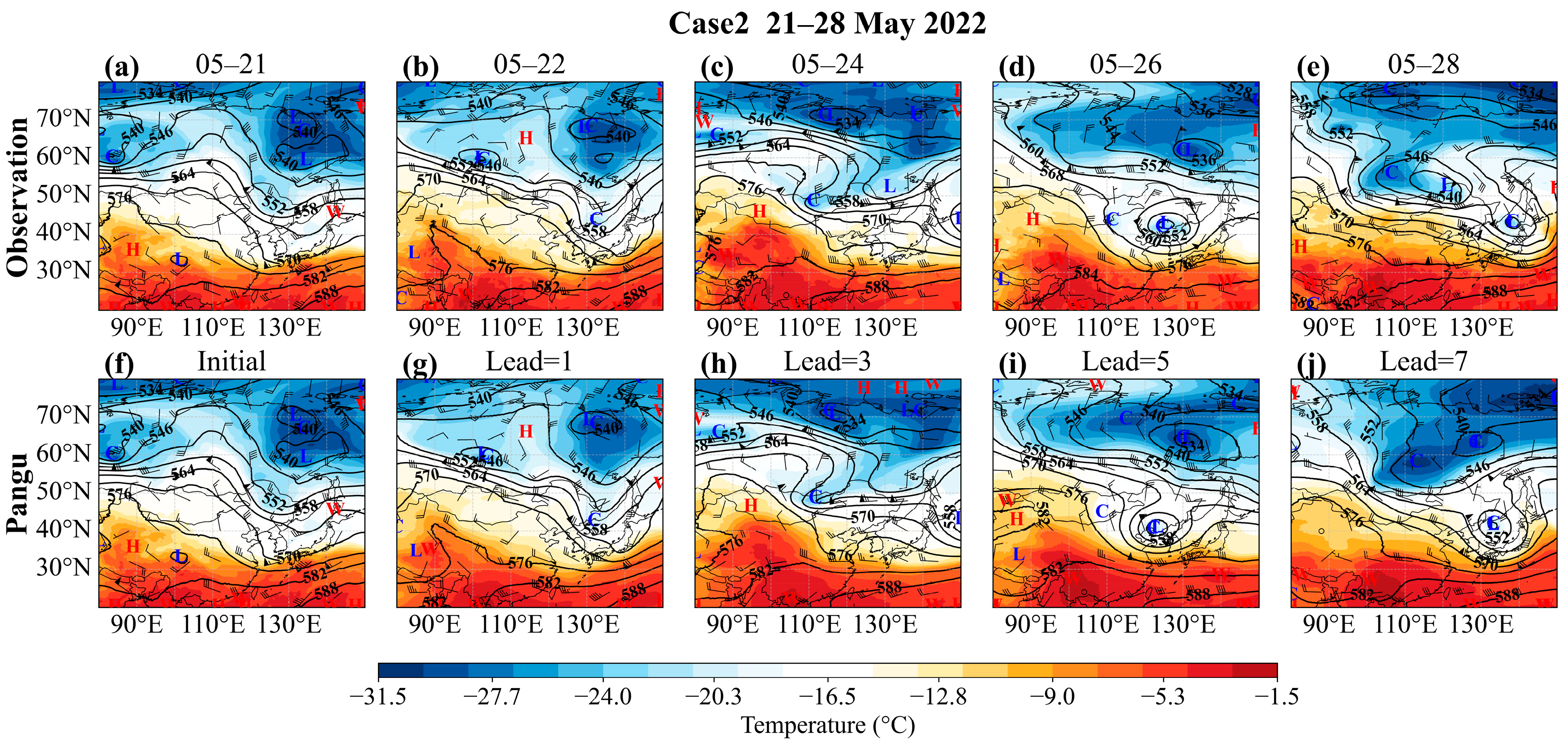
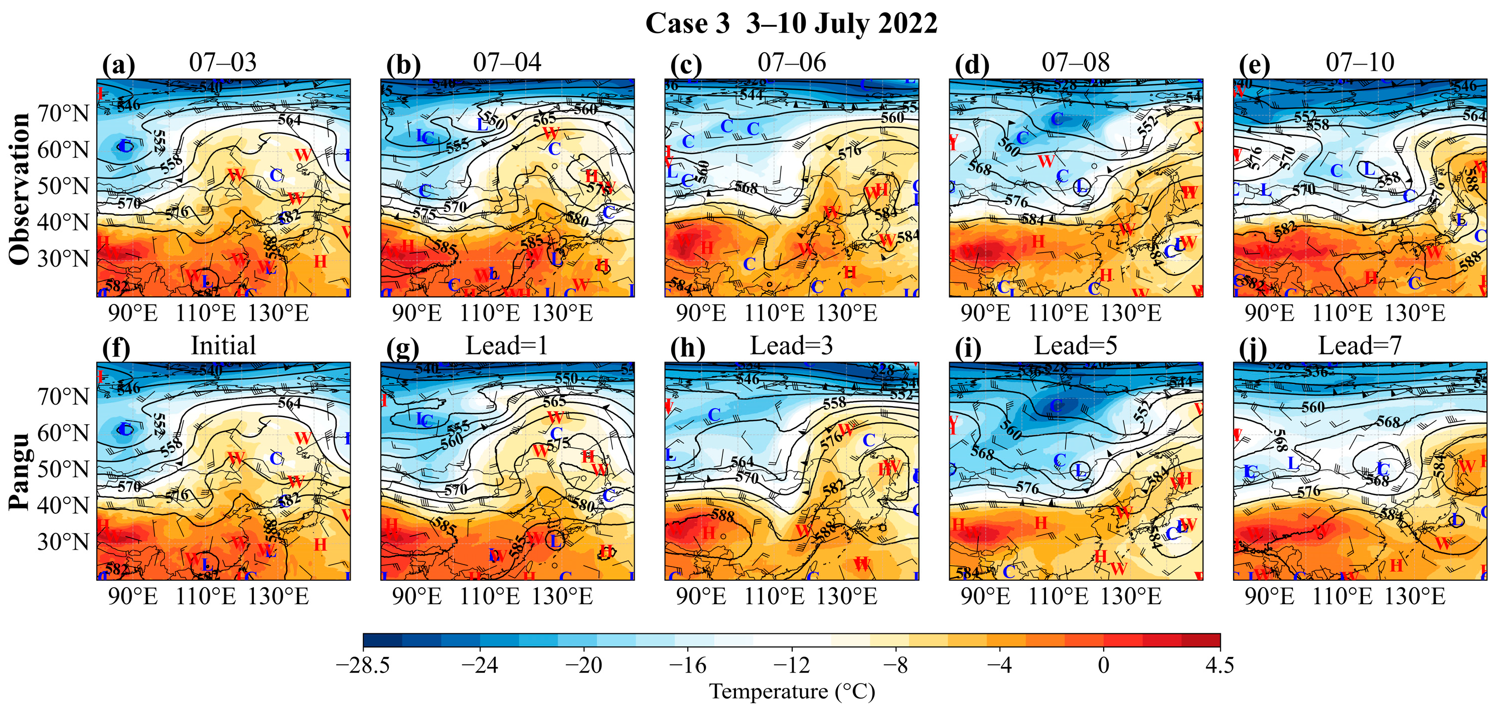
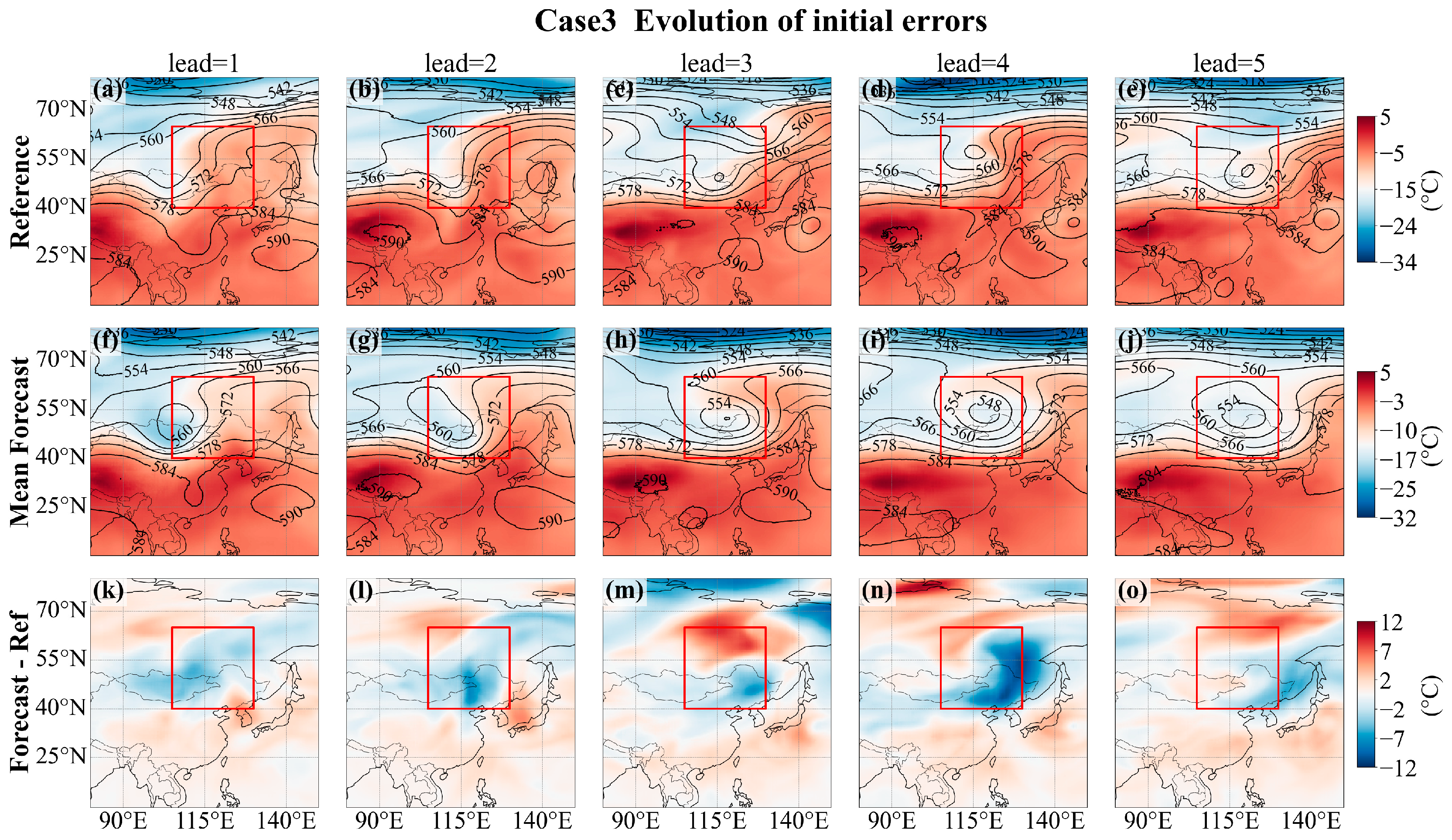
To further evaluate the capability of Pangu-Weather in predicting the NECV, three representative cases are analyzed: Case 1 (7–9 May), Case 2 (26–28 May), and Case 3 (8–10 July). Figure 2, Figure 3 and Figure 4 compare the observed 500-hPa temperature fields (shading) and geopotential height fields (black contours) with Pangu-Weather forecasts at various lead times.

Pangu-Weather reproduces the main structural characteristics of the cold vortex, including its location, morphology, and intensity, and maintains reasonable forecast skill for both quasi-stationary and rapidly evolving NECV cases up to a 7-day lead time. These results support the use of Pangu-Weather in the subsequent sensitivity experiments.

3.2. Optimal Initial Errors in the NECV Prediction Based on Pangu-Weather Model

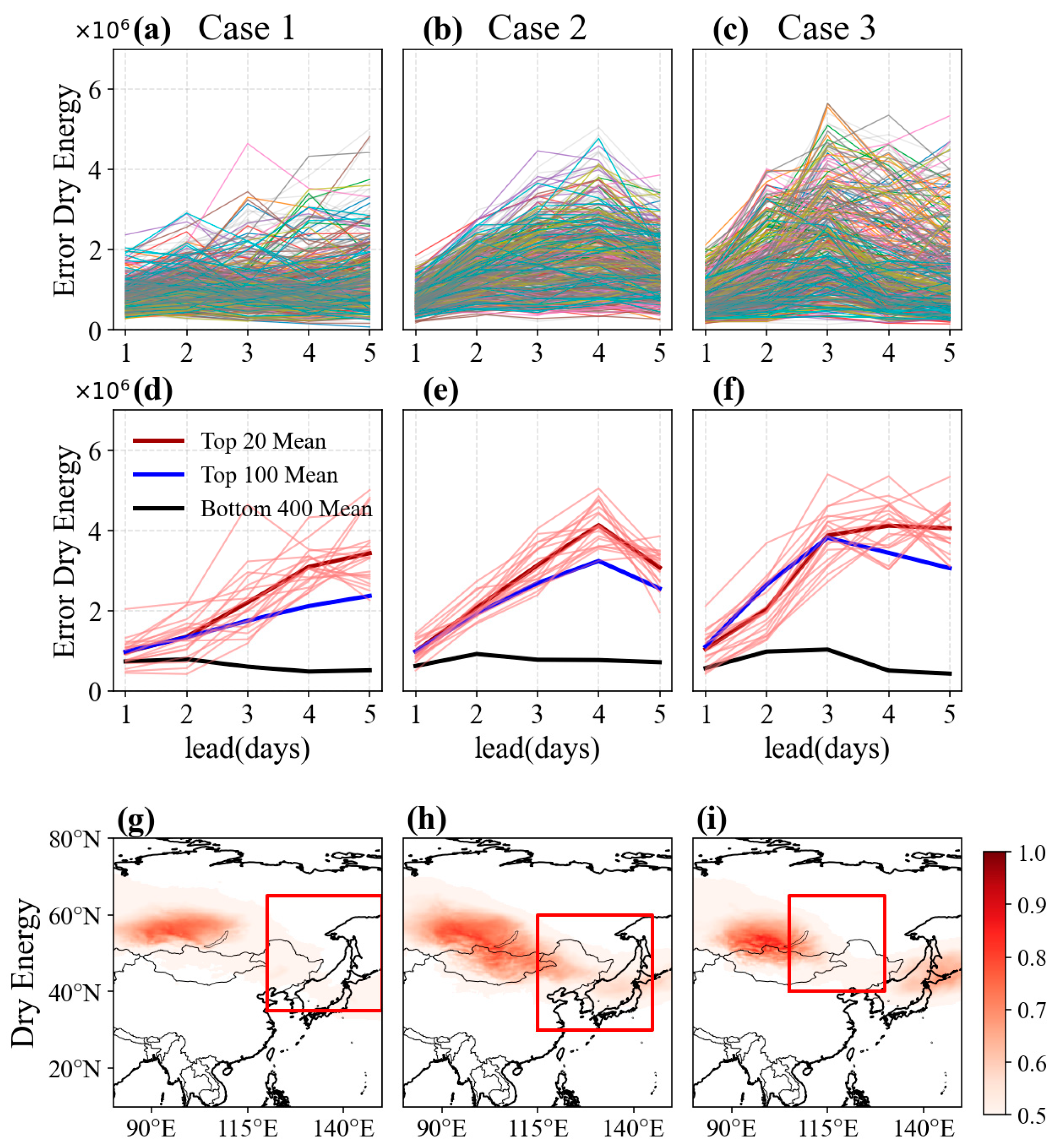
Figure 5 illustrates the energy evolutions of the initial errors for three representative NECV cases. By computing the dry-energy norm of forecast errors within the primary NECV activity region (indicated by the red box), the growth trajectories of the initial-error energy are obtained. Overall (Figure 5a–c), a subset of initial errors exhibits rapid amplification, reaching peak magnitudes around forecast Days 2–3, a clear manifestation of nonlinear error growth. In contrast, the remaining errors show relatively limited growth. We further isolate the 20 initial errors with the most pronounced energy growth at the 5-day lead time (Figure 5d–f). These optimal initial errors exhibit a consistent evolution process, characterized by an initial stage of rapid intensification followed by a gradual saturation phase as the forecast lead time increases.

For comparison, the mean evolutions of the top 100 and bottom 400 perturbation groups are also shown. The top 100 group displays a growth pattern broadly similar to that of the top 20 group, although with weaker amplitudes, whereas the bottom 400 group remains nearly unchanged throughout the forecast period. This contrast suggests that the rapidly growing perturbations may share similar error-growth characteristics, and that the selected top 20 subset provides a useful approximation of the fastest-growing perturbations.

Subsequently, a composite analysis of these 20 optimal initial errors is conducted to identify their spatial structures. The results reveal prominent localized distribution characteristics (Figure 5g–i), with initial-error maxima primarily concentrated over Northeast China, the Mongolian Plateau, and the region south of Lake Baikal. These results suggest that NECV forecast errors may be influenced by initial-field uncertainties in these upstream regions.

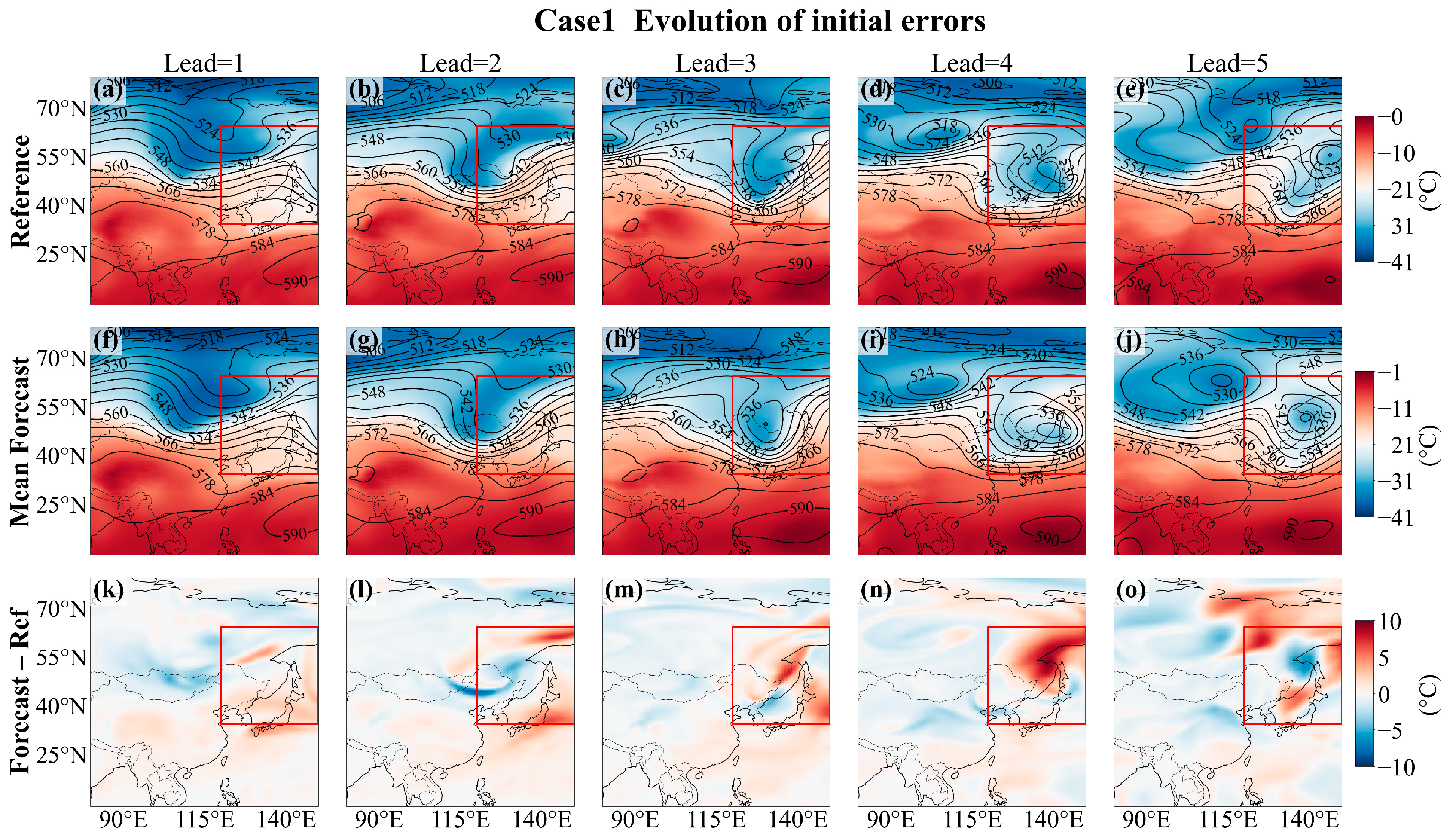
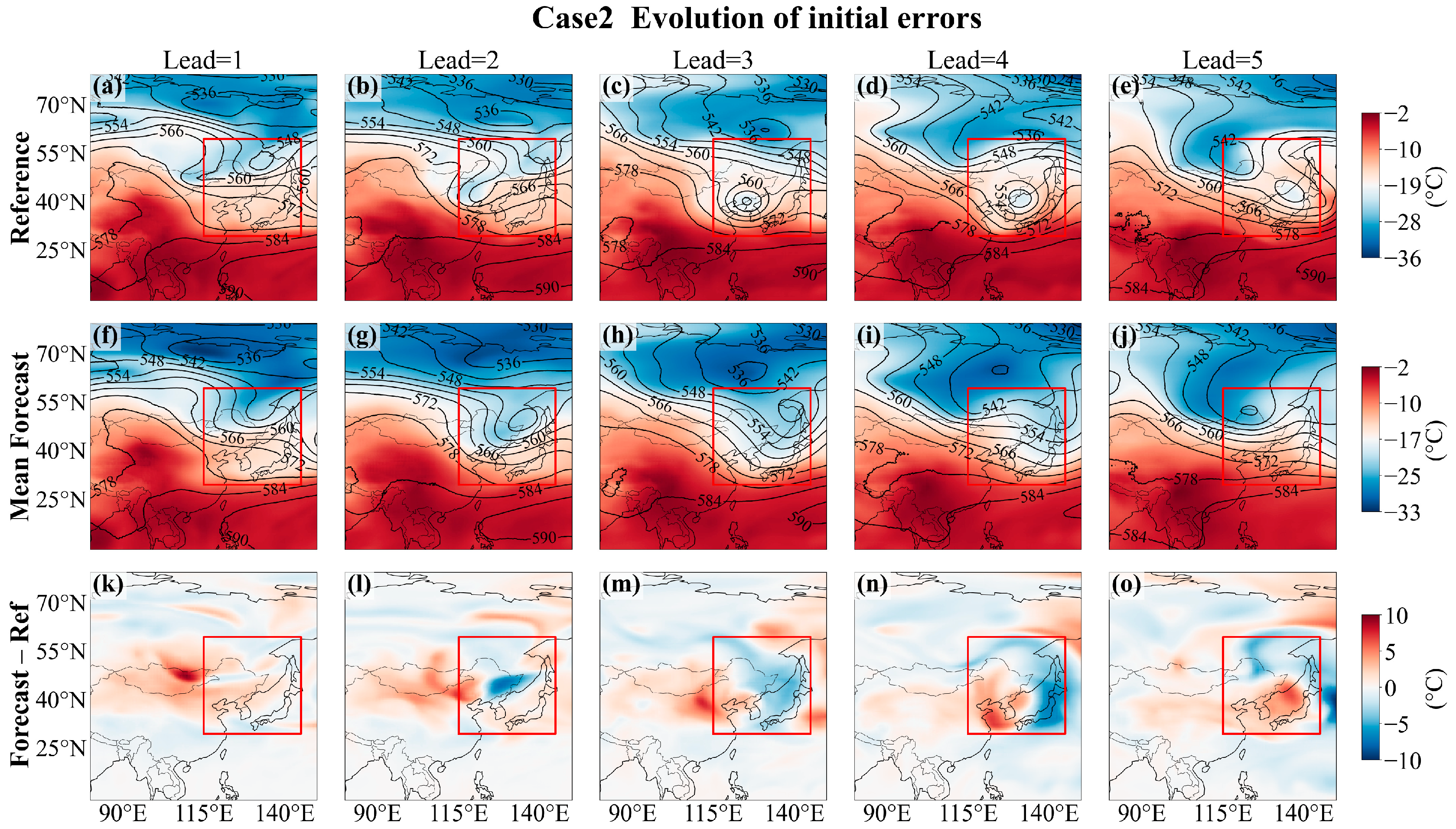
To evaluate the impact of the optimal initial errors on NECV predictability, sensitivity experiments are conducted within the Pangu-Weather model. For each case, the temporal evolution of the 20 initial perturbations exhibiting the most pronounced energy growth is composited. Figure 6, Figure 7 and Figure 8 show the control forecasts, the corresponding composite perturbed forecasts, and their difference fields for the 500-hPa atmospheric state.

Overall, the optimal initial errors are associated with substantial changes in the forecast evolution and intensity of the cold vortex. For Cases 1 and 3, the composite perturbed forecasts (Figure 6 and Figure 8) exhibit deeper geopotential height contours and enhanced temperature gradients, suggesting a more intense cold trough that deepens and propagates downstream. These features indicate that the identified optimal initial errors tend to amplify the cold-vortex system in these cases. In contrast, for Case 2 (Figure 7), the perturbed geopotential height field becomes shallower and the cold core weakens. This response suggests that the initial errors act to suppress the cold-vortex structure, consistent with the eastward propagation and decay stage of this case.

Despite these contrasting intensity responses, a coherent spatiotemporal pattern of error growth is evident across all three cases. Forecast errors initially concentrate near the frontal zone ahead of the developing cold trough, and subsequently amplify rapidly along the westerly jet before propagating downstream. This evolution follows a characteristic pattern of localized perturbation amplification followed by downstream development [35]. Throughout this process, the error fields are advected by the background wind while maintaining a high degree of spatial coherence. These results suggest that the identified optimal initial-error structures can promote nonlinear error growth in Pangu-Weather and subsequently affect NECV forecasts.

3.3. The Development Mechanism of the Optimal Initial Error

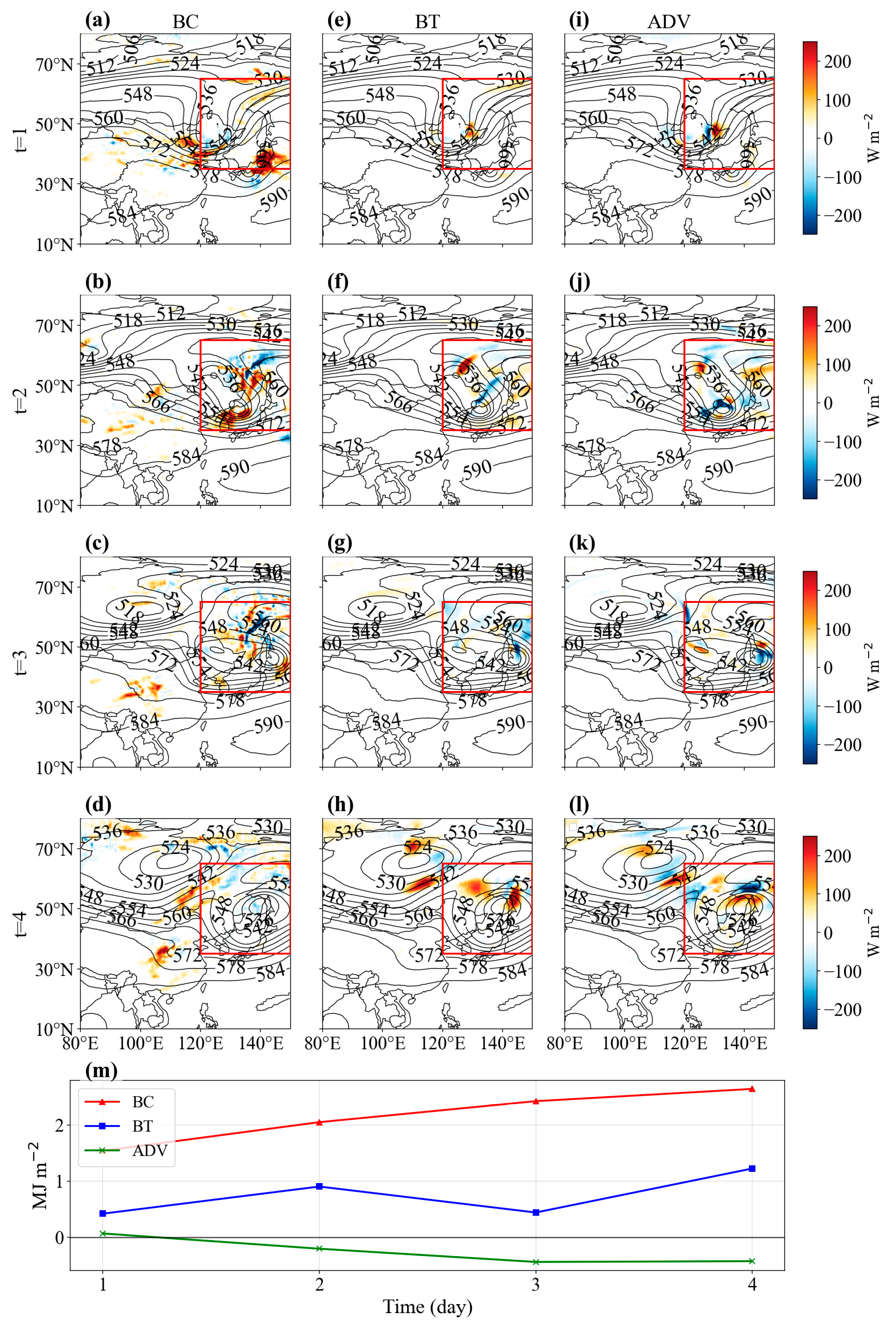
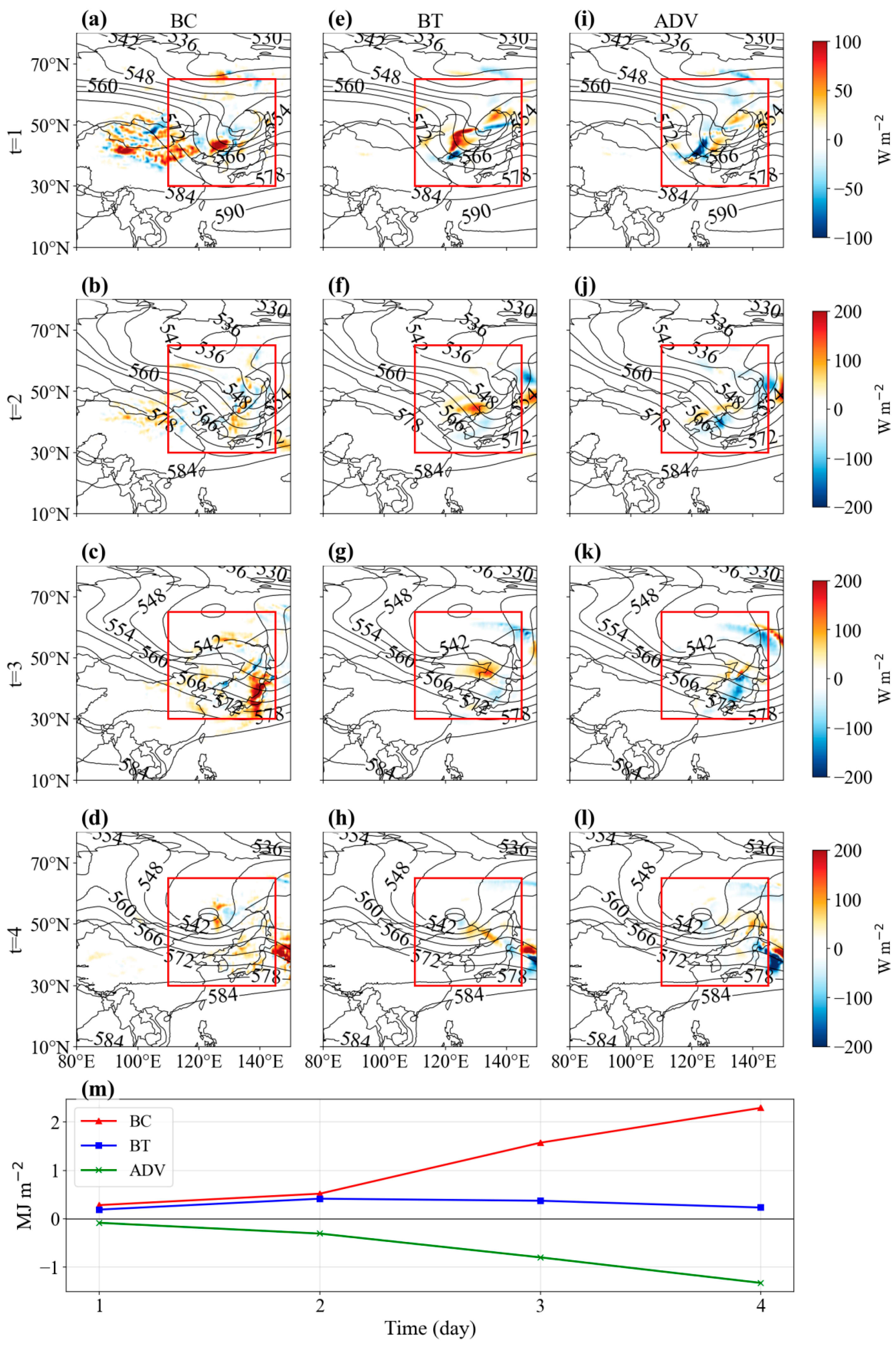
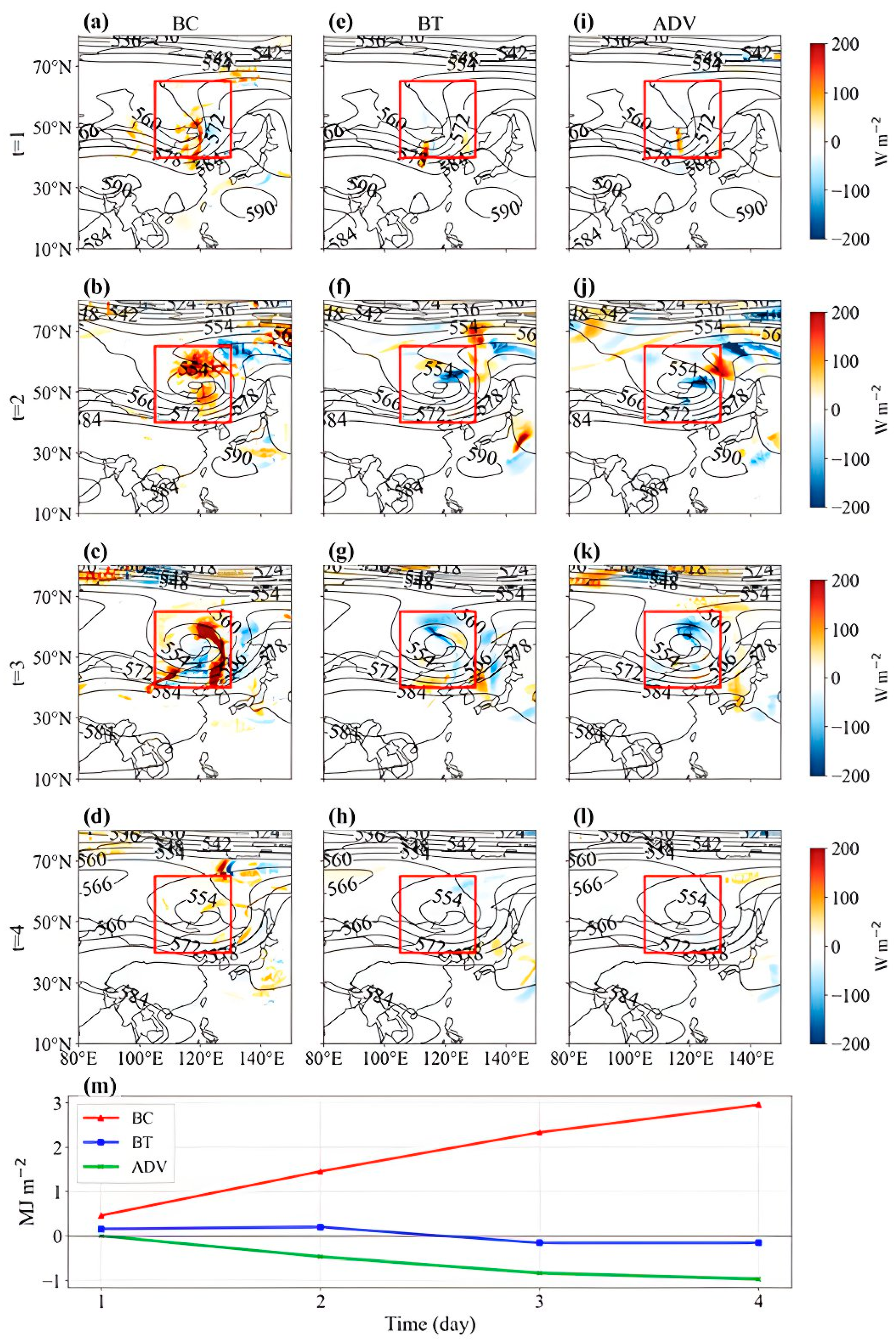
To further understand the energy-evolution mechanisms during the error growth, this subsection examines the perturbation kinetic-energy budget (see Section 2.5), focusing on the contributions of BC, BT, and ADV, as shown in Figure 9, Figure 10 and Figure 11. The time series (panel m in each figure) show a consistent feature among the three cases: BC is the dominant source of perturbation kinetic-energy growth, whereas BT and ADV play comparatively secondary roles.

In Case 1, perturbation kinetic-energy growth is mainly driven by BC, which gradually intensifies and reaches its maximum during the later stage, indicating continuous conversion of mean-flow available potential energy into kinetic energy. BT remains weak, and ADV stays close to zero, suggesting limited contributions from momentum transport and advection. Spatially, strong BC is concentrated ahead of the trough and near the warm sector, consistent with regions of strong temperature gradients.

Case 2 exhibits a similar structure, with BC still dominating the growth process. BT shows only weak positive contributions in the early stage. In contrast to Case 1, ADV becomes increasingly negative, implying that advection suppresses system development through outward energy transport, mainly in the downstream region.

Case 3 shows the strongest baroclinic signature. BC increases continuously and more strongly than in the other two cases, indicating more efficient energy extraction from the background field. BT remains weak and becomes slightly negative in the later stage, while ADV also shows persistent negative contributions, suggesting clear outward energy dispersion.

Overall, the three cases suggest that baroclinic conversion is the primary mechanism for perturbation kinetic-energy growth, whereas barotropic conversion is generally weak and advection may suppress development in some cases. These results suggest that baroclinic instability likely plays a major role in NECV evolution, while initial errors modulate system intensity and structure by influencing the energy-conversion processes.

3.4. Identification of the Targeted Observation Sensitive Areas

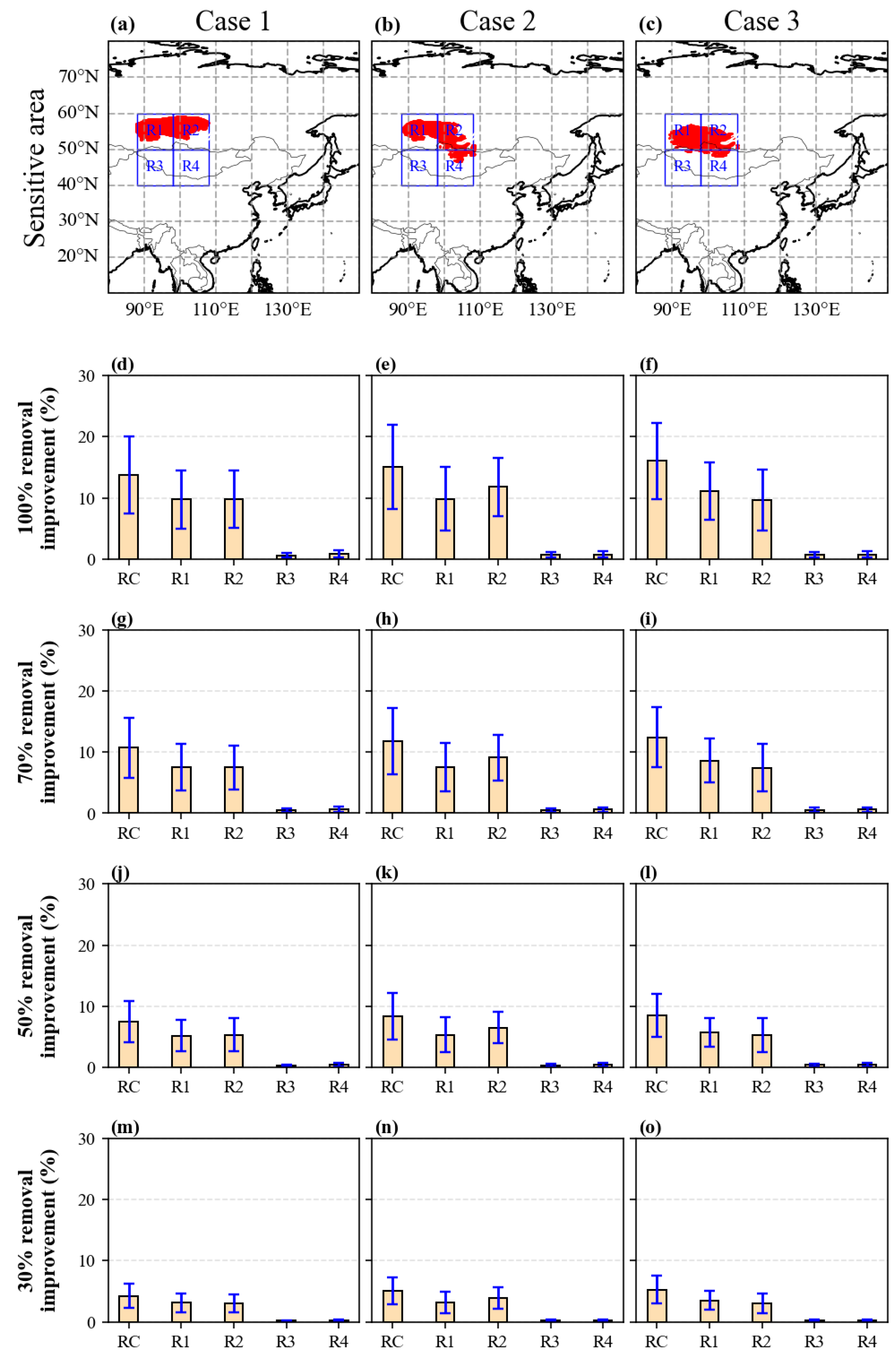
Figure 5g–i indicate that the patterns of the optimal initial errors exhibit pronounced spatial localization, which motivates the identification of targeted observation sensitive areas. More specifically, based on the dry-energy norm, the 1600 grid points with the largest error amplitudes are selected for each case (accounting for approximately 2% of the total domain grid points) to constitute the sensitive region of CNOP-type optimal initial errors (RC). As shown in Figure 12a–c, the RC spatial distribution exhibits remarkable consistency, with all three cases steadily located along the upstream pathway of the cold-vortex formation and development region. This spatial distribution is dynamically reasonable. Previous studies have shown that NECV activity is closely linked to upstream precursor disturbances and Rossby wave-energy propagation along the Eurasian mid-latitude waveguide. In addition, jet-entrance regions often favor perturbation growth through enhanced baroclinic conversion and upper-level flow interaction [36]. To verify the effectiveness of RC in improving forecast skill, four additional comparison subdomains (R1–R4), independent of the error-growth analysis, are manually selected (indicated by blue boxes). Based on these regions, a series of OSSEs is designed to quantitatively evaluate the forecasting improvement of reducing initial errors in different regions.

First, the initial field ${\mathrm{X}}_{\mathrm{in}}$ is used as model input to obtain the reference forecast field ${\mathrm{F}}_1 ={ \mathrm{M}}_{\mathrm{t}}\left({\mathrm{X}}_{\mathrm{in}}\right)$. Then, a random perturbation field is sampled from a standard normal distribution and constrained to 0.3 times the standard deviation, denoted as ${\mathrm{x}}_{\mathrm{re}}$. This perturbation is added to the initial field, and Pangu-Weather is used to generate the resulting forecast ${\mathrm{F}}_2 ={ \mathrm{M}}_{\mathrm{t}}({\mathrm{X}}_{\mathrm{in}} + {\mathrm{x}}_{\mathrm{re}})$. Furthermore, by selectively removing errors in the sensitive regions (RC and R1–R4) and re-running Pangu-Weather, the resulting forecast is obtained as ${\mathrm{F}}_3 = {\mathrm{M}}_{\mathrm{t}}({\mathrm{X}}_{\mathrm{in}} +{ \mathrm{x}}_{\mathrm{ren}})$. It should be noted that the forecast error in this study is computed using the geopotential height field at 500 hPa. To quantify the degree to which reducing initial perturbations in a specific region suppresses error growth, the regional improvement rate is computed as:

$${\mathrm{I}}_{\mathrm{r}} = {\displaystyle \frac{\left|{\mathrm{F}}_2 - {\mathrm{F}}_1\right| - \left|{\mathrm{F}}_3 -{ \mathrm{F}}_1\right|}{\left|{\mathrm{F}}_2 - {\mathrm{F}}_1\right|}} \times 100\% ,$$

(7)

The value of $I_r$ provides a direct comparison of the relative effectiveness of enhanced observations across different regions under identical initial-error conditions. To avoid randomness associated with individual perturbations, 50 independent perturbation experiments are conducted for each NECV case. During the OSSEs, errors are removed in RC and in the four comparison regions R1–R4 for each perturbation field, resulting in a total of $5 \times 50 = 250$re-forecast experiments. The final standard deviation maps are based on statistics from all experiments.

The statistical results shown in Figure 12d–f further confirm that, in all three cases, targeted observations within RC—by effectively reducing initial errors—produce the most substantial forecast improvements. Compared with R1–R4, correcting the initial errors within RC produces much larger forecast improvements. Under the idealized assumption that all initial errors in the sensitive region are removed, the mean improvement reaches about 13%. In contrast, the improvements associated with R3 and R4 are very small in all experiments.

The experiments with partial error removal show similar results. When 70%, 50%, or 30% of the initial errors within RC are removed, the forecast improvements remain consistently larger in the RC region than those obtained for R1–R4. As the proportion of removed errors decreases, the improvement gradually weakens. However, RC still maintains a clear advantage over the artificially selected regions.

4. Discussion

The present study suggests the feasibility of combining a deep-learning forecasting model with a CNOP-based framework to diagnose NECV predictability and targeted observation sensitivity. For the selected NECV cases, Pangu-Weather exhibits forecast skill that is generally slightly superior to ECMWF-IFS, which supports its use in subsequent nonlinear sensitivity experiments. The identified optimal initial errors are mainly concentrated upstream of the cold vortex and near the entrance region of the upper-level jet. Subsequently, these regions are recognized as targeted observation sensitive areas for NECV prediction. Perturbation kinetic-energy budget analysis indicates that baroclinic energy conversion is the dominant mechanism for forecast-error growth. OSSEs further suggest that constraining initial errors within these sensitive areas can improve cold-vortex forecast skill by up to approximately 13% under idealized conditions, indicating their potential practical value for targeted observing strategies over Northeast Asia.

This study helps address a gap in previous research by providing, to our knowledge, the first CNOP-based predictability analysis of NECVs. More broadly, the results suggest that predictability diagnostics can also be applied to artificial intelligence (AI) forecasting systems. Compared with conventional NWP-based studies, the use of Pangu-Weather offers much higher computational efficiency, making large-sample perturbation experiments and sensitivity analyses more practical. The overall consistency between the identified sensitive regions and previous dynamical studies further suggests that AI-based frameworks can capture physically meaningful sources of forecast uncertainty and may provide an efficient new tool for future predictability research.

Several limitations should also be noted. First, Pangu-Weather remains a black-box model, and its internal forecast processes cannot yet be fully interpreted in dynamical terms. Second, the CNOP-type perturbations are identified through sampling-based search rather than formal optimization, and therefore represent practical approximations to the theoretical optimum. Third, because the OSSE framework is idealized, the reported forecast improvement should be regarded as a theoretical upper bound. In practice, factors such as instrument errors and uneven observational coverage may reduce the actual achievable improvement. In addition, the evaluation dataset is limited in both temporal coverage and sample size, as only May–August 2022 data and three representative NECV cases are examined. Model performance may also vary across seasons, regions, variables, and synoptic conditions. Finally, only one deep learning model is investigated here. Future work should include larger samples, longer evaluation periods, partial-error reduction scenarios, and cross-model comparisons among multiple AI and NWP systems.