


Abstract
A study of agricultural yield sensitivity in Peru to climate variations is conducted from 1961 to 2024 to identify climate drivers and statistical tools for early warning and risk management. The statistical basis is year-on-year change in standardized crop yield rate (CYR) across the southeastern highlands of Peru 7–15° S, 70–77° W. Crops favoring La Nina include citrus, cotton, fruit, and sugar-cane. Based on temporal and spatial correlation and composite analysis, our findings indicate that (i) east Pacific and Caribbean sea temperatures and Atlantic upper winds provide advance warning signals of CYR fluctuations; (ii) during El Niño, the subtropical jet subsides over the Peruvian highlands, raising temperatures and lowering humidity; (iii) during La Niña, cooler temperatures conspire with rising motion and beneficial rains; and (iv) CYR fluctuations account for 26% of macro-economic variance, ~$66 B at the current value. Bringing technological information to agricultural decision making will improve resilience and help meet the twin challenges of a growing population and changeable climate. Adaptive measures are suggested to take advantage of Southern Oscillation’s influence on austral summer weather and subsequent annual crop yield.
1. Introduction
Climatic conditions naturally exert control over environmental resources, shaping both ecosystems and livelihoods. Efforts to optimize agrarian production while minimizing climate risks are an ever-present challenge for Peru [1,2,3,4]. Scientific knowledge, when well applied, can support management solutions that balance productivity, sustainability, and resilience. Several theories integrate biophysical shocks, adaptive behavior, and strategic planning to build effective policy and resilience in agricultural systems under climate variability [5,6,7,8,9,10,11]. In this context, understanding past and current climate patterns is essential to anticipating seasonal anomalies, reducing vulnerability, and guiding adaptive management. While long-range forecasts offer opportunities to anticipate climate behavior, unexpected droughts or floods continue to adversely affect rural prosperity and food security [12]. Changes in the frequency and intensity of El Niño–Southern Oscillation (ENSO) are a constant global threat compounded by climatic trends, although concentrated in the equatorial Pacific [13], hence the importance of accurate model outputs and implementation of mitigation measures to minimize adverse effects and improve environmental sustainability, public health, and food security [14,15].
Peru, with its diverse geography ranging from arid coastal plains to high Andean plateaus and Amazonian lowlands, is very exposed to climatic variability. Agriculture remains central to its productivity, with half of agricultural effort in the east-facing highlands > 1500 m [16], one-quarter in the tropical Amazon basin (<10° S), and one-quarter in the subtropical western margin [17]. The agricultural sector contributes around 7% to gross domestic product but employs 30% of the labor force [18,19]. However, agricultural land is limited: half of Peru is forested; 15% is used for livestock grazing; and only about 7% is dedicated to crop farming, mostly coffee, maize, tubers, vegetables, and fruits [20]. Irrigated farming is confined to coastal valleys, while rain-fed systems dominate the interior. Therefore, Peru’s diverse climates, altitude-driven agricultural systems, rich agrobiodiversity, and exposure to climatic fluctuations motivate our research to underpin sustainable agrarian adaptations [21].
Despite significant progress in food production and export, Peruvian agriculture faces persistent challenges. Infrastructure gaps, limited financial access, and under-utilized technology tend to hinder efficiency, particularly among two-thirds of farmers who operate small, non-mechanized plots in the highlands [20,22]. The distance between centers of production and consumption is a key issue: half of the country’s 34 million people live in coastal cities [23] and rely on food brought from the verdant highlands to the western desert. There is rapid rural-to-urban migration that fosters dependency on external supply chains [24]. Since 2003, governmental efforts have addressed agricultural sensitivity to climate [25]. Historical studies [26] and recent analyses [16,27,28] underscore how the El Niño–Southern Oscillation (ENSO) causes opposing weather over eastern and western Peru, compromising food security [29]. El Niño events often result in coastal flooding and highland drought, while La Niña brings rainy conditions to the Altiplano. These patterns affect farming decisions, crop yields, and water supplies [30,31]. Most studies have found a lagged response of annual crop yields to prior summer climate, yielding early warning systems based on oceanic precursors. However, gaps remain in understanding atmospheric responses and impacts.
This study addresses uncertainties through a statistical evaluation of crop yield sensitivity to summer climate conditions across Peru. It aims to identify both simultaneous and leading indicators of variability to inform pre-season decision-making. Peru has an established tradition of agro-climate monitoring, including long-term datasets from Peru’s weather service, which helps with validation of climate–yield relationships [32,33].
In Section 2, the data analysis methodology, climate indices, and crop production are described. Section 3 presents (i) the temporal analysis of crop yields, (ii) field correlations and composites to identify climate drivers, and (iii) statistical outcomes relevant to early warning and risk management. Section 4 concludes with implications for climate-sensitive agriculture in Peru and how technological innovation can reduce rural vulnerability. This work is part of a multi-faceted study of Peru’s climate sensitive resources: (i) macro-economic performance, (ii) agricultural yield, (iii) fisheries production, and (iv) gradients in coastal weather, identified at a workshop held at the National University of Trujillo in July 2025.
2. Data and Methods
This study of Peruvian agricultural links with regional climate variability uses a multi-variate approach that quantifies the precursors and drivers of crop yield fluctuations. Peru is on the doorstep of ENSO and its amplified response has global implications.
2.1. Agricultural Data
Annual crop yield data for Peru were obtained from the UN Food and Agricultural Organization [20], covering the period 1961–2024. This dataset includes national-level statistics for major crop groups (cereals, vegetables, fruits, tubers, legumes, oilseeds, and industrial crops). To normalize disparate crop types, the yield contributions were analyzed separately and then standardized (subtracting the overall mean and dividing by the standard deviation) and aggregated to form a combined yield (all-crop average), providing a unified measure of national agricultural performance.
The year-on-year change in the combined yield was calculated to derive the crop yield rate (CYR). This metric reflects interannual variability and is more sensitive to climate-induced productivity than absolute yields, which have trends due to technology. The CYR was subjected to statistical analysis to characterize its probability distribution and extremes, and regional sensitivity to the austral summer climate.
2.2. Correlation Analysis
The individual crops and aggregated CYR time series 1962–2023 were correlated with the Southern Oscillation Index (SOI) and Niño3 Sea Surface Temperature (SST), representing equatorial Pacific variability. Time–space or point-to-field regressions were calculated between the CYR and January–March fields of CRUv4 gridded rainfall [34], global sea surface temperature (SST), and sea level pressure (SLP) from the Hadley Centre [35]. Our focus is austral summer, when crops are most sensitive to local climate and highland temperatures stay above 10 °C [16].
Statistical significance was evaluated using correlation thresholds based on the effective degrees of freedom from the sample size and autocorrelation (persistence). For datasets covering 60+ years, a Pearson correlation coefficient of R > |0.20| yields ~ 90% confidence. For shorter records (1980–2023), a coefficient threshold of R > |0.25| is required.
Satellite-derived variables employed in the analysis included (i) Outgoing Longwave Radiation (OLR), used as a proxy for convection and cloud cover [36], and (ii) vegetation color fraction or chlorophyll fluorescence, NDVI [37], representing landscape condition. These fields were analyzed during the Jan–Mar window using point-to-field correlation with the national CYR to identify regions having greater climate–yield linkages.
2.3. Mapping of Composite Anomalies
To explore the climate mechanisms underlying fluctuations in agricultural productivity, the CYR time series was ranked and categorized into ten down-turns (1963, 1964, 1971, 1972, 1979, 1983, 1990, 1992, 1998, and 2015) and ten up-turns (1970, 1984, 1993, 1994, 1999, 2001, 2005, 2014, 2018, and 2022), based on standardized departures exceeding ±0.3 σ.
Atmospheric and oceanic fields were averaged for these down-turn and up-turn seasons to identify the prevailing circulation and thermodynamic anomalies using NCEP-1 reanalysis for winds, vertical motion, specific humidity, and surface air temperature [38]; and GODAS ocean reanalysis for subsurface ocean currents and thermal structure [39].
Composite anomaly maps and vertical cross-sections (averaged E–W over Peru 7–15° S) were constructed to examine both zonal and meridional circulation anomalies, for standing waves in the upper ocean and atmosphere, overturning Walker circulations, and the impact of subtropical anticyclones. Events were grouped by ENSO phase (El Niño and La Niña) to isolate non-linear atmospheric responses, consistent with prior studies on tropical–extratropical coupling [40,41,42].
2.4. Forecast Potential and Early Warning Signals
To assess the predictability of crop yield fluctuations, correlations were performed using climatic variables in the preceding October–December (OND) season. Gridded global correlation maps were generated for SST, SLP, OLR, and rainfall to detect teleconnections with subsequent year-on-year changes in Peru crop yield. For early-warning application to distinguish mild vs. severe down-turns, the sample size is limited and correlations should exceed |0.50| to achieve 90% confidence.
Additional analyses considered (i) individual crop yields vs. Niño3 SST, to assess contrasting sensitivity; (ii) numerical forecast skill, comparing CRUv4 observed Jan–Mar rainfall over Peru (7–15° S) with model predictions from ECMWF v5 in the preceding Oct–Dec; and (iii) comparison of CYR and Peru macro-economic growth rate, using data from the World Bank, to evaluate agricultural contribution to the national economy. From these outcomes, recommendations are formulated to assist farm managers and government services to improve adaptation and stabilize market forces.
2.5. Assumptions and Limitations
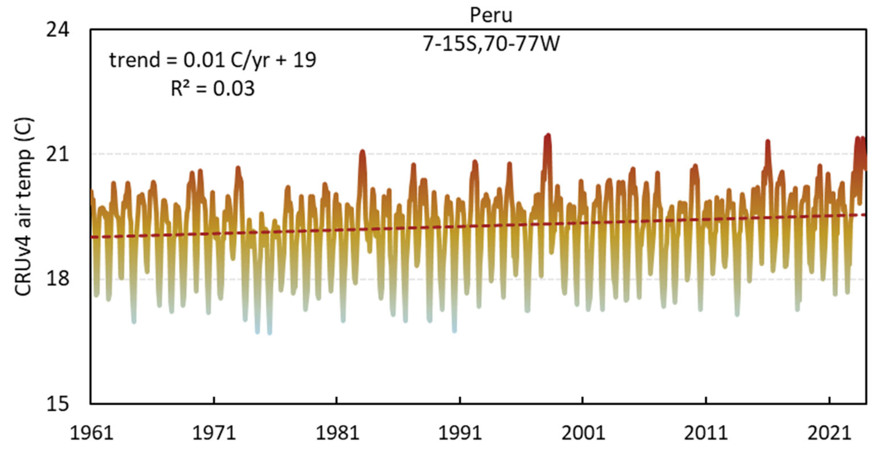
The following assumptions underpin the methodology: (i) FAO-reported national yield statistics are representative of true agricultural performance; (ii) a unified CYR metric reasonably captures the climate sensitivity of diverse crops across heterogeneous landscapes; (iii) global reanalysis data accurately portray climatic conditions over Peru’s varied and complex terrain; (iv) austral summer (Jan–Mar) weather anomalies modulate annual yields, due to phenological sensitivity and plant–harvest cycles; (v) our methods are applicable elsewhere, given reliable CYR data; and (vi) global warming effects are a small (R2 = 0.03) compared with seasonal variability (cf. Appendix A). Thus, trends have been retained in temporal analyses, acknowledging the combined influence of climate change and interannual variability. While this enhances realism, it may conflate multi-decadal impacts.
3. Results
3.1. Peru Agricultural Yield and Temporal Characteristics
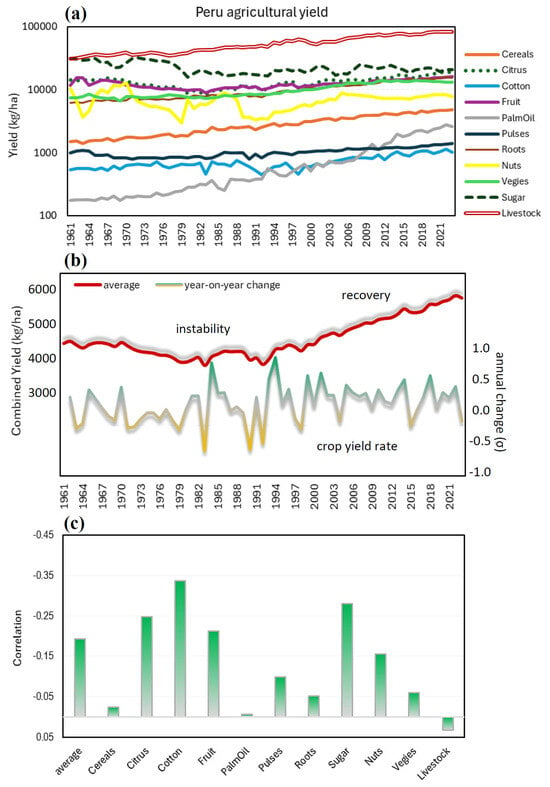
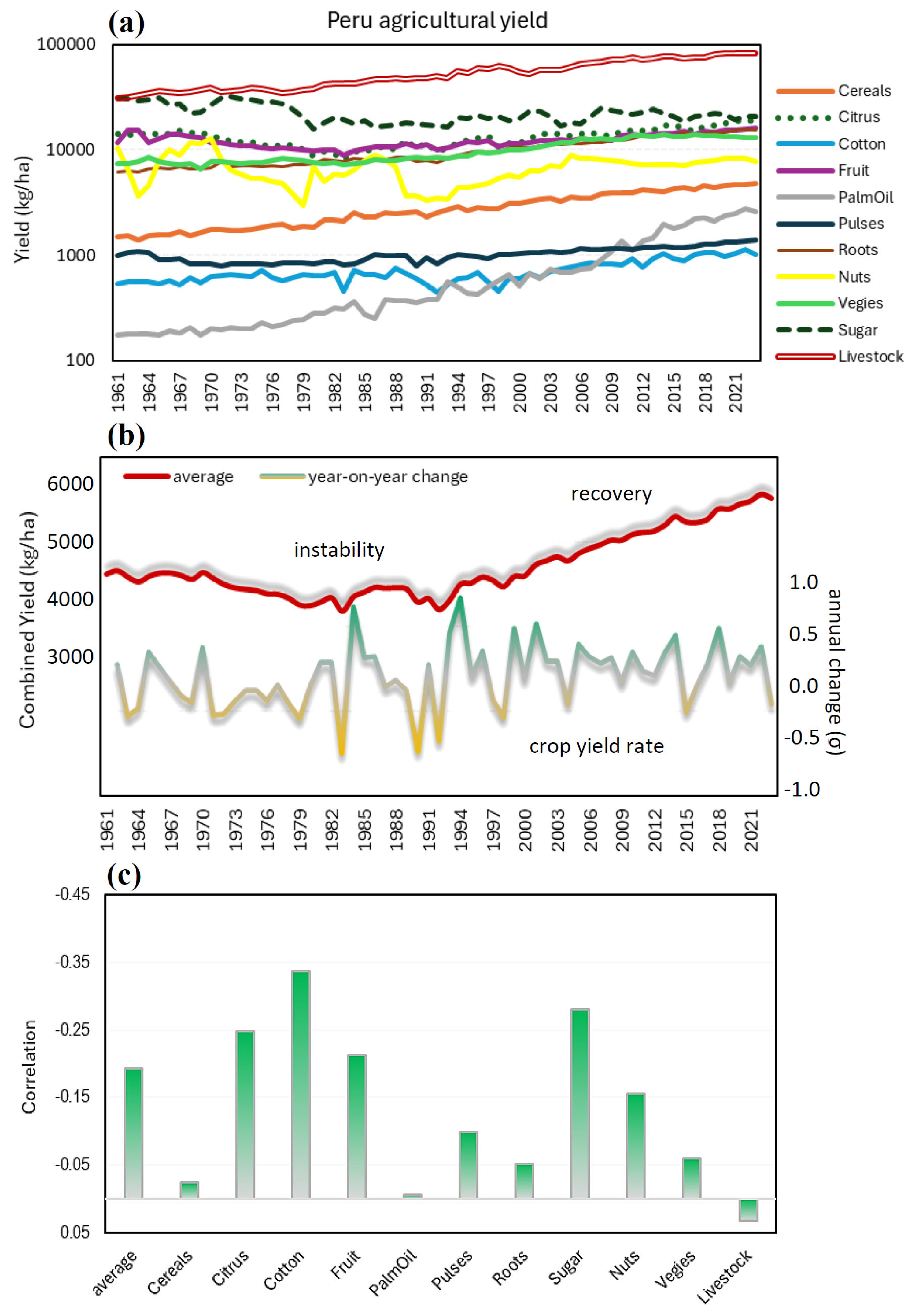
Peru’s annual agricultural output from 1961 to 2024 (Figure 1a) reveals three distinct phases: (i) relatively stagnant production during the 1960s to early 1980s, (ii) a modest upward trend through the 1990s and early 2000s, and (iii) more pronounced interannual variability in the last two decades. These changes align with periods of political stabilization, market liberalization [43,44,45,46], and gradual adoption of improved crop varieties and technologies throughout Peru [47].
Figure 1.
(a) Time series of FAO agricultural yields in Peru, note that sugar-cane is divided by 10, (b) combined (averaged standardized) values (red) and year-on-year change ‘crop yield rate’ (sigma), (c) Pearson correlation coefficients for individual crop yield fluctuations versus the preceding summer (Jan–Mar) 1961–2023 Pacific Niño3 sea temperature, where R < −0.20 is significant at 90% confidence (inverted scale).
After standardizing and averaging across all major crop groups, the combined yield (Figure 1b) shows a gradual increase in production since the mid-1980s. However, the interannual variability remains pronounced, with several sharp declines—often associated with drought or flood years—and rebounds in subsequent years. Oscillations in year-on-year change (CYR) have no trend and suggest long-term resilience but short-term vulnerability to climatic shocks.
Figure 1c illustrates the Pearson correlation coefficients between the preceding summer (Jan–Mar) Niño3 sea surface temperatures (SST) and annual yield fluctuations for key crops. Most crops exhibit negative correlations, indicating that La Niña-like (cool) conditions in the tropical east Pacific tend to favor higher yields. Notably: strong negative correlations (R < −0.4) are observed for sugar-cane, citrus, fruit trees, and cotton, suggesting that these crops are particularly sensitive to moisture availability and temperature anomalies during the austral summer growing season.
Moderate to weak responses are seen for cereals and palm oil, possibly reflecting mixed growing zones and better drought tolerance. Livestock productivity, in contrast, shows a positive correlation with Niño3 SST, indicating enhanced pasture conditions or disease reduction during ENSO warm phase, possibly due to milder winters or improved fodder access in El Niño years.
This crop-specific analysis underscores a broad sensitivity of the agricultural sector to east Pacific climate variability and the need for adaptation strategies.
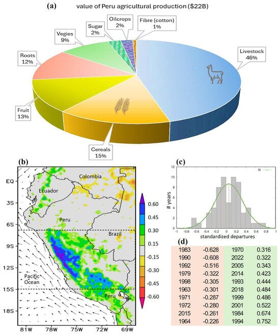
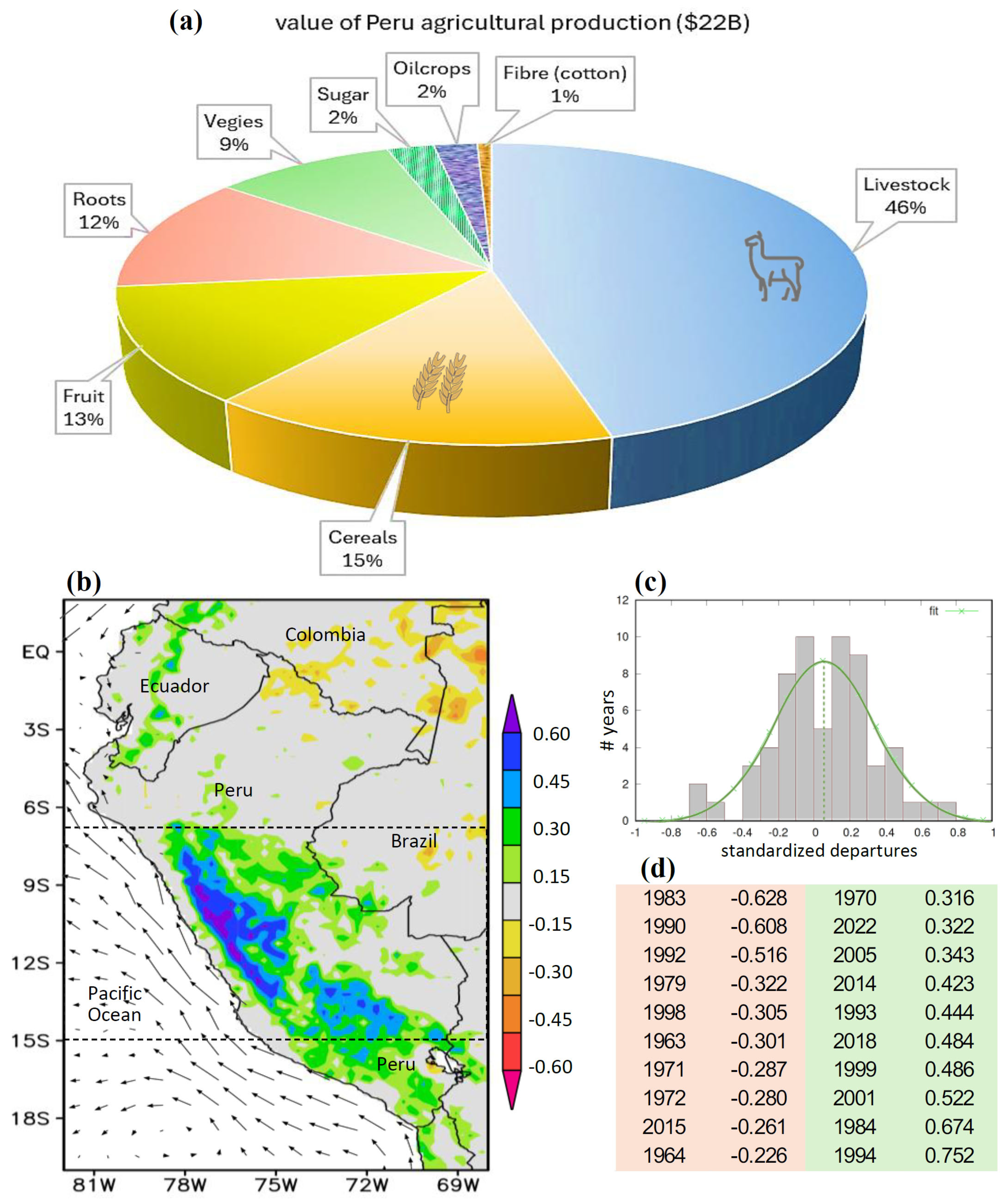
A breakdown of Peru’s $22 billion agricultural economy illustrated as a pie chart (Figure 2a) shows that livestock products (meat, dairy, and wool) dominate with a 46% share, followed by cereals (15%), fruit (13%), roots and tubers (12%), and vegetables (9%). This economic structure emphasizes the importance of pasture quality, particularly in the highland regions, with dual reliance on both rain-fed crops and livestock production.
Figure 2.
(a) Pie chart of sectoral % contributions to Peru agricultural value, FAO data averaged for 2018–2023. (b) CYR correlation with Jan–Mar 1980–2023 satellite vegetation color fraction (shaded) and GODAS 1–100 m ocean currents (vectors, largest 0.6 m/s), representing an up-turn in production. (c) Histogram of crop yield rate vs. normal distribution. (d) Ranked down-turn (brown) and up-turn years of crop yield rate (σ). Dashed area in (b) refers to cross-sections in Figure 5.
The CYR’s correlation with Jan–Mar satellite-derived vegetation color fraction (Figure 2b) reveals a statistically significant spatial pattern. Positive correlations (R > 0.30) are strongest over the east-facing highlands and the southern Altiplano (south of 7° S)—areas characterized by seasonal rainfall, elevation gradients, and limited irrigation infrastructure. These regions are particularly sensitive to climatic anomalies during summer months, with vegetation health serving as a proxy for crop and pasture condition.
In contrast, the Amazonian lowlands in northeastern Peru exhibit weak or no correlation with CYR. This insensitivity reflects both the dominance of forestry over agriculture in this zone and the more stable rainfall regime driven by the Intertropical Convergence Zone (ITCZ) rather than ENSO variability.
Marine analyses reveal interesting patterns: the northward flow of cold coastal currents accentuated by La Niña is associated with agricultural up-turns, while reversals in current direction during El Niño years are linked to down-turns, due to soil water deficits across the eastern highlands. These ocean–atmosphere interactions appear to play a modulating role in agricultural productivity.
The frequency distribution of the CYR (Figure 2c) is broadly symmetric, indicating that up-turns and down-turns have similar frequencies of occurrence. The histogram exhibits clustering near ±0.2 σ, representing modest fluctuations. Deviations greater than ± 0.4 σ are infrequent but impactful. Thus, agricultural production in Peru rebounds from down-turns due to ENSO transitions and external factors such as government recovery programs and market corrections to offset supply–demand imbalance.
A list of the top-10 down-turn and up-turn CYR years (Figure 2d) identifies those for further investigation in composite analyses. Down-turns in 1963, 1964, 1971, 1972, 1979, 1983, 1990, 1992, 1998, and 2015 tend to align with El Niño events and associated inland drought and coastal flood. Up-turns in 1970, 1984, 1993, 1994, 1999, 2001, 2005, 2014, 2018, and 2022 tend to align with La Niña episodes and improved climatic conditions. These years form the basis for subsequent analysis and predictor evaluation.
3.2. Correlation and Composite Patterns
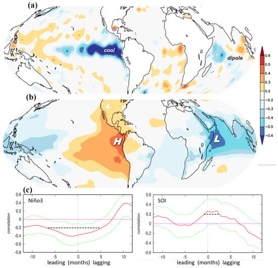
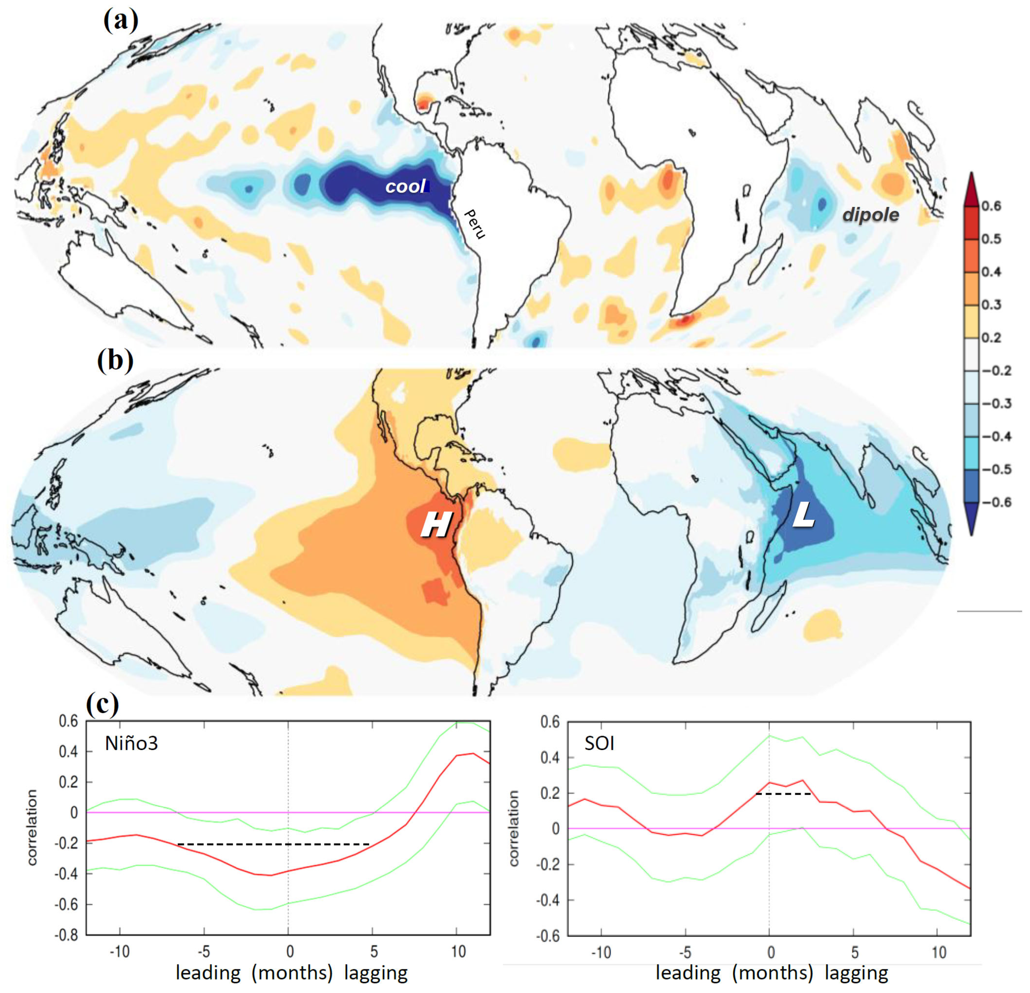
To identify the large-scale climate patterns influencing Peruvian agriculture, we applied point-to-field correlation mapping between the crop yield rate (CYR) and global atmospheric–oceanic datasets during the key growing season (January–March). The outcome in Figure 3a,b reveals spatial signals of climatic influence.
Figure 3.
Crop yield rate correlated with Jan–Mar fields of (a) near-surface sea temperature and (b) sea level air pressure, 1961–2023, R > |0.20| significant at 90% confidence; patterns represent an up-turn in agricultural production. (c) Lag-correlation of Niño3 sea temperature (left) and Southern Oscillation air pressure time series with CYR, zero is Jan–Mar, the environment leads, dashed is significant, and green lines are upper and lower quintiles.
A most significant correlation emerges in the tropical eastern Pacific off Ecuador and the Galápagos Islands. In this region, cooler sea surface temperatures (SSTs) are associated with higher CYR values, indicating that La Niña enhances Peru crop yields, while El Niño has a negative effect on agricultural productivity. This relationship is robust, with correlation coefficients > 0.4 in the Niño3 region and surrounding coastal zones, consistent with previous studies on ENSO impacts in western South America [41].
A secondary SST pattern is observed over the distant tropical Indian Ocean, showing a cool-west/warm-east pattern known as the Indian Ocean Dipole (IOD). In austral spring and summer when the west/east Indian Ocean is cooler/warmer than average, the CYR tends to be higher. Naturally, the remote Indian Ocean influence is weaker than the Pacific, yet the pattern indicates a teleconnection involving regional moisture transport by the Walker circulation over South America.
In the atmospheric domain (Figure 3b), sea level pressure (SLP) fields indicate that favorable crop yield conditions are associated with higher-than-average pressure over the tropical east Pacific and lower-than-average pressure over the west Indian Ocean. This pressure dipole reflects a positive phase Southern Oscillation, which reinforces southeasterly winds and upwelling along the coast of Peru, typical of La Niña episodes.
Temporal lag-correlation analysis between the CYR and Pacific SST/atmospheric indices (Figure 3c) shows that cool SSTs in the Niño3 region and positive Southern Oscillation Index (SOI) values correlate significantly with up-turns in crop yield six months in advance. Thus SST anomalies observed during the October–December (OND) season can serve as reliable early warning indicators for the following year’s agricultural performance, as noted in [28].
This lagged relationship supports the development of seasonal forecasting tools for Peruvian agriculture, offering a valuable opportunity for government agencies, farmers, and suppliers to anticipate potential down-turns (El Niño years) or up-turns (La Niña years) and take pre-emptive action to manage risk.
To further understand how local weather patterns translate global climate signals into yield variability, we analyzed regional point-to-field correlations and composite anomalies during the growing season.
Figure 4a,b show that during up-turns in CYR, there is a consistent pattern of enhanced cloudiness and increased rainfall over southeastern Peru, especially along the east-facing highlands and the Altiplano. This region is crucial for smallholder agriculture, and its sensitivity to seasonal precipitation explains much of the interannual variability in national crop yield.
The atmospheric circulation favoring crop yield comprises weak convergent low-level westerlies (Figure 4c) and strong upper-level easterlies (Figure 4d), supporting upward motion and cloud development over the highlands. This climate pattern enhances soil moisture; moderates surface temperatures; and extends the growing season for key crops such as maize, potatoes, and quinoa.
In contrast, down-turns are associated with a strengthened subtropical jet-stream, evident in composite height-sections of wind and humidity fields averaged 7–15° S (Figure 5a,b). Subsidence prevails over the Andes, leading to dry, warm downslope winds that deplete soil moisture and inhibit crop growth across the Altiplano. Coastal zones are characterized by reduced upwelling, warmer SSTs, and high humidity, typical of El Niño events that bring damaging floods in Jan–Mar season.
Figure 4.
CYR correlation with Jan–Mar fields: (a) CRU4 gauge rainfall (1961–2023), (b) satellite net OLR (1980–2023), and (c,d) NCEP-1 lower- and upper-level wind (1961–2023), representing an up-turn in production, vector key (m/s). Scale adjusted in (a,b) so blue is moist, and dashed in (a) is the target area of model forecasts in Figure 6e.
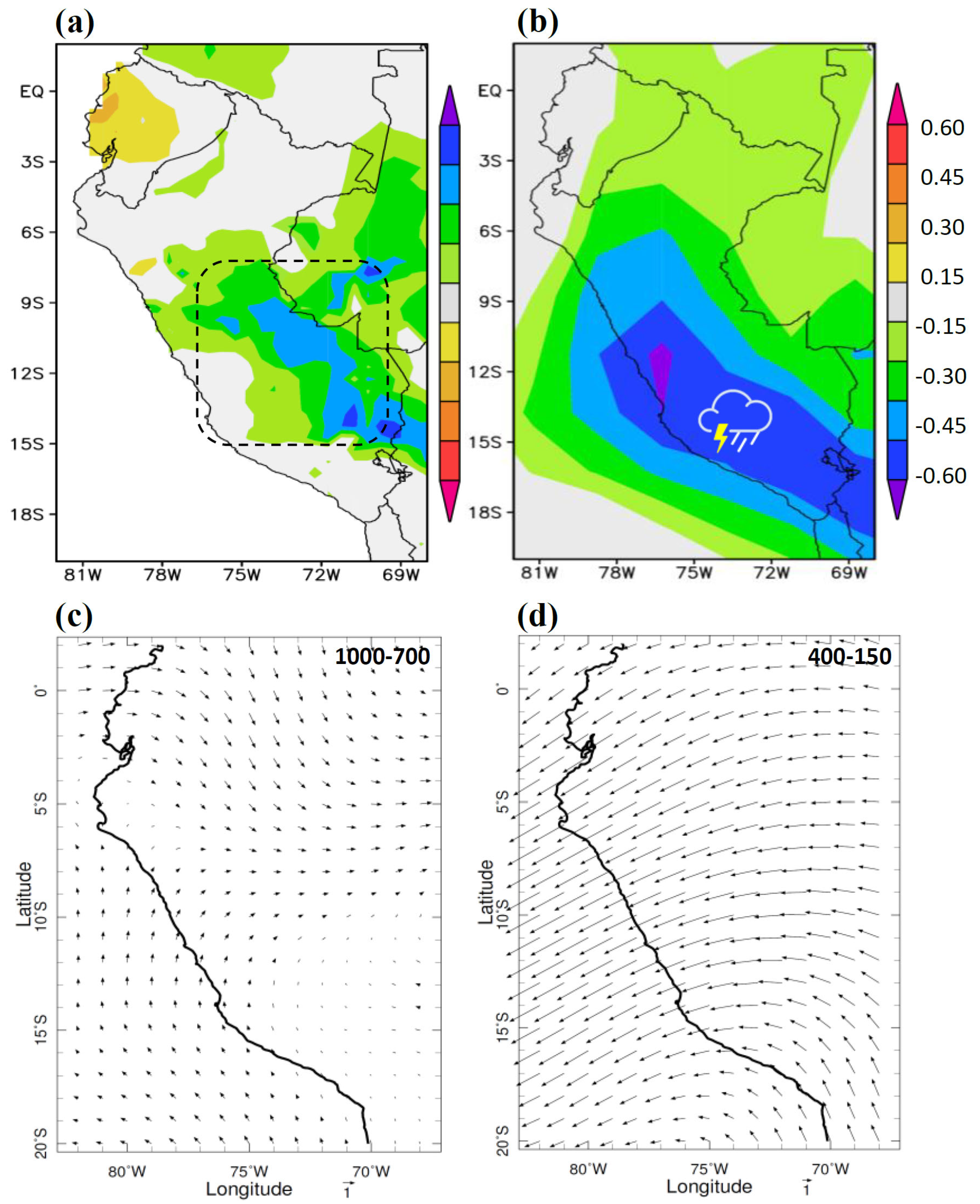
Figure 5.
Composite height-section (averaged 7–15° S) of Jan–Mar zonal circulation (vectors) and specific humidity anomalies (green contours) and surface temperature anomalies (bars, lower) for (a) 10 down-turn years and (b) 10 up-turn years, based on the listing in Figure 2d. Key features are labeled, vertical motion is exaggerated, and largest vector is 2 m/s. Vertical axis is pressure, corresponding to heights from 0 to 12 km with a proportionate topographic profile. Anomalies refer to group average minus Jan–Mar 1970–2024 mean.
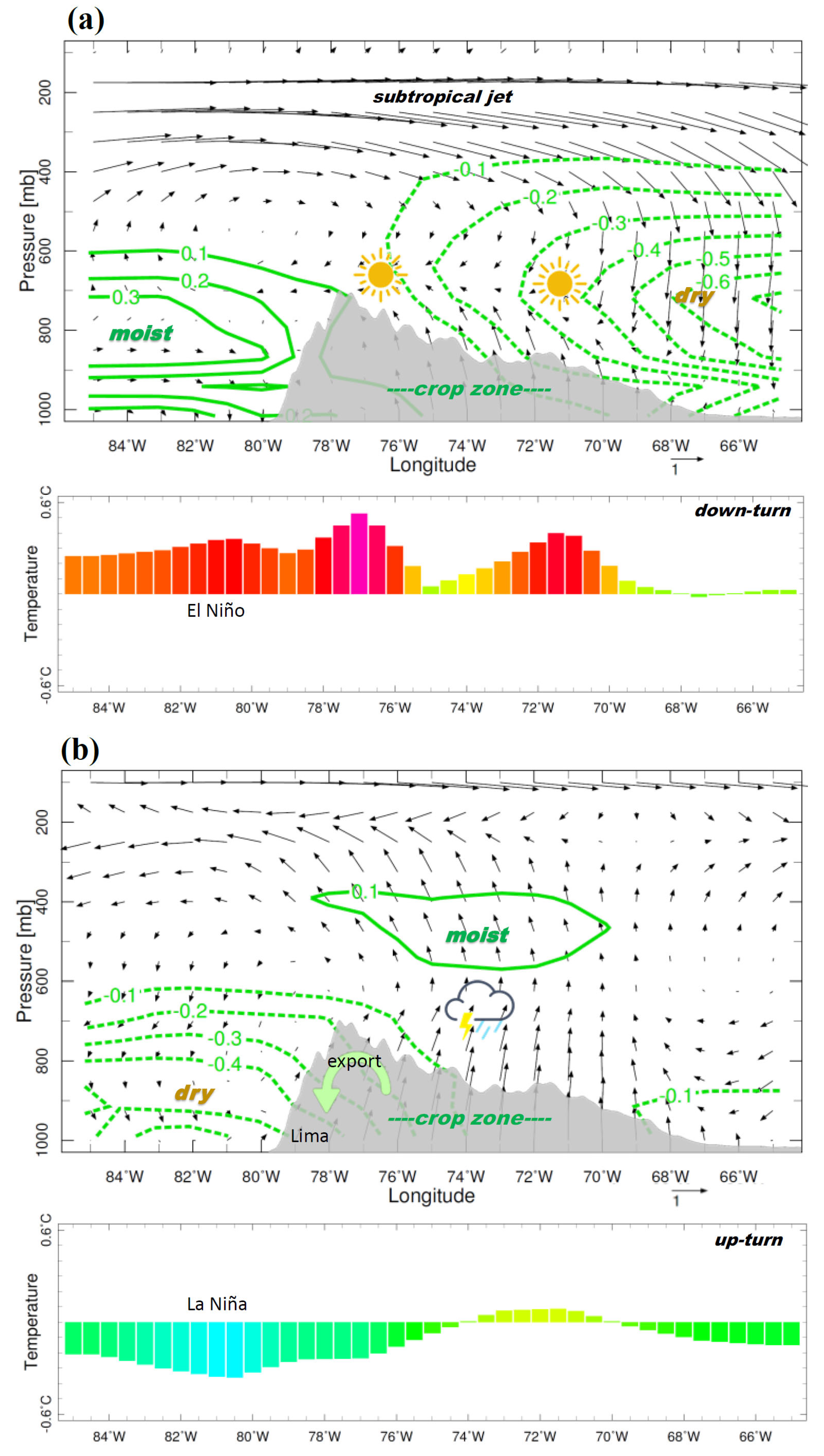
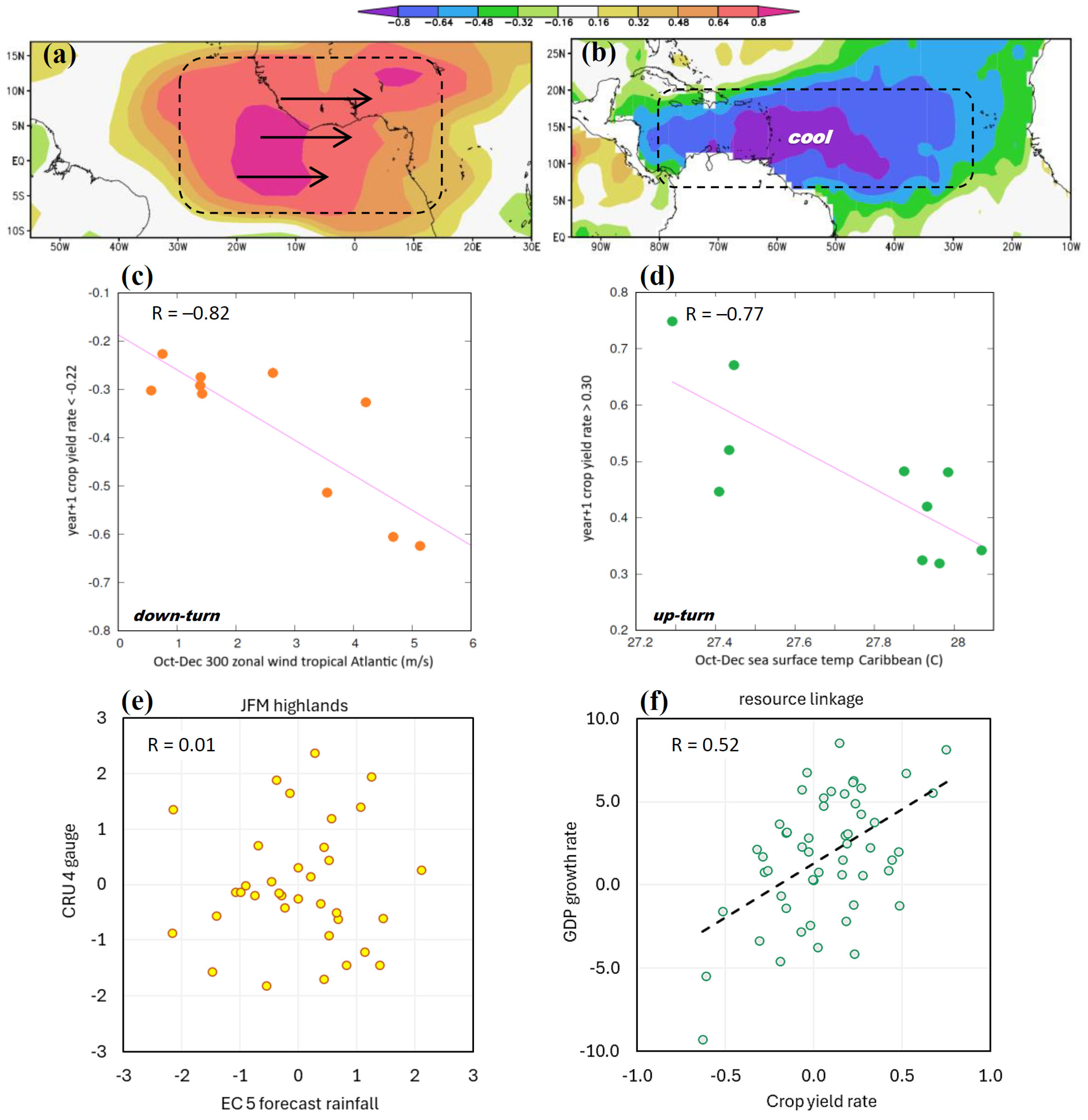
Figure 6.
Correlation maps in the preceding Oct–Dec 1961–2023 to identify predictors (dashed) for advance warning: (a) tropical Atlantic 300 hPa zonal wind for down-turns <−0.22 and (b) Caribbean sea surface temperature for up-turns >0.30. Scatterplots of year+1 crop yield rate versus (c) tropical Atlantic wind and (d) Caribbean SST in the preceding austral spring, N = 10. Scatterplots of (e) EC 5 coupled numerical model December forecast of Jan–Mar highlands rainfall vs. gauge, 1980–2023 (no skill); (f) Peru CYR vs. macro-economic growth rate with linear regression fit, 1970–2023.
Naturally, up-turns exhibit the opposing pattern: coastal SSTs are cooler, marine winds are equatorward, and rising motion dominates the interior and Altiplano. These conditions limit the risk of crop disease, while supporting moisture retention and stable temperatures during critical stages of phenological development.
Our correlation and composite outcomes indicate that La Niña conditions (cool Niño3 and positive SOI) are favorable for Peru crop yields, especially in the eastern highlands Altiplano. As expected, ENSO teleconnections are the dominant global driver of Peruvian agricultural variability, with global surface temperature and pressure anomalies detected six months in advance. High-yield years are linked to increased rainfall and upward motion over the Altiplano, while low-yield years are characterized by dry, subsiding flow over the interior highlands. Secondary patterns in the Indian Ocean serve to indicate the atmospheric bridge associated with a global wave-2 zonal circulation [48] that is favorable to Peru. The most important of which is the upper-level subtropical jet, a thermal wind response to meridional temperature gradients established by ENSO. These results lead us to early warning signals and targeted climate adaptation strategies.
3.3. Prediction and Adaptation
To better anticipate fluctuations in Peru’s agricultural output, we consider the preceding Oct–Dec environmental patterns ’trained’ on the two composite groups. Following comprehensive exploratory research, key advance warning signals are uncovered. Down-turns are preceded by acceleration of upper-level westerlies over the tropical east Atlantic (10 S–15 N, 30 W–15 E, Figure 6a,b) with a linear regression fit of R −0.82. Up-turns are preceded by cooling of the Caribbean Sea (7 N–20 N, 80 W–30 W, Figure 6c,d) with a fit of R −0.77. Surprisingly, the Southern Oscillation influence on Peru’s agriculture is pre-conditioned by signals originating from the Atlantic.
Statistical forecasts based on prior ocean–atmosphere variables [49] could be complemented by numerical forecasts [50]. However, validations of ECMWFv5 model outputs against CRUv4 rainfall (Figure 6e) indicate poor skill for austral summer rains over Peru (7–15° S) and beyond [51,52,53].
What adaptive measures can be implemented? Predictions can be translated into a plan-of-action for agricultural decision makers [25]. However, recommendations would have two implementation streams: 1. for large-scale commercial farmers in the west and 2. for small-scale farmers in the east. It is recognized that the uptake of scientific guidance would trickle-down from the large to small scales. If near-average weather conditions are expected, then normal farming operations would be favored. If an advance warning of a down-turn is publicized, then finance and planted area could be constrained. Large-scale farmers would be encouraged to focus on quality instead of quantity, thus sustaining crop yield and minimizing debt risk and production losses from high temperatures and evaporation [54,55,56,57,58,59]. Short-cycle drought-tolerant crop types would benefit from soil moisture conservation via compost and mulch [60,61]. Farmers can control moisture depletion via irrigation and specialized fertilizers. If an advance warning of an up-turn is publicized, finance and planted area could be expanded to meet increased market demand. Large-scale farmers would be encouraged to focus on quantity and surplus for export [62,63]. Short-cycle crops that are rain-tolerant would benefit from runoff management via terracing during wet spells.
Other short-term alternatives for large-scale farmers include osmo-protectants [64], biostimulants [1], and technology to improve fertilizer application [55]. In the long term, genetic engineering could encourage the use of climate-smart varieties [65].
Small-scale farmers in the east would take note of the uptake of scientific guidance and its value to their large-scale counterparts. They have an arsenal of local solutions to translate scientific guidance into tangible benefits, from a long history of indigenous practices to enhance prosperity [21,66].
Agricultural workers in Peru add value at ~$4000 per capita compared with $8000 in neighboring countries [18]. That under-performance can be boosted with new technology via government services which are already in place [67,68]. Peru’s weather service (SENAMHI) links with state agricultural departments and commercial farm managers via online advisories <www.senamhi.gob.pe/?&p=aviso-meteorologico> → <agrolalibertad.gob.pe/> (accessed on 1 September 2025). Existing advance warning systems could utilize the statistical outcomes presented here, in parallel with long-range numerical forecasts of austral summer rainfall; keeping in mind the wet bias [69] and poor model skill over the Peruvian highlands, as illustrated in Figure 6e.
Market forces will drive commodities in down-turns and equities in up-turns, helping to stabilize macro-economic volatility [70]. As this happens, efforts can be directed at improving infrastructure to ensure that excessive dry and wet spells can be overcome. Boosting the early warning system will help put mitigation measures into action [2] and contribute to agricultural extension services [4]. Peru’s varied landscape affords opportunities to mitigate global warming (cf. Appendix A) by strategically shifting farming effort to the optimal phenological range.
4. Concluding Discussion
A study of Peru agricultural yield sensitivity to climatic fluctuations was conducted over the period 1961–2024. Our basis for statistical analyses was the year-on-year change in standardized all-crop yield, formulated by (i) subtracting the overall mean and dividing by the standard deviation for each crop, (ii) averaging all together, and then (iii) subtracting the previous year’s yield from the following year. Although livestock production adds 46% to agricultural value, its contrasting relationship with the Southern Oscillation and known response-delays [71] excluded it from the CYR. The crops most favoring La Niña over El Niño included citrus, cotton, fruit, and sugar-cane. The southeastern highlands of Peru 7–15° S, 70–77° W ‘carried’ the yield signal. We acknowledge methodology limitations that include unstable country-wide reporting and inadequate remote sensing before 1980.
To achieve our scientific goals, agricultural responses to climate were analyzed via correlations and composites. The La Niña ‘pulls’ southeasterly winds from the Amazon, which move upslope and rain. Conversely, the El Niño suppresses the east Pacific cold tongue and ‘pushes’ northwesterly winds onto the coast. As the subtropical jet subsides over the Andes, soil moisture is depleted and crop yields suffer. El Niño floods harm coastal transportation networks and over-saturate crops like sugar-cane.
Our study builds on prior work with an economic focus. Here, crop yields provide the basis for analysis whereas the earlier work [72] utilized changes in Peru’s gross domestic product (GDP). Similar ENSO responses may be noted (La Niña-favorable), which stem from the large contribution that agriculture makes to macro-economic performance. Evaluating the potential for long-range CYR forecasts over the Peruvian highlands, we found strong statistical performance using novel predictors over the Atlantic sector but quite weak numerical performance using operational weather models. In contrast, the statistical prediction of GDP growth rate [72] utilized only Pacific predictors.
New findings which emerged from the CYR analysis include the following: (i) tropical Pacific and Caribbean sea temperatures and Atlantic upper winds provide advance warning signals of agricultural productivity; (ii) the subtropical jet subsides over the Peruvian Altiplano during El Niño, raising temperatures and depressing humidity; (iii) during La Niña, lower evaporation conspires with rising motion and beneficial rains over the highlands; (iv) fluctuations in Peru crop yield cover 26% of the economic variance (Figure 6f), ~$66B at the current value. Thus, indirect effects are extensive and spread from the Altiplano to coastal cities such as Lima.
We understand that commercial farmers will employ technology more readily and that finance and export are important, whereas small-scale farmers are less likely to employ technology until it is proven to work. For small-scale farmers, finance and export are inconsequential, but their production supports municipal markets and well-being throughout Peru.
Adding this scientific information to decision-making would promote resilience to help Peru meet the twin challenges of a growing population and an ever-changing climate. Many universities have experimental farms and liaise with regional agriculture extension programs, so to spread the outcomes generated here. Further work will (i) analyze the major crop regions separately using local datasets, (ii) understand how the Atlantic ‘pre-conditions’ Southern Oscillation influence, and (iii) test the value of our recommended adaptations in local farming operations.
Author Contributions
M.R.J. conceived, analyzed, and wrote the first draft, M.B. re-wrote the paper and added local insights and references. All authors have read and agreed to the published version of the manuscript.
Funding
No direct funding was received for this research.
Data Availability Statement
An MS-excel spreadsheet of statistical analyses is available on request.
Acknowledgments
Support from the South Africa Dept of Higher Education is appreciated. This is one outcome of a 2025 workshop on climate variability at the National University of Trujillo, Peru. S. Urcia-Romero of UPRM assisted with local contacts.
Conflicts of Interest
No direct funding was received; the authors declare no competing interests.
Appendix A
Figure A1.
Monthly air temperatures over Peru (7–15° S) and its linear regression trend.
References
- Bibi, F.; Rahman, A. An overview of the impacts of climate change on agriculture and its mitigation strategies. Agricultura 2023, 13, 1508. [Google Scholar]
- Grigorieva, E.; Livenets, A.; Stelmakh, E. Adaptation of agriculture to climate change: A scoping review. Climate 2023, 11, 202. [Google Scholar] [CrossRef] [Scilit]
- Aguilar-Luis, M.A.; Sanchez, J.M.; Mercado, W.; Orihuela, J.C.A. Sustainable agriculture in Peru based on agrobiodiversity and climate-smart agriculture—Evaluation of a case study with small farmers in an Andean basin. J. Ecol. Eng. 2024, 25, 278–293. [Google Scholar] [CrossRef] [Scilit]
- Yang, Y.; Tilman, D.; Jin, Z. Climate change exacerbates the environmental impacts of agriculture. Science 2024, 385, 3747. [Google Scholar] [CrossRef] [Scilit]
- Nelson, G.C.; Valin, H.; Sands, R.D.; Havlik, P.; Ahammad, H.; Deryng, D.; Elliott, J.; Fujimori, S.; Hasegawa, T.; Heyhoe, E.; et al. Climate change effects on agriculture: Economic responses to biophysical shocks. Proc. Natl. Acad. Sci. USA 2014, 111, 3274–3279. [Google Scholar] [CrossRef] [Scilit] [PubMed]
- Organization for Economic Cooperation and Development OECD. The Economic Consequences of Climate Change; OECD Publishing: Paris, France, 2015. [Google Scholar] [CrossRef] [Scilit]
- Antle, J.; Stockle, O. Climate Impacts on Agriculture: Insights from Agronomic-Economic Analysis. Rev. Environ. Econ. Policy 2017, 11, 299–318. [Google Scholar] [CrossRef] [Scilit]
- Díaz, A.O.; Segovia, M.F.; Rivera, N.A. Stochastic frontier analysis and agricultural typologies: Applied to Mexico’s sugarcane industry. Reg. Sci. Policy Pract. 2025, 17, 100173. [Google Scholar] [CrossRef] [Scilit]
- Hepburn, C.; Ives, M.C.; Loni, S.; Mealy, P.; Barbrook-Johnson, P.; Farmer, J.D.; Stiglitz, J. Economic models and frameworks to guide climate policy. Oxf. Rev. Econ. Policy 2025, 41, 616–652. [Google Scholar] [CrossRef] [Scilit]
- Tayyar, A.E.; Gasim, N.; Biçen, O.Ö.F.; Mukhtarov, S. An analysis of climate impacts on agriculture production: Evidence from Türkiye by BMA and A-ARDL approaches. J. Environ. Manag. 2025, 389, 126111. [Google Scholar] [CrossRef] [Scilit]
- Xue, R.; Mizuki, A.; Kawashima, S. Assessing the impact of heat stress on technical efficiency in rice production: Evidence from Japanese farmers using a stochastic frontier approach. Front. Sustain. Food Syst. 2025, 9, 1586506. [Google Scholar] [CrossRef] [Scilit]
- Crofils, C.; Gallic, E.; Vermandel, G. The dynamic effects of weather shocks on agricultural production. J. Environ. Econ. Man. 2025, 130, 103078. (In Peru) [Google Scholar] [CrossRef] [Scilit]
- Zhang, L.; Li, Y.; Yu, S.; Wang, L. Risk transmission of El Niño induced climate change to regional Green Economy Index. Econ. Anal. Policy 2023, 79, 860–872. [Google Scholar] [CrossRef] [Scilit]
- Rony, M.K.K.; Wahiduzzaman, M.; Rahman, M.M.; Bala, S.D. Impact of El Niño on public health and its preparedness measures. Bull. Natl. Res. Cent. 2024, 48, 4. [Google Scholar] [CrossRef] [Scilit]
- Stuecker, M.F.; Zhao, S.; Timmermann, A.; Ghosh, R.; Semmler, T.; Lee, S.S.; Moon, J.-Y.; Jin, F.-F.; Jung, T. Global climate mode resonance due to rapidly intensifying El Niño-Southern Oscillation. Nat. Commun. 2025, 16, 9013. [Google Scholar] [CrossRef] [Scilit]
- Jimenez, T.S. Investigating the Ecological Drivers of Agricultural Yield in the Ecuadorian and Peruvian Andes. Bachelor’s Thesis, Harvard University, Cambridge, MA, USA, 2021; 68p. [Google Scholar]
- Foreign Agricultural Service (FAS). Cropping Area Maps for Peru. Available online: http://ipad.fas.usda.gov/ogamaps/cropproductionmaps.aspx (accessed on 1 September 2025).
- World Bank. Value Added Per Agricultural Worker. 2025. Available online: https://data.worldbank.org/indicator/NV.AGR.EMPL.KD (accessed on 1 September 2025).
- Galagarza, O.; Ramirez-Hernandez, A.; Oliver, H.; Álvarez Rodríguez, M.V.; Valdez Ortiz, M.d.C.; Pachari Vera, E.; Cereceda, Y.; Diaz-Valencia, Y.K.; Deering, A.J. Occurrence of chemical contami-nants in Peruvian produce: A food-safety perspective. Foods 2021, 10, 1461. [Google Scholar] [CrossRef] [Scilit]
- Food & Agricultural Organization (FAO). Crop Yield Data for Peru. Available online: https://www.fao.org/faostat/en/#data/MK (accessed on 1 September 2025).
- World Bank; CIAT; CATIE. Climate-Smart Agriculture in Peru. CSA Country Profiles for Latin America Series. 2015. Available online: https://climateknowledgeportal.worldbank.org/sites/default/files/2019-06/CSA-in-Peru.pdf (accessed on 1 September 2025).
- MINAGRI. National Plan for Local Agriculture 2023–2033. Ministry for Regional Agriculture Peru. 2023. Available online: https://www.gob.pe/minagri/ (accessed on 1 September 2025).
- National Institute of Statistics and Informatics (NISI). Main Results of the National Census; INEI: Lima, Perú, 2017. [Google Scholar]
- Vera, M.; Contreras, C.; Zuniga, F. Migration, climate stress, and rural livelihoods in Peru: Evidence from the Andean highlands. Sustainability 2023, 15, 1988. [Google Scholar]
- Arana-Ruedas Del Piero, R.; Moggiano, N. Agriculture and water resources: Influence of the UNFCCC on Peruvian adaptation for resilience to climate change. Sci. Agropecu. 2022, 13, 221–230. [Google Scholar] [CrossRef] [Scilit]
- Orlove, B.; Chiang, J.; Cane, M. Forecasting Andean rainfall and crop yield from the in-fluence of El Niño. Nature 2000, 403, 68–71. [Google Scholar] [CrossRef] [Scilit]
- Paredes, D.; Zavaleta, J.; Tello, M. Seasonal forecasting and agricultural vulnerability in the central Andes. Clim. Clim. Change 2022, 171, 19. [Google Scholar]
- Crofils, A.; Jimenez, J.; Takayama, T. ENSO variability and crop yield forecasting in the Peruvian Andes. In Climate Risk Management in Agriculture; Springer: Berlin/Heidelberg, Germany, 2025; Chapter 3; pp. 33–52. [Google Scholar]
- Ortiz-Prado, E.; Camacho-Vasconez, A.; Izquierdo-Condoy, J.S.; Bambaren, C.; Hernández-Galindo, L.; Sanchez, J.C. El Niño-Southern Oscillation: A call to action for public health emergency preparedness and response. Lancet Reg. Health Am. 2023, 27, 100601. [Google Scholar] [CrossRef] [Scilit]
- Caramanica, A.; Huaman, L.; Morales, C.; Quilter, J. El Niño resilience farming on the north coast of Peru. Proc. Natl. Acad. Sci. USA 2020, 117, 24127–24137. [Google Scholar] [CrossRef] [Scilit]
- Cai, W.; Santoso, A.; Collins, M.; Dewitte, B.; Karamperidou, C.; Kug, J.-S.; Lengaigne, M.; McPhaden, M.J.; Stuecker, M.F.; Taschetto, A.S. Changing El Niño–Southern oscillation in a warming climate. Nat. Rev. Earth Environ. 2021, 2, 628–644. [Google Scholar] [CrossRef] [Scilit]
- SENAMHI National Climate Bulletin: Annual Review 2023. Servicio Nacional De Meteorolo-Gía e Hidrología Del Perú 2024. Available online: https://www.senamhi.gob.pe (accessed on 1 September 2025).
- Saavedra, E.; León, J. Data-driven agroclimatic monitoring in Peru: Advances and challenges, Peruvian. J. Environ. Res. 2024, 11, 45–60. [Google Scholar]
- Harris, I.; Osborn, T.J.; Jones, P.; Lister, D. CRU v4 TS monthly high-resolution gridded multivariate climate dataset. Sci. Data 2020, 7, 109. [Google Scholar] [CrossRef] [Scilit] [PubMed]
- Kennedy, J.J.; Rayner, N.A.; Atkinson, C.P.; Killick, R.E. An ensemble data set of sea surface temperature change from 1850: Hadley Centre v4. J. Geophys. Res. Atmos. 2019, 124, 7719–7763. [Google Scholar] [CrossRef] [Scilit]
- Lee, H.-T. Climate Algorithm Theoretical Basis Document: Outgoing Longwave Radiation (OLR); CDRP-ATBD-0526; NOAA CDR Program: Asheville, NC, USA, 2014; 46p.
- Pinzon, J.E.; Tucker, C.J. A non-stationary 1981-2012 AVHRR NDVI time series. Remote Sens. 2014, 6, 6929–6960. [Google Scholar] [CrossRef] [Scilit]
- Kalnay, E.; Kanamitsu, M.; Kistler, R.; Collins, W.; Deaven, D.; Gandin, L.; Iredell, M.; Saha, S.; White, G.; Woollen, J.; et al. The NCEP-1 reanalysis project. Bull. Amer. Meteor. Soc. 1996, 77, 437–472. [Google Scholar] [CrossRef] [Scilit]
- Penny, S.G.; Behringer, D.W.; Carton, J.A.; Kalnay, E. A hybrid global ocean data assimilation system at NCEP. Mon. Weather Rev. 2025, 143, 4660–4677. [Google Scholar] [CrossRef] [Scilit]
- White, W.B. Tropical coupled Rossby waves in the Pacific ocean–atmosphere system. J. Phys. Oceanogr. 2000, 30, 1245–1264. [Google Scholar] [CrossRef] [Scilit]
- McPhaden, M.; Zebiak, S.; Glantz, M. ENSO as an integrating concept in earth science. Science 2006, 314, 1740–1745. [Google Scholar] [CrossRef] [Scilit]
- Takahashi, K.; DeWitte, B. Strong and moderate nonlinear El Niño regimes. Clim. Dyn. 2016, 46, 1627–1645. [Google Scholar] [CrossRef] [Scilit]
- Sánchez, J.; Rodríguez, J.; Ramos, O. Decision Support Systems (DSS) Applied to the Formulation of Agricultural Public Policies. Tecnura 2020, 24, 95–108. [Google Scholar] [CrossRef] [Scilit]
- Fossati, F. Political economies and decision-making processes in Latin America. Rev. Euro Latinoam. Análisis Soc. Político 2021, 2, 117–145. Available online: https://ojs.unsj.edu.ar/index.php/-relasp/article/view/684 (accessed on 1 September 2025). [CrossRef] [Scilit]
- Ordonez-Abril, D.Y.; Aragón-Sánchez, N.; Ríos-Chávez, J.J.; Rodríguez-Porto, R. Rural and agricultural productive development behavior: A literature review from the theory of planned behavior between 2008 and 2022. Innova Res. J. 2023, 8, 51–70. Available online: https://www.uide.edu.ec/ (accessed on 1 September 2025). [CrossRef] [Scilit]
- Espinoza, M.; Escobal, J. The impact of Peru’s land reform on national agricultural productivity. Article evaluates the effects of Peru’s collectivist land reform initiated in 1970 on agricultural productivity at the national level. Land Use Policy 2025, 157, 107619. [Google Scholar] [CrossRef] [Scilit]
- Thormann, I.; Engels, J.M. Genetic Diversity and Erosion, A Global Perspective. In Genetic Diversity and Erosion in Plants. Sustainable Development and Biodiversity, 1st ed.; Ahuja, M.R., Jain, S.M., Eds.; Springer International: Cham, Switzerland, 2015; Chapter 7; pp. 154–196. [Google Scholar] [CrossRef] [Scilit]
- Jury, M.R. Global wave-2 structure of ENSO-modulated convection. Int. J. Climatol. 2019, 39, 2438–2448. [Google Scholar] [CrossRef] [Scilit]
- Mason, S.J.; Tippett, M.K. Climate Predictability Tool v15; Columbia University Academic Commons: New York, NY, USA, 2016. [Google Scholar] [CrossRef] [Scilit]
- Johnson, S.J.; Stockdale, T.N.; Ferranti, L.; Balmaseda, M.A.; Molteni, F.; Magnusson, L.; Tietsche, S.; Decremer, D.; Weisheimer, A.; Balsamo, G.; et al. The new ECMWF seasonal forecast system: SEAS-5. Geosci. Model Dev. 2019, 12, 1087–1117. [Google Scholar] [CrossRef] [Scilit]
- Domínguez-Castro, F.; Vicente-Serrano, S.M.; López-Moreno, J.I.; Correa, K.; Ávalos, G.; Azorin-Molina, C.; El Kenawy, A.; Tomas-Burguera, M.; Navarro-Serrano, F.; Peña-Gallardo, M.; et al. Mapping seasonal and annual extreme precipitation over the Peruvian Andes. Int. J. Climatol. 2018, 38, 5459–5475. [Google Scholar] [CrossRef] [Scilit]
- Gubler, S.; Sedlmeier, K.; Bhend, J.; Avalos, J. Assessment of ECMWF SEAS5 seasonal forecast performance in South America. Weather Forecast. 2020, 35, 561–584. [Google Scholar] [CrossRef] [Scilit]
- Imfeld, N.; Sedlmeier, K.; Gubler, S.; Marrou, K.C.; Davila, C.P.; Huerta, A.; Lavado-Casimiro, W.; Rohrer, M.; Scherrer, S.C.; Schwierz, C. A combined view on precipitation and tem-perature climatology and trends in the southern Andes of Peru. Int. J. Climatol. 2020, 41, 679–698. [Google Scholar] [CrossRef] [Scilit]
- Srivastav, A.L.; Dhyani, R.; Ranjan, M.; Madhav, S.; Sillanpää, M. Climate resilient strategies for the sustainable management of water resources and agriculture. Environ. Sci. Pollut. Res. 2021, 28, 41576–41595. [Google Scholar] [CrossRef] [Scilit]
- Janmohammadi, M.; Sabaghnia, N. Strategies to alleviate the unusual effects of climate change on crop production: A thirsty warm future, low crop quality, a review. Biologia 2023, 69, 2. [Google Scholar] [CrossRef] [Scilit]
- Rezaei, E.E.; Webber, H.; Asseng, S.; Boote, K.; Durand, J.L.; Ewert, F.; Martre, P.; MacCarthy, D.S. Impacts of climate change on crop yield. Nat. Rev. Earth Environ. 2023, 4, 831–846. [Google Scholar] [CrossRef] [Scilit]
- Demo, A.H.; Bogale, A.G. Enhancing crop yield and conserving soil moisture through mulching practices in dryland agriculture. Front. Agron. 2024, 6, 1361697. [Google Scholar] [CrossRef] [Scilit]
- Greiser, C.; Hederová, L.; Vico, G.; Wild, J.; Macek, M.; Kopecký, M. Higher soil moisture increases microclimate temperature buffering in temperate broadleaf forests. Agric. For. Meteo. 2024, 345, 109828. [Google Scholar] [CrossRef] [Scilit]
- Wang, Y.; Yu, A.; Wang, P.; Wang, F.; Li, Y.; Wang, P.; Shang, Y.; Yang, X.; Chai, Q. No-tillage mulch with green manure retention im-proves maize yield by increasing the net photosynthetic rate. Eur. J. Agron. 2024, 159, 127275. [Google Scholar] [CrossRef] [Scilit]
- Rastogi, M.; Kolur, S.M.; Burud, A.; Sadineni, T.; Sekhar, M.; Kumar, R.; Rajput, A. Advancing water conservation techniques in agriculture for sustainable resource management: A review. J. Geogr. Environ. Earth Sci. Int. 2024, 28, 41–53. [Google Scholar] [CrossRef] [Scilit]
- Walia, S.S.; Kaur, K.; Kaur, T. Techniques and practices of soil moisture conservation. In Rainfed Agriculture & Watershed Management; Springer Nature: Singapore, 2024; pp. 49–56. [Google Scholar]
- Zia, B.; Rafiq, M.; Saqib, S.E.; Atiq, M. Agricultural market competitiveness in the context of climate change: A systematic review. Sustainability 2022, 14, 3721. [Google Scholar] [CrossRef] [Scilit]
- Marion, P.; Lwamba, E.; Floridi, A.; Pande, S.; Bhattacharyya, M.; Young, S.; Villar, P.F.; Shisler, S. The effects of agricultural output market access interventions on agricultural, socio-economic, food security, and nutrition outcomes in low-and middle-income countries: A systematic review. Campbell Sys. Rev. 2024, 20, e1411. [Google Scholar] [CrossRef] [Scilit]
- Hassan, M.U.; Chattha, M.U.; Khan, I.; Chattha, B.; Barbanti, L.; Aamer, M.; Iqbal, M.; Nawaz, M.; Mahmood, A.; Ali, A.; et al. Heat stress in cultivated plants: Nature, impact, mechanisms, and mitigation strategies, a review. Plant Biosyst. 2021, 155, 211–234. [Google Scholar] [CrossRef] [Scilit]
- Raza, A.; Charagh, S.; Abbas, S.; Hassan, M.U.; Saeed, F.; Haider, S.; Sharif, R.; Anand, A.; Corpas, F.J.; Jin, W.; et al. Assessment of proline function in higher plants under extreme temperatures. Plant Biol. 2023, 25, 379–395. [Google Scholar] [CrossRef] [Scilit]
- Gubler, S.; Rossa, A.; Avalos, G.; Brönnimann, S.; Cristobal, K.; Croci-Maspoli, M.; Dapozzo, M.; van der Elst, A.; Escajadillo, Y.; Flubacher, M.; et al. Twinning SENAMHI and MeteoSwiss to co-develop climate services for the agricultural sector in Peru. Clim. Serv. 2020, 20, 100195. [Google Scholar] [CrossRef] [Scilit]
- Rosas, G.; Gubler, S.; Oria, C.; Acuña, D.; Avalos, G.; Begert, M.; Castillo, E.; Croci-Maspoli, M.; Cubas, F.; Dapozzo, M.; et al. Towards implementing climate services in Peru: Project CLIMANDES. Clim. Serv. 2016, 4, 30–41. [Google Scholar] [CrossRef] [Scilit]
- Blazquez-Soriano, A.; Ramos-Sandoval, R. Information transfer as a tool to improve the resilience of farmers against the effects of climate change: The case of the Peruvian national agrarian innovation system. Agric. Syst. 2022, 200, 103431. [Google Scholar] [CrossRef] [Scilit]
- Ferreira, G.W.S.; Reboita, M.S.; Drumond, A. Evaluation of ECMWF SEAS-5 seasonal temperature and precipitation predictions over South America. Climate 2022, 10, 128. [Google Scholar] [CrossRef] [Scilit]
- Shear, F.; Ashraf, B.N.; Butt, S. Sensing the heat: Climate change vulnerability and foreign direct investment inflows. Res. Int. Bus. Financ. 2023, 66, 102005. [Google Scholar] [CrossRef] [Scilit]
- Henry, B.K.; Eckard, R.J.; Beauchemin, K.A. Review: Adaptation of ruminant livestock production systems to climate changes. Animal 2018, 12, s445–s456. [Google Scholar] [CrossRef] [Scilit]
- Jury, M.R. Sensitivity of Peru economic growth rate to regional climate variability. Climate 2025, 13, 216. [Google Scholar] [CrossRef] [Scilit]
Disclaimer/Publisher’s Note: The statements, opinions and data contained in all publications are solely those of the individual author(s) and contributor(s) and not of MDPI and/or the editor(s). MDPI and/or the editor(s) disclaim responsibility for any injury to people or property resulting from any ideas, methods, instructions or products referred to in the content. |
© 2026 by the authors. Licensee MDPI, Basel, Switzerland. This article is an open access article distributed under the terms and conditions of the Creative Commons Attribution (CC BY) license.