Article

Investigating the Synergistic Relationship Between Water Quality and Air Pollution in Hunan Province, China, 2020–2024


School of Chemistry and Environmental Science, Xiangnan University, Chenzhou 423000, China
*
Author to whom correspondence should be addressed.
These authors contributed equally to this work.
Atmosphere 2026, 17(6), 545; https://doi.org/10.3390/atmos17060545
Submission received: 13 April 2026 / Revised: 21 May 2026 / Accepted: 22 May 2026 / Published: 25 May 2026
(This article belongs to the Section Air Quality)

Abstract

Air and water pollution pose critical threats to public health and environmental stability, particularly in rapidly urbanizing developing nations. This study investigates synergistic interactions between air and water pollutants across 14 cities in Hunan Province, China (2020–2024), using multiparametric statistical approaches. The results show that the coefficient of variation (CV) of particulate matter (PM) with diameters less than 2.5 μm (PM2.5, CV = 46.9%) and turbidity (TU, CV = 47.4%) showed the highest variability among the air and water quality parameters, respectively. Annual trends revealed significant increases in ozone (O3) alongside decreases in carbon monoxide (CO) and nitrogen dioxide (NO2) concentrations. Concurrently, freshwater systems exhibited rising electrical conductivity (EC), water temperature (WT), and pH, paired with declining levels of ammonia nitrogen (NH3-N), total phosphorus (TP), and turbidity (TU). Principal component analysis (PCA) and Spearman correlation analyses showed significant positive correlations between PM and nitrogen species (TN, NH3-N), but negative correlations with TP, suggesting potential cross-media pollution interactions. Cross-correlation analysis revealed significant time-lagged relationships (1–5 months) between atmospheric pollutants and aquatic nutrients, suggesting that atmospheric deposition may serve as a contributing pathway for cross-media contamination. The study not only provides empirical evidence for integrated pollution control strategies in urbanizing watersheds, but also offers a transferable framework for addressing similar air–water quality interactions on a global scale.

1. Introduction

Water and air pollution is a critical global issue with severe impacts on human health and socioeconomic development [1]. Epidemiological investigations have verified a strong association between air pollution and respiratory diseases, cardiovascular conditions, ischemic stroke, and systemic inflammation [2,3,4,5]. It is reported that 7 million premature deaths in each year are related to poor air quality conditions all over the world [6]. Furthermore, air pollutants adversely affect soil fertility and crop yields, resulting in subsequent economic losses. A previous study showed that ozone reduced maize (Zea mays) and soybean (Glycine max) production by approximately 5% and 10%, respectively, costing about $9 billion annually in the United States [7]. Similarly, water pollution leads to diarrhea, skin diseases, malnutrition, and even cancer and other related diseases, and its impact is particularly severe among children [8]. While extensive research has been conducted on air quality and water pollution separately, fewer studies have systematically examined their interactions, particularly in rapidly urbanizing regions of developing countries.
The synergy between air and water pollution arises from multiple pathways. Air pollution arises from direct emissions (e.g., fossil fuels, industrial combustion, vehicle exhaust) and secondary formation through atmospheric chemical reactions [9]. Secondary pollutants, such as sulfates (SO42−), nitrates (NO3), and organic aerosols, form when precursor gases like sulfur dioxide (SO2), nitrogen oxides (NOₓ), and volatile organic compounds (VOCs) undergo photochemical, aqueous-phase, and gas-to-particle conversion processes [10,11]. In addition, regional topography and meteorology significantly influence pollutant dispersion and accumulation, resulting in spatiotemporal heterogeneity in air quality patterns [3,12]. These atmospheric pollutants are associated with changes in aquatic ecosystems through dry deposition (i.e., gravity driven) and wet deposition (i.e., rainfall/snow), contributing to secondary water pollution [13]. Recent studies highlight the growing importance of atmospheric inputs in water contamination, particularly for nutrient enrichment (eutrophication), acidification, and toxic metal accumulation [14,15]. For example, in 2007, the estimated annual atmospheric loads of total nitrogen (TN) and total phosphorus (TP) in Lake Taihu were 2976 kg/km2/year and 84 kg/km2/year, respectively [15]. Monitoring data from European and North American lakes consistently demonstrate significant contributions of atmospheric deposition to aquatic burdens of cadmium (Cd), zinc (Zn), manganese (Mn), and lead (Pb) [16,17]. Conversely, volatilization of pollutants from contaminated water bodies can reintroduce toxins into the atmosphere, creating feedback loops that perpetuate pollution cycles [18]. However, whether and how such cross-media interactions operate in rapidly urbanizing regions remains less explored.
Hunan Province is situated in south-central China. With its dense industrial base and basin topography characterized by hills and plains, it frequently experiences pollutant accumulation, leading to severe regional air pollution, especially during winter [19]. In recent years, due to the implementation of stringent emission control policies, air quality in Hunan Province has exhibited a marked improvement. Xu et al. [20] conducted an analysis of PM2.5 monitoring data across Hunan spanning the period 2017–2021, reporting a mean annual decrease rate of 4.88% for the province. Concurrently with air quality improvement, substantial efforts have been implemented to reduce water pollution and improve water quality in Hunan‘s major water bodies. Water quality of the Xiangjiang River, the largest river in the province, exhibited substantial improvement during 2013–2023, as evidenced by reductions in NH3-N, alongside an increase in dissolved oxygen (DO) [21]. Despite these advances, comprehensive assessments of the synergistic interactions between air and water quality in this region remain limited.
This study investigates the synergistic relationship between water quality and air pollution in Hunan from 2020 to 2024, aiming to highlight complex air–water interactions that shape regional pollution dynamics. The findings emphasize the need for integrated control strategies targeting particulate and gaseous emissions to mitigate cross-media contamination risks, which may also be transferable to other rapidly urbanizing cities worldwide confronting analogous air–water pollution interactions.

2. Materials and Methods

2.1. Study Area and Data Sources

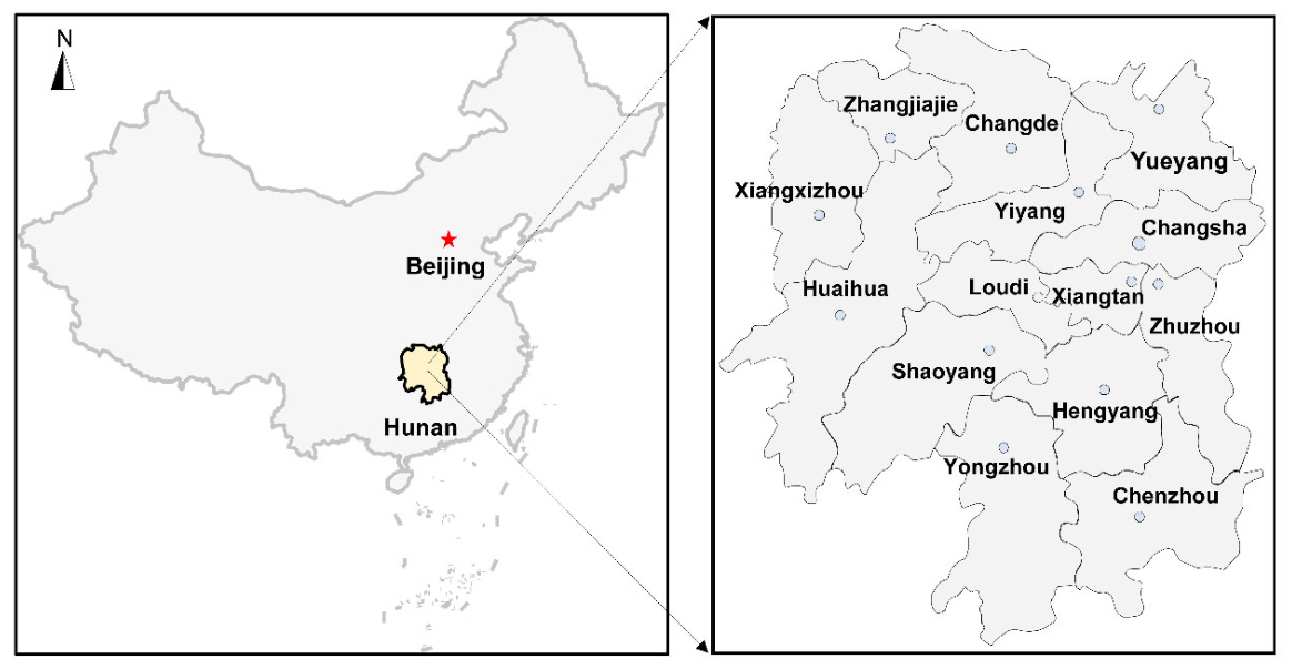
The study area is located in Hunan Province (108°47′–114°15′ E, 24°39′–30°08′ N), situated in southern central China. This region serves as a strategic hinterland connecting China’s coastal southeastern regions with inland areas (Figure 1). In this study, 6 selected air quality parameters, including particulate matter (PM) with diameters less than 2.5 μm (PM2.5), PM with diameters less than 10 μm (PM10), sulfur dioxide (SO2), nitrogen dioxide (NO2), ozone (O3) and carbon monoxide (CO) were selected to describe the air quality in Hunan Province. The air pollutants were analyzed using the ambient air quality standards recommended by the Ministry of Ecology and Environment of the People’s Republic of China (GB 3095-2012) [22]. The water quality dataset includes 9 indicators: water temperature (WT), pH, dissolved oxygen (DO), permanganate index (CODMn), ammonia nitrogen (NH3-N), total phosphorus (TP), total nitrogen (TN), electrical conductivity (EC), and turbidity (TU), which were monitored in accordance with the requirements of the Environmental Quality Standards for Surface Water (GB3838-2002) [23]. Water and air quality data were obtained from municipal monitoring stations across Hunan Province between 2020–2024, sourced from the China National Environmental Monitoring Center (CNEMC; https://www.cnemc.cn), accessed on 10 August 2025. The monitored cities comprised Changsha, Zhuzhou, Xiangtan, Hengyang, Shaoyang, Yueyang, Changde, Zhangjiajie, Yiyang, Chenzhou, Yongzhou, Huaihua, Loudi, and Xiangxizhou. A total of 70 surface water quality monitoring stations (SWQMS) across 14 cities in Hunan Province were included in this study (Table S1). Four-hourly measurements from each SWQMS were aggregated into monthly averages. For air quality, 82 monitoring stations were used, with hourly data averaged to derive the monthly concentrations.

2.2. Annual Trend Analysis

We employed a rigorous nonparametric statistical framework to quantify the temporal trends in 15 air and water quality parameters across Hunan Province from 2020 to 2024, accounting for key characteristics of environmental monitoring data including non-normal distributions, seasonal variations, and potential outliers. Initial seasonal pattern detection was performed using autocorrelation function (ACF) analysis with a 12-month lag window. The 95% confidence interval for the autocorrelation coefficient was calculated using Bartlett’s approximation [24]. A parameter was considered to exhibit potential seasonality if |ACF12| exceeded this critical value (p < 0.05). Parameters that met this criterion subsequently underwent seasonal and trend decomposition using loess (STL) decomposition to isolate underlying trends from seasonal components [25]. For trend assessment, we applied the robust Mann–Kendall (MK) test (α = 0.05) to evaluate monotonic patterns while avoiding distributional assumptions [26,27], with trend magnitudes quantified using Sen’s slope estimator (95% CIs) to provide outlier-resistant estimates of change rates [28]. All analyses were conducted in R software (v 2025.05.1) using the trend and forecast packages (v 9.0.2) [29,30].

2.3. Principal Component Analysis (PCA)

PCA was conducted to examine the relationships between atmospheric and aquatic parameters using R software with FactoMineR package (v 2.14) following the established dimensionality reduction protocols [31]. Prior to analysis, the dataset underwent rigorous preprocessing, including pairwise deletion of missing values (<1% of observations) [32] and standardization (z-score transformation) to ensure comparability across measurement scales [33]. The PCA implementation employed singular value decomposition with component retention determined by eigenvalues > 1 (Kaiser criterion) [34].

2.4. Spearman Rank Correlation Analysis

Prior to conducting Spearman rank correlation analysis, we implemented pairwise deletion to handle missing values, preserving maximal data integrity while minimizing bias in subsequent analyses. Correlation matrices were computed using the Hmisc package (v 5.2-5) in R software [35], implementing Spearman’s ρ specifically chosen to accommodate potential non-linear relationships while maintaining robustness against non-normal data distributions. Parameters were systematically ordered by descending mean absolute correlation strength to reveal dominant environmental associations. Statistical significance was determined at threshold (p < 0.05) with false discovery rate adjustment via the Benjamini–Hochberg procedure [36].

2.5. Cross-Correlation Function (CCF) Analysis

To investigate potential time-lagged relationships between atmospheric pollutants and water quality parameters, we conducted CCF analyses following established time-series approaches [24,37]. Prior to analysis, each monthly time series was tested for stationarity using the Augmented Dickey–Fuller (ADF) test. To remove seasonal effects and residual autocorrelation, each stationary series was pre-whitened by fitting a seasonal ARIMA model (SARIMA) with period 12, and the residuals were verified as white noise using the Ljung–Box test (p > 0.05 for all lags). As a sensitivity check, seasonal adjustment was also performed using STL. Correlations were then computed in R using the forecast package across biologically relevant monthly lags of ±12 months [29]. Statistical significance was assessed at α = 0.05 following false discovery rate (FDR) correction for multiple comparisons.

3. Results

3.1. Statistical Summary of Monitoring Data

The statistical descriptions for all of the water and air quality parameters are shown in Table 1. Atmospheric PM exhibited the most pronounced fluctuations, with PM2.5 concentrations (12.54–80.94 μg/m3, Q50 = 33.03 μg/m3, CV = 46.9%) demonstrating greater variability than PM10 (22.83–108.60 μg/m3, Q50 = 49.51 μg/m3, CV = 38.6%). Gaseous pollutants showed distinct distribution patterns: SO2 (5.17–11 μg/m3, CV = 14.5%) and CO (0.50–1.01 mg/m3, CV = 17.3%) maintained relatively stable levels. However, O3 (30.85–112.03 μg/m3, CV = 25.05%) and NO2 (8.11–38.88 μg/m3, CV = 37.2%) exhibited strong heterogeneity. Water quality parameters showed differing degrees of variability, with physical parameters demonstrating particularly dynamic behavior. WT (9.06–31.76 °C, CV = 32.2%) and TU (12.70–71.44 NTU, CV = 47.4%) exhibited the most substantial variations, whereas EC (201.94–307.84 μS/cm, CV = 10.78%) remained relatively stable, reflecting more consistent ionic composition in the water column. Chemical parameters revealed significant nutrient imbalances, with TN (1.07–2.41 mg/L, Q50 = 1.70 mg/L) exceeding the TP concentrations (0.04–0.09 mg/L, Q50 = 0.05 mg/L) by approximately 34-fold at Q50 levels. NH3-N exhibited marked temporal variability (0.09 ± 0.03 mg/L, CV = 37.3%), with concentrations spanning an order of magnitude (0.01–0.16 mg/L). Meanwhile, CODMn (1.46–2.69 mg/L, CV= 14.7%) and DO (6.19–10.5 mg/L, CV= 13.64%) displayed intermediate variability. Notably, pH levels exhibited remarkably stable conditions with minimal variation (7.05–7.86, CV = 1.7%), demonstrating the lowest variability among all analyzed parameters.

3.2. Annual Trends of Water and Air Quality

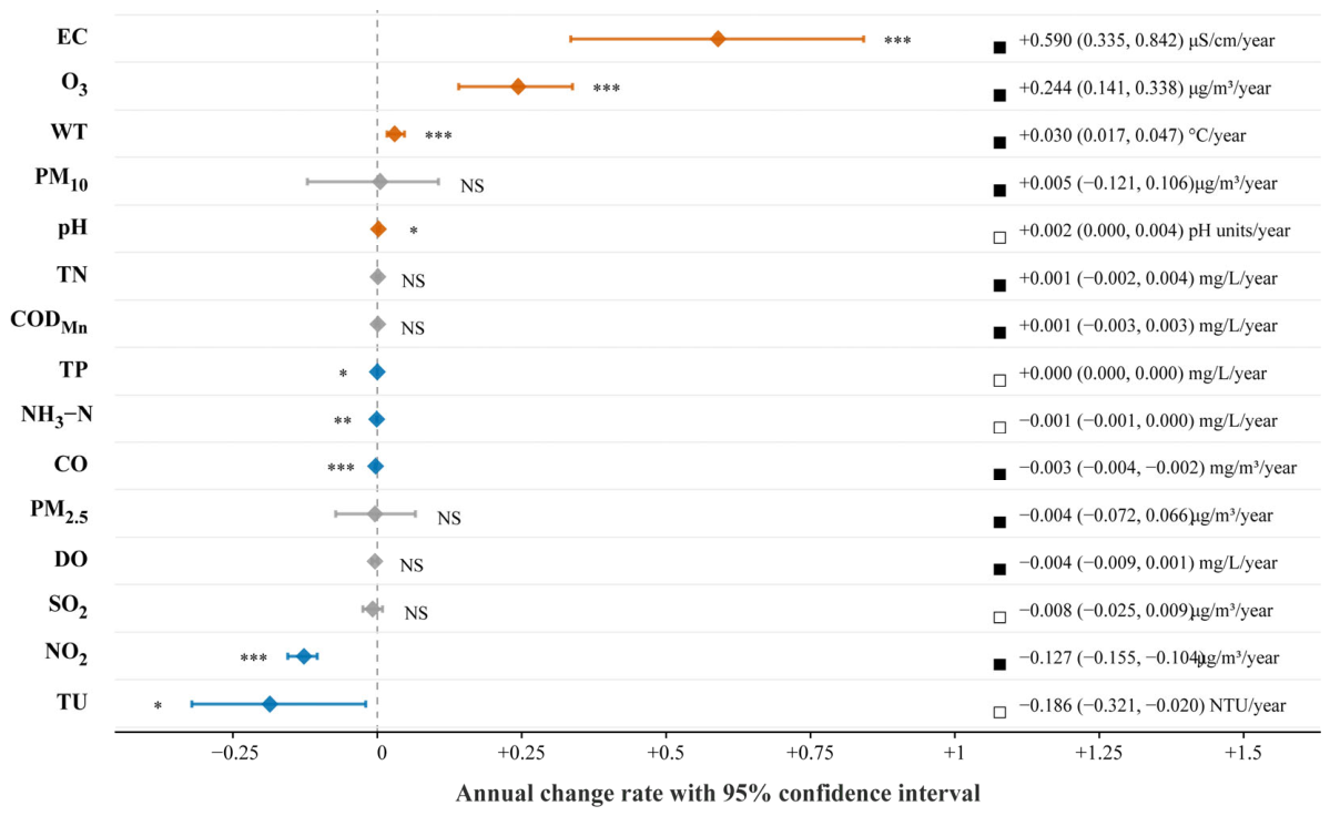
The temporal variations in water and air quality from 2020 to 2024 were assessed using the non-parametric MK and SS test (Figure 2). Prior to trend assessment, we conducted STL for all parameters to accurately identify and quantify seasonal components, ensuring that detected long-term trends were not confounded by periodic fluctuations. Analysis revealed that 10 parameters exhibited statistically significant seasonal variations (p < 0.05) including EC, O3, WT, PM10, TN, CODMn, PM2.5, CO, DO and NO2. For atmospheric pollutants, O3 showed the most pronounced increasing trend (+0.24 μg/m3/year, p < 0.001), while NO2 exhibited the steepest decline (−0.127 μg/m3/year, p < 0.001). In contrast, PM2.5, PM10 and SO2 showed no significant trends (p > 0.05). For water quality parameters, significant increases were detected in WT (+0.03 °C/yr, p < 0.001), pH (+0.002 /yr, p < 0.05), and EC (+0.59 μS/cm/yr, p < 0.001). Conversely, NH3-N, TP, and TU showed significant decreasing trends (−0.0008 mg/L/yr, −0.0002 mg/L/yr, and −0.19 NTU/yr, respectively; p < 0.05). DO, CODMn, and TN exhibited no statistically significant trends (p > 0.05).

3.3. Analysis of Water and Air Quality Correlations

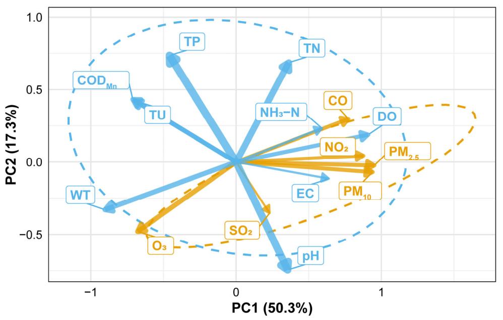
PCA was performed to explore the underlying relationships among the air and water quality parameters. The first two principal components (PC1 and PC2) had eigenvalues > 1 (7.54 and 2.60, respectively) and collectively explained 67.6% of the total variance (PC1: 50.3%, PC2: 17.3%; Table S3, Figure 3). PC1 was strongly dominated by atmospheric particulate matter and gaseous pollutants, with high positive loadings from PM2.5 (0.95), PM10 (0.94), NO2 (0.88), and CO (0.77). These four variables together contributed >40% of the variance explained by PC1 (Table S3). In addition, several water quality parameters associated with nutrient status, particularly TN (0.36) and NH3-N (0.59), exhibited positive loadings on PC1. These results indicate a non-negligible linkage between air quality and water quality in the atmosphere and environment, particularly regarding nitrogen species (TN and NH3-N).
PC2 was predominantly associated with the water quality parameters reflecting eutrophication and organic matter, with the highest loadings from pH (−0.74), TP (0.74), and TN (0.69). Moderate positive loadings were also observed for CODₘₙ (0.43), TU (0.42), and NH3-N (0.23).
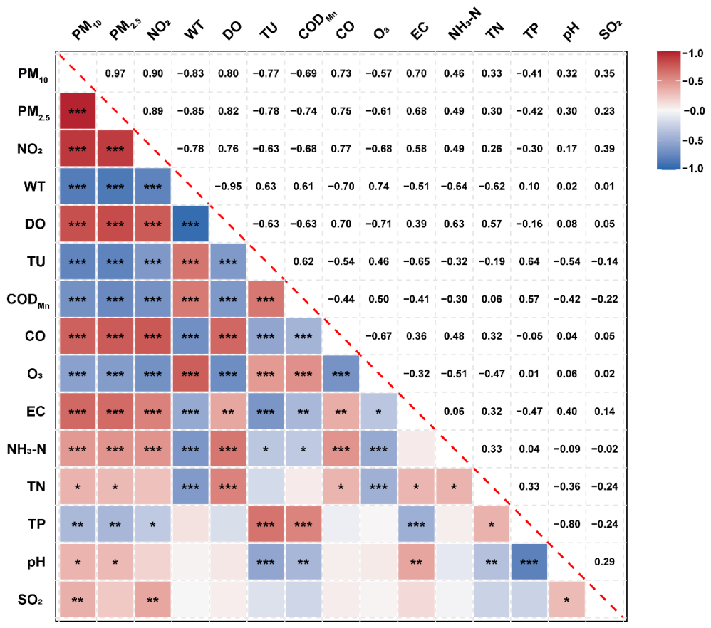
To further elucidate the relationships between atmospheric pollutants and water quality variables, we conducted Spearman’s rank correlation analysis (Figure 4). The results show that PM exhibited a strong positive correlation (ρ = 0.972, p < 0.001), suggesting that they may share common pollution sources and similar transmission mechanisms. In addition, PM pollutants were significantly positively correlated with NO2 and CO (p < 0.001), but significantly negatively correlated with O3 (p < 0.001). Regarding water quality impacts, PM pollutants were negatively correlated with TU, WT, TP, and CODMn (p < 0.05) but positively correlated with DO, NH3-N, and TN (p < 0.05). Gaseous pollutants (NO2, CO) were significantly positively correlated with DO, EC, and NH3-N (p < 0.05) and significantly negatively correlated with WT and TU (p < 0.001). O3 was significantly positively correlated with WT, TU, and CODMn (p < 0.001) and significantly negatively correlated with DO, TN, and NH3-N (p < 0.001).

3.4. CCF Analysis of Key Water Quality and Air Quality Indicators

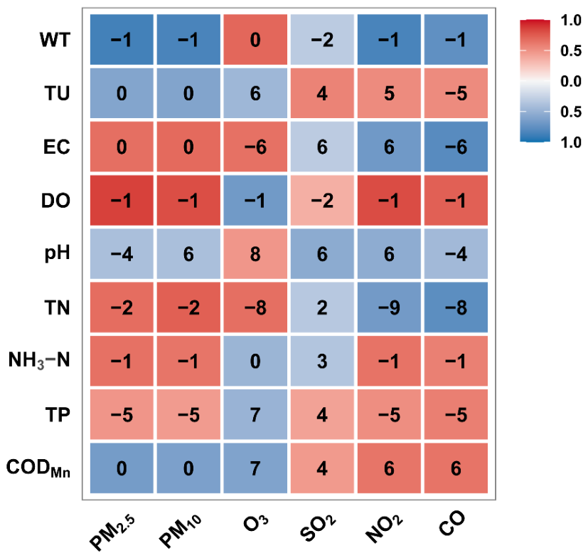
Cross-correlation function (CCF) analysis was employed to quantify the similarity between two time series and identify potential time-lagged or frequency-dependent relationships. In this study, the results revealed statistically significant (p < 0.05) monthly-scale associations between atmospheric pollutants and the water quality parameters (Figure 5). The magnitude of correlation coefficients ranged from moderate to very strong (|r| = 0.31–0.87), demonstrating distinct lag-phase responses critical for environmental regulation. PM2.5 exhibited strong negative correlations with WT (r = −0.87, lag −1) but positive associations with DO (r = 0.86, lag −1), TP (r = 0.48, lag −5), TN (r = 0.63, lag −2), and NH3-N (r = 0.65, lag −1). Similarly, PM10 correlated negatively with WT (r = −0.84, lag −1) and positively with DO (r = 0.81, lag −1), TP (r = 0.45, lag −5), NH3-N (r = 0.64, lag −1), and TN (r = 0.73, lag −2), suggesting PM as a potential nitrogen source through atmospheric deposition. These patterns suggest that PM may act as a potential N and P source in water. O3 was positively correlated with EC (r = 0.65, lag = −6) and TN (r = 0.67, lag = −8) and negatively correlated with TP (r = −0.49, lag = 7) and CODMn (r = −0.61, lag = 7). SO2 showed positive correlations with TU (r = 0.57, lag = 4), TP (r = 0.42, lag = 4), and CODMn (r = 0.46, lag = 4) but negative correlations with EC (r = −0.31, lag = 6), pH (r = −0.55, lag = 6), TN (r = −0.33, lag = 2), and NH3-N (r = −0.36, lag = 3). Both NO2 and CO exhibited highly consistent temporal lag effects, showing strong positive correlations with DO, NH3-N, TP, and CODMn. However, they demonstrated a negative lagged correlation with TN.

4. Discussion

Air and water pollutants exhibit dynamic interactions through physical transport, chemical transformation, and biological processes, creating complex feedback loops that amplify environmental risks in urbanizing regions [38]. Thus, comprehensive assessment of coupled atmospheric–aquatic systems is critical for understanding cross-ecosystem pollution dynamics.
Air pollutants that pose significant health risks include PM and oxides of various elements. Since the early 2000s, China has faced persistent air pollution challenges driven by rapid urbanization and industrial expansion [39]. In 2013, the hourly PM2.5 concentration in Beijing, China’s capital, even exceeded 680 μg/m3, which is 27 times higher than the World Health Organization (WHO) standard for good health [40]. However, the annual average PM2.5 concentration across 339 cities dropped to 29 μg/m3 in 2022, a 35.6% decrease from 2015 in China [41]. Our study findings indicate that during the 2020–2024 period, annual mean concentrations of PM2.5 and PM10 in Hunan Province reached 35.4 and 51.5 μg/m3, respectively, with no statistically significant decreasing trend observed. However, a comparative analysis showed that Hunan’s annual PM2.5 concentrations decreased from exceeding China’s official air quality standard (>35 μg/m3) during 2015–2016 to 35.4 μg/m3 in 2020–2024 [19], demonstrating measurable air quality improvement despite subsequent stabilization trends. During the study period, concentrations of NO2 and SO2 exhibited declining trends. Notably, NO2 also serves as a key precursor for O3 formation. Furthermore, nitrogen oxides (NOx) undergo complex atmospheric reactions with O3, yielding various hazardous secondary products including nitrate radicals and nitroaromatic compounds [42]. However, O3 concentrations exhibited a significant increasing trend during the same period. This inconsistent phenomenon of changes in NO2 and O3 has also been discovered in previous studies. During the COVID-19 pandemic, the emissions of NO2 in China decreased significantly, while the level of O3 increased significantly [43,44]. The mechanisms leading to this phenomenon are still under debate. Previous studies suggest that changes in O3 depend on various local factors, namely the levels of NOx, VOCs, oxidant levels, and meteorology [45].
Anthropogenic activities and natural environmental changes collectively influence water quality through multiple interacting pathways [46]. The observed reductions in NH3-N, TP, and TU strongly suggest the successful implementation of pollution mitigation measures, aligning with long-term water quality improvements across Hunan Province [21]. TU is frequently linked to heightened organic matter loads, as suspended sediments often transport decomposing particulate organic carbon and adsorbed nutrients (e.g., phosphorus, nitrogen). These organic–inorganic complexes can stimulate microbial activity, depleting DO. Furthermore, an increase in WT may facilitate the rapid growth of phytoplankton and filamentous algae, thereby increasing the risk of harmful algal blooms (HABs). Although algae produce oxygen through photosynthesis, their respiration during the night and the subsequent decomposition process of dead algae consume a large amount of DO. This ecological mechanism offers a possible interpretation for the observed non-significant trend in DO. Notably, among all parameters, EC exhibited the most pronounced annual increase rate. EC is an important water quality parameter and is an indicator of ion concentration changes [47]. Previous studies have shown that wet deposition is closely related to the concentration of major ions including Na+, Ca2+, Cl, and SO42− [48]. In addition, other factors may also contribute to this situation, such as increased ion inputs from agriculture and urban drainage. Therefore, further targeted research is needed to identify the main driving factors.
Atmospheric deposition is an important source of nutrients for both aquatic and terrestrial ecosystems. For example, global atmospheric nitrogen (N) deposition increased from 31.6 to 195.0 Tg N yr−1, while in China, it rose from 13.2 to 21.0 kg N ha−1 yr−1 between the 1980s and 2000s [49]. In Lake Taihu, atmospheric inputs accounted for 13.9–27.3% of riverine N loading via NH4+ and NO3 deposition [50]. These water-soluble inorganic ions are not only an important component of PM but also influence the pH of rainwater [51]. Previous studies in North America and Europe have shown that reducing emissions of air pollutants can lead to an improvement in water quality [46,52]. Our analysis revealed significant positive correlations between PM and TN, NH3-N, EC, and pH. These findings indicate potential linkages between atmospheric pollutants and aquatic conditions.
However, although atmospheric pollutants exhibit significant correlations with water quality parameters, their impacts on ecosystem alterations fundamentally differ from those of point source pollution. While point sources induce immediate downstream water quality perturbations, atmospheric deposition mediates aquatic ecosystem changes through indirect, time-lagged pathways [53]. Consequently, rigorous quantification of these lagged responses is essential for accurately assessing the legacy effects of emission reduction policies. Our CCF results clarify the time-lagged interactions between air and water quality. The 1–5 month lags observed between PM, NO2, CO, and aquatic nutrients (NH3-N, TP) are consistent with the time required for atmospheric deposition to transport pollutants from the atmosphere to aquatic systems, undergo dissolution and transformation, and ultimately affect water quality indicators [54]. Specifically, PM showed positive correlations with NH3-N and TN at 1–2 month lags, while its correlation with TP occurred at a 5-month lag. This distinction may arise from their differential speciation in particulate matter: N predominantly occurs as soluble ionic species (e.g., NH4+, NO3), whereas P primarily exists bound to particulate matrices [55,56]. This differential lag pattern highlights the need to consider pollutant speciation when evaluating the ecological impacts of atmospheric deposition. Gaseous pollutants (NO2, CO) also exhibited significant time-lagged correlations with aquatic nutrients, further supporting the role of atmospheric deposition in nutrient cycling. NO2, a precursor to nitric acid (HNO3) and nitrate aerosols, contributes to nitrogen deposition through both dry and wet pathways [42]. The observed 1–5 month lags between NO2 and NH3-N/TN may reflect the time required for NO2 to undergo atmospheric oxidation to NO3, followed by deposition and subsequent transformation to NH4+ via microbial nitrification–denitrification processes in water. Although CO is not a direct nutrient source, it serves as an effective tracer of incomplete combustion processes (e.g., fossil fuel and biomass burning). The significant positive correlations between CO and aquatic nutrients (NH3-N, TP) at lags of 1–5 months thus suggest a statistical co-occurrence between combustion-related emissions and aquatic nutrient enrichment. These findings strengthen the conceptual linkage between anthropogenic combustion activities and aquatic eutrophication pathways.
This study also has several limitations that should be acknowledged. First, the analysis relies on monitoring station data, which may not fully capture the spatial heterogeneity of air and water quality in rural and remote areas of Hunan Province. Future studies should incorporate more monitoring sites in these regions to improve spatial representativeness. Second, we did not consider the influence of land use types (e.g., urbanization, agriculture, forestry) on air–water interactions, which may mediate the deposition and transformation of pollutants. Integrating land use data into future analyses could provide deeper insights into the drivers of cross-media pollution. Third, controlled experiments or mechanistic models are needed to verify the causal links between atmospheric pollutants and water quality changes observed in this study.

5. Conclusions

In conclusion, our study systematically investigates the synergistic relationship between air and water quality in Hunan Province from 2020 to 2024, revealing significant temporal trends and complex cross-media interactions. The key findings include the stabilization of PM concentrations, increasing O3 and decreasing NO2 in air; improving water quality (reduced NH3-N, TP, TU) alongside rising EC, WT, and pH; and significant time-lagged correlations between atmospheric pollutants and aquatic nutrients, indicating that atmospheric deposition may serve as a contributing pathway for cross-media pollution. These findings highlight the need for integrated environmental management strategies that consider the interconnectedness of air and water systems, particularly in regional contexts similar to Hunan Province.

Supplementary Materials

The following supporting information can be downloaded at: https://www.mdpi.com/article/10.3390/atmos17060545/s1, Table S1: Geographic coordinates of surface water quality monitoring sections in Hunan Province, China; Table S2: Geographic coordinates of air quality monitoring sections in Hunan Province, China; Table S3: Loadings and contributions of each parameter to PC1 and PC2.

Author Contributions

Conceptualization, W.Z., Y.T. and Q.T.; methodology, X.C., T.F. and Y.W.; software, B.A., D.Y. and D.Y.; formal analysis, R.G., Y.H. and S.L.; writing—original draft preparation, W.Z., Y.T. and Q.T.; writing—review and editing, W.Z.; supervision, W.Z. All authors have read and agreed to the published version of the manuscript.

Funding

This study was jointly supported by the Scientific Research Fund of Hunan Provincial Education Department (25B0764), the Chenzhou National Sustainable Development Agenda Innovation Demonstration Areas Construction Provincial Special Funding (2022sfq51), and the Research Fund of Xiangnan University (2023[30]).

Data Availability Statement

The data that support the findings of this study are available from the corresponding author upon reasonable request.

Acknowledgments

We thank Feiran Wang for his valuable guidance on the statistical analysis of this study.

Conflicts of Interest

The authors declare no conflicts of interest.

References

  1. Cohen, A.J.; Brauer, M.; Burnett, R.; Anderson, H.R.; Frostad, J.; Estep, K.; Balakrishnan, K.; Brunekreef, B.; Dandona, L.; Dandona, R.; et al. Estimates and 25-year trends of the global burden of disease attributable to ambient air pollution: An analysis of data from the Global Burden of Diseases Study 2015. Lancet 2017, 389, 1907–1918. [Google Scholar] [CrossRef]
  2. Liu, M.; Li, W.; Yang, G.; Wang, X. Breathing and breeding: How air pollution shapes fertility intentions in China. Environ. Impact Assess. Rev. 2026, 116, 108114. [Google Scholar] [CrossRef]
  3. Nakyai, T.; Santasnachok, M.; Thetkathuek, A.; Phatrabuddha, N. Influence of meteorological factors on air pollution and health risks: A comparative analysis of industrial and urban areas in Chonburi Province, Thailand. Environ. Adv. 2025, 19, 100608. [Google Scholar] [CrossRef]
  4. Matus, K.; Nam, K.-M.; Selin, N.E.; Lamsal, L.N.; Reilly, J.M.; Paltsev, S. Health damages from air pollution in China. Glob. Environ. Change 2012, 22, 55–66. [Google Scholar] [CrossRef]
  5. Wang, F.; Hua, K.; Tian, Y.; Wei, M.; Xia, X.; Wang, L.; Feng, Y.; Li, X. Association between ambient air pollution and ischemic stroke hospitalization: A multicenter case-crossover study in Tianjin, China. Atmos. Environ. 2025, 360, 121400. [Google Scholar] [CrossRef]
  6. Zhang, T.; Yan, R.; Zhang, X.; Ni, J.; Fang, L.; Zhao, H.; Ma, Y.; Liu, S.; Pan, F. Association between ambient air pollution and cardiovascular disease mortality: An individual-level case-crossover study in Hefei, China. Ecotoxicol. Environ. Saf. 2025, 302, 118632. [Google Scholar] [CrossRef]
  7. McGrath, J.M.; Betzelberger, A.M.; Wang, S.; Shook, E.; Zhu, X.-G.; Long, S.P.; Ainsworth, E.A. An analysis of ozone damage to historical maize and soybean yields in the United States. Proc. Natl. Acad. Sci. USA 2015, 112, 14390–14395. [Google Scholar] [CrossRef] [PubMed]
  8. Lin, L.; Yang, H.; Xu, X. Effects of Water Pollution on Human Health and Disease Heterogeneity: A Review. Front. Environ. Sci. 2022, 10, 880246. [Google Scholar] [CrossRef]
  9. Nguyen, X.T.; Le, T.T.; Nguyen, K.H.; Nguyen, T.T.T.; Luu, T.P.K. Assessing air pollution and seasonal variations in Dong Nai Province, Vietnam: A geospatial analysis of key air quality parameters (2022−2023). Urban Clim. 2025, 61, 102475. [Google Scholar] [CrossRef]
  10. Liu, T.; Chan, A.W.H.; Abbatt, J.P.D. Multiphase Oxidation of Sulfur Dioxide in Aerosol Particles: Implications for Sulfate Formation in Polluted Environments. Environ. Sci. Technol. 2021, 55, 4227–4242. [Google Scholar] [CrossRef]
  11. Stein, A.F.; Lamb, D. Chemical indicators of sulfate sensitivity to nitrogen oxides and volatile organic compounds. J. Geophys. Res. Atmos. 2002, 107, ACH 13-1–ACH 13-11. [Google Scholar] [CrossRef]
  12. Nguyen, G.T.H.; La, L.T.; Hoang-Cong, H.; Le, A.H. An exploration of meteorological effects on PM(2.5) air quality in several provinces and cities in Vietnam. J. Environ. Sci. 2024, 145, 139–151. [Google Scholar] [CrossRef]
  13. Anderson, K.A.; Downing, J.A. Dry and wet atmospheric deposition of nitrogen, phosphorus and silicon in an agricultural region. Water Air Soil Pollut. 2006, 176, 351–374. [Google Scholar] [CrossRef]
  14. Brahney, J.; Hallerud, M.; Heim, E.; Hahnenberger, M.; Sukumaran, S. Plastic rain in protected areas of the United States. Science 2020, 368, 1257–1260. [Google Scholar] [CrossRef]
  15. Zhai, S.; Yang, L.; Hu, W. Observations of atmospheric nitrogen and phosphorus deposition during the period of algal bloom formation in northern Lake Taihu, China. Environ. Manag. 2009, 44, 542–551. [Google Scholar] [CrossRef] [PubMed]
  16. Chien, C.-T.; Allen, B.; Dimova, N.T.; Yang, J.; Reuter, J.; Schladow, G.; Paytan, A. Evaluation of atmospheric dry deposition as a source of nutrients and trace metals to Lake Tahoe. Chem. Geol. 2019, 511, 178–189. [Google Scholar] [CrossRef]
  17. Burton, A.; Aherne, J.; Hassan, N. Trace metals in upland headwater lakes in Ireland. Ambio 2013, 42, 702–714. [Google Scholar] [CrossRef]
  18. Yadav, R.; Pandey, P. A Review on Volatile Organic Compounds (VOCs) as Environmental Pollutants: Fate and Distribution. Int. J. Plant Environ. 2018, 4, 14–26. [Google Scholar] [CrossRef]
  19. Dai, C.; Huang, S.; Peng, H.; Yi, K.; Zhou, Y.; Qin, P. Particulate pollution status and its characteristics during 2015–2016 in Hunan, China. Atmos. Pollut. Res. 2019, 10, 739–748. [Google Scholar] [CrossRef]
  20. Xu, Z.; Mu, S.; Geng, X.; Liu, Y. Analysis of PM 2.5 Pollution Characteristics in Hunan Province Based on Wavelet Transform. Environ. Sci. Technol. 2024, 47, 80–92. [Google Scholar]
  21. Zhou, E.; Xue, C.; Zhang, J.; Song, L.; Xiao, K.; Cai, Z. Multi-model-driven analysis of temporal and spatial variation of water quality in Xiangjiang River. J. Phys. Conf. Ser. 2025, 2969, 012002. [Google Scholar] [CrossRef]
  22. GB 3095-2012; Ambient Air Quality Standards. China Environmental Science Press: Beijing, China, 2012.
  23. GB 3838-2002; Environmental Quality Standards for Surface Water. China Environmental Science Press: Beijing, China, 2002.
  24. Box, G.E.; Jenkins, G.M.; Reinsel, G.C.; Ljung, G.M. Time Series Analysis: Forecasting and Control; John Wiley & Sons: Hoboken, NJ, USA, 2015. [Google Scholar]
  25. Helsel, D.R.; Hirsch, R.M. Statistical Methods in Water Resources; Elsevier: Amsterdam, The Netherlands, 1993; Volume 49. [Google Scholar]
  26. Kendall, M.G. Rank Correlation Methods; Charles Griffen & Company: London, UK, 1948. [Google Scholar]
  27. Mann, H.B. Nonparametric tests against trend. Econometrica 1945, 13, 245–259. [Google Scholar] [CrossRef]
  28. Sen, P.K. Estimates of the regression coefficient based on Kendall’s tau. J. Am. Stat. Assoc. 1968, 63, 1379–1389. [Google Scholar] [CrossRef]
  29. Hyndman, R.J.; Khandakar, Y. Automatic time series forecasting: The forecast package for R. J. Stat. Softw. 2008, 27, 1–22. [Google Scholar] [CrossRef]
  30. Pohlert, T.; Pohlert, M.T.; Kendall, S. Package ‘Trend’: Non-Parametric Trend Tests and Change-Point Detection; R Foundation for Statistical Computing: Vienna, Austria, 2016. [Google Scholar]
  31. Lê, S.; Josse, J.; Husson, F. FactoMineR: AnRPackage for Multivariate Analysis. J. Stat. Softw. 2008, 25, 1–18. [Google Scholar] [CrossRef]
  32. Jolliffe, I.T.; Cadima, J. Principal component analysis: A review and recent developments. Philos. Trans. R. Soc. A 2016, 374, 20150202. [Google Scholar] [CrossRef]
  33. Legendre, P.; Legendre, L. Numerical Ecology; Elsevier: Amsterdam, The Netherlands, 2012; Volume 24. [Google Scholar]
  34. Peres-Neto, P.R.; Jackson, D.A.; Somers, K.M. How many principal components? Stopping rules for determining the number of non-trivial axes revisited. Comput. Stat. Data Anal. 2005, 49, 974–997. [Google Scholar] [CrossRef]
  35. Harrell, F.E., Jr.; Dupont, C. Hmisc: Harrell Miscellaneous, R package version 4; R Foundation for Statistical Computing: Vienna, Austria, 2020. [Google Scholar]
  36. Benjamini, Y.; Hochberg, Y. Controlling the false discovery rate: A practical and powerful approach to multiple testing. J. R. Stat. Soc. Ser. B 1995, 57, 289–300. [Google Scholar] [CrossRef]
  37. Fan, L.; Wang, Y.; Cao, C.; Chen, W. Teleconnections of Atmospheric Circulations to Meteorological Drought in the Lancang-Mekong River Basin. Atmosphere 2024, 15, 89. [Google Scholar] [CrossRef]
  38. Jiang, J.; Zhang, L.; Wang, Z.; Gu, W.; Yang, C.; Shen, Y.; Zhao, J.; Han, W.; Hu, Y.; Xue, F.; et al. Spatial consistency of co-exposure to air and surface water pollution and cancer in China. Nat. Commun. 2024, 15, 7813. [Google Scholar] [CrossRef]
  39. WHO Organization. WHO Global Air Quality Guidelines: Particulate Matter (PM2. 5 and PM10), Ozone, Nitrogen Dioxide, Sulfur Dioxide and Carbon Monoxide; WHO: Geneva, Switzerland, 2021. [Google Scholar]
  40. Wang, Y.; Yao, L.; Wang, L.; Liu, Z.; Ji, D.; Tang, G.; Zhang, J.; Sun, Y.; Hu, B.; Xin, J. Mechanism for the formation of the January 2013 heavy haze pollution episode over central and eastern China. Sci. China Earth Sci. 2013, 57, 14–25. [Google Scholar] [CrossRef]
  41. Gong, J.; Yin, Z.; Lei, Y.; Lu, X.; Zhang, Q.; Cai, C.; Chai, Q.; Chen, H.; Chen, R.; Chen, W.; et al. The 2023 report of the synergetic roadmap on carbon neutrality and clean air for China: Carbon reduction, pollution mitigation, greening, and growth. Environ. Sci. Ecotechnol. 2025, 23, 100517. [Google Scholar] [CrossRef] [PubMed]
  42. Li, Y.; Ye, C.; Ma, X.; Tan, Z.; Yang, X.; Zhai, T.; Liu, Y.; Lu, K.; Zhang, Y. Radical chemistry and VOCs-NO(x)-O(3)-nitrate sensitivity in the polluted atmosphere of a suburban site in the North China Plain. Sci. Total Environ. 2024, 947, 174405. [Google Scholar] [CrossRef]
  43. Zhao, Y.; Zhang, K.; Xu, X.; Shen, H.; Zhu, X.; Zhang, Y.; Hu, Y.; Shen, G. Substantial Changes in Nitrate Oxide and Ozone after Excluding Meteorological Impacts during the COVID-19 Outbreak in Mainland China. Environ. Sci. Technol. Lett. 2020, 7, 402–408. [Google Scholar] [CrossRef] [PubMed]
  44. Wang, H.; Huang, C.; Tao, W.; Gao, Y.; Wang, S.; Jing, S.; Wang, W.; Yan, R.; Wang, Q.; An, J.; et al. Seasonality and reduced nitric oxide titration dominated ozone increase during COVID-19 lockdown in eastern China. npj Clim. Atmos. Sci. 2022, 5, 24. [Google Scholar] [CrossRef]
  45. Kroll, J.H.; Heald, C.L.; Cappa, C.D.; Farmer, D.K.; Fry, J.L.; Murphy, J.G.; Steiner, A.L. The complex chemical effects of COVID-19 shutdowns on air quality. Nat. Chem. 2020, 12, 777–779. [Google Scholar] [CrossRef]
  46. Vorosmarty, C.J.; McIntyre, P.B.; Gessner, M.O.; Dudgeon, D.; Prusevich, A.; Green, P.; Glidden, S.; Bunn, S.E.; Sullivan, C.A.; Liermann, C.R.; et al. Global threats to human water security and river biodiversity. Nature 2010, 467, 555–561. [Google Scholar] [CrossRef]
  47. Marandi, A.; Polikarpus, M.; Jõeleht, A. A new approach for describing the relationship between electrical conductivity and major anion concentration in natural waters. Appl. Geochem. 2013, 38, 103–109. [Google Scholar] [CrossRef]
  48. Tsai, Y.I.; Hsieh, L.-Y.; Kuo, S.-C.; Chen, C.-L.; Wu, P.-L. Seasonal and rainfall-type variations in inorganic ions and dicarboxylic acids and acidity of wet deposition samples collected from subtropical East Asia. Atmos. Environ. 2011, 45, 3535–3547. [Google Scholar] [CrossRef]
  49. Galloway, J.N.; Dentener, F.J.; Capone, D.G.; Boyer, E.W.; Howarth, R.W.; Seitzinger, S.P.; Asner, G.P.; Cleveland, C.C.; Green, P.A.; Holland, E.A.; et al. Nitrogen Cycles: Past, Present, and Future. Biogeochemistry 2004, 70, 153–226. [Google Scholar] [CrossRef]
  50. Deng, J.; Nie, W.; Huang, X.; Ding, A.; Qin, B.; Fu, C. Atmospheric Reactive Nitrogen Deposition from 2010 to 2021 in Lake Taihu and the Effects on Phytoplankton. Environ. Sci. Technol. 2023, 57, 8075–8084. [Google Scholar] [CrossRef]
  51. Guo, W.; Long, C.; Zhang, Z.; Zheng, N.; Xiao, H.; Xiao, H. Seasonal Control of Water-Soluble Inorganic Ions in PM2.5 from Nanning, a Subtropical Monsoon Climate City in Southwestern China. Atmosphere 2019, 11, 5. [Google Scholar] [CrossRef]
  52. Ibarra-Morales, D.; Silva-Aguilera, R.A.; Oseguera, L.A.; Merino-Ibarra, M.; Alcocer, J. Impacts of global change on two tropical, high mountain lakes in Central Mexico. Sci. Total Environ. 2022, 852, 158521. [Google Scholar] [CrossRef] [PubMed]
  53. Feng, S.; Wang, M.; Heal, M.R.; Liu, X.; Liu, X.; Zhao, Y.; Strokal, M.; Kroeze, C.; Zhang, F.; Xu, W. The impact of emissions controls on atmospheric nitrogen inputs to Chinese river basins highlights the urgency of ammonia abatement. Sci. Adv. 2024, 10, eadp2558. [Google Scholar] [CrossRef]
  54. Nong, X.; Luo, K.; Lin, M.; Chen, L.; Long, D. Relationships between water quality of a long-distance inter-basin water diversion project and air pollution emissions along the canal: Distributions, lag effects, and nonlinear responses. Environ. Pollut. 2024, 361, 124813. [Google Scholar] [CrossRef]
  55. O’Day, P.A.; Nwosu, U.G.; Barnes, M.E.; Hart, S.C.; Berhe, A.A.; Christensen, J.N.; Williams, K.H. Phosphorus Speciation in Atmospherically Deposited Particulate Matter and Implications for Terrestrial Ecosystem Productivity. Environ. Sci. Technol. 2020, 54, 4984–4994. [Google Scholar] [CrossRef]
  56. Zhang, J.; Cheng, H.; Wang, D.; Zhu, Y.; Yang, C.; Shen, Y.; Yu, J.; Li, Y.; Xu, S.; Zhang, S.; et al. Chronic Exposure to PM(2.5) Nitrate, Sulfate, and Ammonium Causes Respiratory System Impairments in Mice. Environ. Sci. Technol. 2021, 55, 3081–3090. [Google Scholar] [CrossRef]
Figure 1. Spatial distribution of the study site.
Atmosphere 17 00545 g001
Figure 2. Forest plot displaying the annual change rates with 95% confidence intervals for all measured parameters. Filled squares denote parameters with significant seasonal patterns. Statistical significance: * p < 0.05, ** p < 0.01, *** p < 0.001. Symbols: ■ Seasonal pattern, □ No seasonal pattern, NS = Not significant.
Atmosphere 17 00545 g002
Figure 3. PCA variable factor map. Variables are colored by group (orange: atmospheric; blue: water quality). Arrow thickness reflects their relative contribution. Arrow length indicates the loadings of each variable to the principal components.
Atmosphere 17 00545 g003
Figure 4. Correlation heatmap of atmospheric pollutants and water quality parameters. Parameters are ordered hierarchically by continuous color gradient (blue–white–red), with significant correlations annotated (* p < 0.05, ** p < 0.01, *** p < 0.001). Numerical values show Spearman’s rank coefficients.
Atmosphere 17 00545 g004
Figure 5. Cross-correlation function (CCF) analysis between atmospheric pollutants and the water quality parameters. Blue (−1) to red (+1) indicates direction and strength of correlation (white = 0). Numerals represent the lag (in months) at which maximum absolute correlation occurs. Lag < 0 suggests that atmospheric precursors influence water quality. Lag > 0 implies that water conditions affect subsequent atmospheric composition.
Atmosphere 17 00545 g005
Table 1. Statistical summary of ambient air and water quality parameters.
ParametersUnitMean ± SD aMax bMin cQ25 dQ50 eQ70 fCV g
PM2.5μg/m335.35 ± 16.5880.9412.5422.5733.0340.2846.89%
PM10μg/m351.5 ± 19.9108.622.8335.2949.515838.64%
O3μg/m358.52 ± 14.66112.0330.8547.1160.2765.2925.05%
SO2μg/m37.81 ± 1.13115.177.17.868.2314.52%
NO2μg/m319.16 ± 7.1238.888.1113.7518.5122.2237.16%
COmg/m30.71 ± 0.121.010.50.640.70.7517.34%
WT°C20.77 ± 6.6931.769.0614.3520.6725.1732.19%
pH 7.66 ± 0.137.867.057.597.687.721.71%
DOmg/L8.3 ± 1.1310.56.197.327.979.0313.64%
CODMnmg/L1.91 ± 0.282.691.461.691.882.0314.70%
NH3-Nmg/L0.09 ± 0.030.160.010.070.090.137.28%
TPmg/L0.06 ± 0.010.090.040.050.050.0619.44%
TNmg/L1.69 ± 0.292.411.071.521.71.8317.08%
ECμS/cm250.15 ± 26.95307.84201.94227.67246.51266.1510.78%
TUNTU26.95 ± 12.7771.4412.718.5723.3327.1547.38%
a Mean: Arithmetic average of all measurements; SD: Standard deviation; b Max: Maximum value in the dataset; c Min: Minimum value in the dataset; d Q25: 25th percentile (lower quartile), below which 25% of data fall; e Q50: 50th percentile (median), midpoint of the dataset; f Q70: 70th percentile, below which 70% of data fall; g CV: Coefficient of variation (SD/Mean × 100).
Disclaimer/Publisher’s Note: The statements, opinions and data contained in all publications are solely those of the individual author(s) and contributor(s) and not of MDPI and/or the editor(s). MDPI and/or the editor(s) disclaim responsibility for any injury to people or property resulting from any ideas, methods, instructions or products referred to in the content.