Article

Assessment of Vertical Wind Characteristics for Wind Energy Utilization and Carbon Emission Reduction

1
School of Soil and Water Conservation, Beijing Forestry University, Beijing 100083, China
2
Powerchina Beijing Engineering Corporation Limited, Beijing 100083, China
3
Huaneng Renewables Corporation Limited Mengxi Branch, Hohhot 010000, China
*
Author to whom correspondence should be addressed.
Atmosphere 2026, 17(1), 102; https://doi.org/10.3390/atmos17010102 (registering DOI)
Submission received: 11 December 2025 / Revised: 16 January 2026 / Accepted: 16 January 2026 / Published: 18 January 2026
(This article belongs to the Section Climatology)

Abstract

With the rapid advancement of clean energy, wind farm planning and construction are expanding worldwide, increasing the demand for accurate resource assessments. This study investigates the influence of vertical wind characteristics on wind farm siting and energy production, using measured meteorological data from the Hangjinqi wind farm. Results show that both mean wind speed increase substantially with altitude, indicating that upper layers provide richer and more stable wind resources. The estimated annual energy production of the site reaches 23,500 MWh, with capacity factors ranging from 35% to 42%, well above the national average. Seasonal and diurnal variations are evident: wind speeds strengthen during winter and spring, particularly at night, while turbulence intensity peaks in the daytime and decreases with height. Carbon dioxide (CO2) reduction also increases with hub height, with the most pronounced seasonal reductions in spring (3367.6–5041.1 tCO2, +49.7%) and winter (3215.7–5380.0 tCO2, +67.4%), equivalent to several thousand tons of standard coal per turbine annually. Optimal performance is observed at 100–140 m, demonstrating efficient utilization of mid- to high-altitude resources. Nevertheless, discrepancies in turbine performance at different hub heights suggest untapped potential at higher elevations. These findings highlight the importance of incorporating vertical wind characteristics into wind farm siting decisions, and support the deployment of turbines with tower heights ≥140 m alongside intelligent scheduling and forecasting strategies to maximize energy yield and economic benefits.

1. Introduction

The global community faces escalating environmental challenges and natural resource depletion, necessitating an accelerated transition from conventional fossil fuels to clean and renewable energy sources [1]. This shift is critical for achieving significant carbon emission reductions, mitigating climate change impacts, and fulfilling sustainable development objectives [2,3]. In this context, wind energy plays a vital role not only in supplying clean electricity but also in substantially reducing carbon dioxide emissions by replacing fossil fuel-based power generation. Among renewable alternatives, wind energy has become a pivotal and rapidly expanding global clean energy resource [4]. China’s wind power sector has demonstrated substantial growth in recent years, with its contribution to the national electricity generation mix increasing markedly [5]. Notably, wind power accounted for 10% of China’s total electricity production in 2024, positioning it as the nation’s third-largest electricity generation source [6]. The expansion of wind power capacity in China has resulted in measurable carbon dioxide mitigation, contributing significantly to national carbon neutrality targets [7].
Wind power development reduces dependence on fossil fuels, enhances energy security, and is vital for advancing carbon neutrality goals and fostering green economic growth [8]. Consequently, the rigorous scientific evaluation of wind energy resources and wind farm operational efficiency is indispensable for optimizing wind power utilization, guiding strategic energy planning, and promoting sustainable, resilient energy systems [9,10]. Integrating carbon mitigation considerations into resource assessment and turbine performance analysis ensures that wind energy deployment maximizes environmental benefits alongside economic returns [11].
Wind farm resource assessment and operational efficiency analysis have become major priorities in wind energy research, attracting extensive attention both domestically and internationally [9]. To support scientifically rational wind resource development, numerous studies have focused on key meteorological parameters. For instance, Fei et al. [12] analyzed monthly variations and correlations between global temperature and wind resources, highlighting temporal variability, while Lu et al. [13] quantified the contributions of environmental factors to wind characteristics in China over 2000–2019, providing insights into regional influences. Wang et al. [14] developed methods for ultra-short-term forecasting of wind power output using multiple meteorological factors. Offshore and regional assessments have been advanced by Elshafei et al. [15] through hybrid data fusion and numerical models, and by Zhu et al. [16], who explored optimal layout strategies for wind resource utilization in Tibet.
Wind power density studies include Arrieta-Prieto and Schell [17], who applied data-driven optimization for farm siting, Dayal et al. [18] in Fiji, and Liu et al. [19], who conducted a long-term tower measurement case study in Beijing. Air density effects have been addressed by Floors and Nielsen [20] using observational and reanalysis data, by Liang et al. [21] through deep neural network modeling, and by Ulazia et al. [22] for global seasonal variations. Vertical wind profiles, including wind shear and turbulence intensity, have been investigated by Jung and Schindler [23], Kim et al. [24], Juan et al. [25], and reviewed comprehensively by Murthy and Rahi [4]. Traditional statistical approaches, such as Weibull distribution modeling, have been applied by Jung et al. [26] and Dai et al. [27] to characterize wind speed variability across different regions.
To capture spatiotemporal variations in wind fields more accurately, integrated methodologies combining physical models [28] and numerical simulations [29] have been used to capture spatiotemporal variations in wind fields more accurately. The deployment of emerging technologies, such as meteorological towers [30], LiDAR measurements [31], numerical weather prediction (NWP) [4], and computational fluid dynamics (CFD) [32], has facilitated high-resolution, multi-height wind field assessment. These approaches have significantly improved understanding of complex-terrain and multiscale wind characteristics, providing essential data support for wind farm siting, layout optimization, and turbine design.
In addition, the analysis of wind farm operational efficiency has evolved beyond single indicators such as capacity factor [33] and utilization hours [34], toward multidimensional evaluation frameworks [35]. Contemporary research investigates not only turbine power curve fitting [36,37] and actual power output [2] but also power loss mechanisms [38], inter-turbine wake effects [39,40], and performance impacts of equipment failures [41]. Furthermore, intelligent dispatching, real-time monitoring, and forecasting technologies [42,43], have substantially improved dynamic operational management, enhancing wind resource utilization and maximizing economic returns [44,45].
As wind energy deployment increasingly targets higher altitudes, understanding vertical wind resource characteristics has become critical for maximizing turbine performance and CO2 mitigation potential [46]. Despite significant progress, detailed empirical studies are still needed to compare turbines of different hub heights, identify spatial wind patterns, and quantify the carbon reduction benefits of high-altitude wind energy [15]. Therefore, integrating long-term, high-precision observational data with advanced analytical methods is essential for systematically assessing elevated wind resources and their influence on turbine performance.
Although substantial progress has been made in wind resource assessment and wind farm performance studies, limitations remain in terms of data depth and application scenarios. Many existing studies focus on large-scale or offshore wind resources, whereas empirical analyses based on long-term, multi-height measurements within operating inland wind farms are relatively scarce. In addition, the influence of vertical wind speed variation on turbine performance is often discussed independently from its potential contribution to carbon dioxide reduction. As a result, the combined effects of hub height, wind resource characteristics, and carbon mitigation benefits have not yet been fully clarified. Based on long-term meteorological observations from the Hangjinqi wind farm, this study examines altitude-dependent wind characteristics and their implications for energy production, turbine operation, and CO2 emission reduction, providing practical support for turbine selection and wind farm optimization.

2. Materials and Methods

2.1. Data Sources

The Hangjin Banner Wind Farm is situated in Hangjin Banner, Ordos, south of the Kubuqi Desert within the Inner Mongolia Autonomous Region. Its geographical coordinates range from 108° E to 110° E longitude and 39° N to 41° N latitude, representing a location of significant strategic importance. The wind farm comprises 32 wind turbines, each equipped with a dedicated transformer unit, and is supported by a central 220 kV booster station. The total installed capacity is 200 MW, achieved using 32 high-capacity wind turbines rated at 6 MW each. The technical details are based on internal project documentation and field surveys. Additionally, the project includes an integrated energy storage system with a capacity of 60 MW/120 MWh, enhancing grid stability and energy dispatch flexibility. This configuration exemplifies a modern, large-scale wind power deployment that integrates renewable generation with energy storage infrastructure, contributing to regional energy security and sustainable development.
Meteorological data used in this study were obtained from a meteorological observation tower located within the wind farm boundary. The tower is situated at approximately 40°02′ north latitude and 108°05′ east longitude, at an elevation of around 1550 m above sea level. Wind speed was measured at six heights, 30, 50, 80, 100, 120, and 140 m, with two anemometers installed at each height—one facing due north and the other due south—facilitating high-resolution characterization of the wind field in both spatial and directional dimensions. The measurements were collected from 1 January 2020 to 20 December 2020, with a sampling frequency of 10 min. In addition to wind speed, the dataset also includes wind direction, air temperature, and air pressure. Due to systematic instrument errors, equipment malfunctions, and problems during data transmission or recording, erroneous measurements may occur and thus require correction. The criteria for identifying such errors are defined as follows [30]:
(1)
Removal of stagnant values: In the time series, if a measurement remains unchanged for a prolonged period, it usually indicates sensor malfunction, signal transmission failure, or operational faults of the instrument. These constant readings are defined as stagnant (or frozen) values. Data points that deviate from the stagnant value by more than 0.5 are identified, and the segment from the onset of the stagnant value up to the point immediately before the deviation is discarded.
(2)
Elimination of outliers: Based on historical climatic statistics of the study area, wind speeds greater than 50 m/s are considered unrealistic and directly excluded. For temperature data, acceptable ranges are defined by season: −23 to 25 °C (January–March), −5 to 45 °C (April–June), 0 to 50 °C (July–September), and −20 to 30 °C (October–December). Measurements falling outside these ranges are regarded as outliers and removed.
(3)
Temporal continuity control: For each data point, the difference between its value and the weighted average of the four consecutive neighboring points is calculated. If the difference exceeds the specified threshold (5 m/s for wind speed and 4 °C for temperature), the point is deemed discontinuous. Such values are replaced using the four-point central interpolation method, with the interpolated value computed from the weighted average.
(4)
Spatial continuity control: When outliers cannot be corrected using the four-point central interpolation method, the spatial continuity of the measurements is employed. Specifically, if valid data from other heights are available at the same time step, spline interpolation based on the surrounding height levels is applied to estimate and replace the missing or erroneous value.
Sensitivity analysis indicated that the removal of erroneous measurements and subsequent interpolation had a negligible impact on the wind statistics. As illustrated in Figure 1, the framework integrates input datasets, key processing steps, and output results to systematically assess and model urban wind resources.

2.2. Method

2.2.1. Multi-Level Wind Resource Characteristics and Model Fitting

Based on wind speed data collected from multi-altitude meteorological observation towers, rigorous quality control was first applied to the raw dataset to remove outliers and address missing values, thereby ensuring the integrity and reliability of the data [30]. Subsequently, statistical analyses were conducted on the hourly and monthly wind speed records to extract key characteristics of diurnal and seasonal variation [47]. By calculating the mean wind speed and examining its spatiotemporal distribution across different height levels, this study investigates the vertical gradient of wind speed and its seasonal differences. Furthermore, by integrating the vertical temperature differences derived from atmospheric profiles and variations in surface pressure, the analysis explores the influence of thermal structure and atmospheric stability on wind speed characteristics. The overall objective is to systematically reveal the variation patterns of wind speed across multiple temporal and vertical scales, thereby providing essential data support for the assessment of wind resource potential.
The generalized extreme value (GEV) distribution, gamma distribution, Gumbel distribution, and Weibull distribution were fitted to the wind speed and air density data at different heights [30,48]. The optimal distribution model was selected based on the Kolmogorov–Smirnov (K-S) goodness-of-fit test. This step provides a robust and high-precision statistical foundation for the evaluation of annual energy production (AEP), thereby enabling more accurate predictions of the power generation potential of wind farms under various operating conditions. The probability models for the different distributions are presented in Equations (1)–(4).
The probability density function (pdf) of the GEV distribution is given by Equation (1) [49].
f v = 1 σ 1 + ξ ( v μ σ ) 1 1 ξ exp 1 + ξ ( v μ σ ) 1 ξ
where μ is the location parameter, σ > 0 is the scale parameter, ξ is the shape parameter, and the condition 1 + ξ v μ σ > 0 must hold.
The pdf of the gamma distribution is shown in Equation (2) [50].
f v = v k 1 v θ θ k Γ k
where k > 0 is the shape parameter, θ is the scale parameter, and Γ α is the gamma function.
The pdf of the Gumbel distribution is given in Equation (3) [51].
f v = 1 β exp v μ β exp v μ β
where μ is the location parameter and β > 0 is the scale parameter.
The PDF of the Weibull distribution is presented in Equation (4) [52].
f v = k λ ( v λ ) k 1 exp ( v λ ) k
where k > 0 is the shape parameter and λ > 0 is the scale parameter.
In this study, the parameters of the fitted probability distributions were estimated using the maximum likelihood estimation (MLE) method, and the goodness of fit was evaluated using the Kolmogorov–Smirnov (K-S) test. The detailed formulas and methodological procedures are presented as follows:
For a parameter set θ  and a given dataset X = x 1 , x 2 , , x n , the likelihood function L θ X is defined as [19]:
θ X = P X θ = i = 1 n P x i θ  
The consistency between the observed samples of wind speed and air density and the different distribution models was evaluated using the one-sample Kolmogorov–Smirnov (K-S) test. The test statistic D is defined as [31]:
D = sup F n v F ( v )
where F n v is the ECDF of the sample, and F ( v )  is the CDF of the reference distribution. The null hypothesis H0 states that the sample is drawn from the reference distribution. The test provides a p value indicating the probability of observing a test statistic as extreme as, or more extreme than, the observed value under H0.

2.2.2. Operational Security Assessment

Based on multi-level meteorological observation data, statistical analysis methods were employed to systematically investigate the spatiotemporal variation characteristics of the wind shear coefficient (α) and turbulence intensity (TI), providing essential meteorological and dynamic parameters to support subsequent wind resource assessment and wind farm design.
The wind shear coefficient α is calculated using the logarithmic difference in wind speeds between adjacent height levels, reflecting the rate of change of wind speed with height [23,24]. The calculation formula is given as:
α = ln v 2 ln v 1 ln h 2 ln h 1
where v 1 and v 2 represent the average wind speeds at two height levels h 1 and h 2 , respectively.
Turbulence intensity (TI) is defined as the ratio of the standard deviation of wind speed to the mean wind speed [4,24,25]. The calculation formula is:
T I = σ v v ¯
where σ v is the standard deviation of the wind speed, and v ¯ is the mean wind speed over the corresponding time period.

2.2.3. Wind Farm Power and Capacity Evaluation

The spatiotemporal distribution characteristics of air density are of great significance for wind energy assessment. However, many studies still treat air density as a constant when evaluating wind energy potential, even though it directly influences wind power density and, consequently, the accuracy of wind turbine energy yield predictions [22,53]. The present analysis highlights the importance of incorporating both seasonal and diurnal variations in air density into wind resource assessments and power prediction models. Such consideration can improve the scientific rigor of assessments while enhancing the economic efficiency of wind farm operation and management. The air density can be calculated via Equation (9).
ρ h = P h R d · T h
where ρ h represents the air density at height h (kg/m3), T h denotes the temperature at altitude h (K), R d is the specific gas constant for dry air, and P h is the atmospheric pressure at altitude h (Pa)
The fitted wind speed distribution was combined with the power curves of the turbine models employed in the study area to convert the wind speed resource into corresponding power density, and subsequently estimate the annual available energy production, thereby enabling a comprehensive assessment of the regional wind energy potential [54]. The calculation of wind power density (WPD) is presented in Equation (10) and the calculation of annual energy production (AEP) is provided in Equation (11).
W P D h = 1 2 ρ h V h 3
where W P D h is the wind power density at height h (W/m2), ρ h denotes the air density (kg/m3), and V h denotes the wind speed (m/s).
A E P = 8760 h 0 P W ( V , ρ ) f ( V ) d V
where f ( V ) denotes the wind speed probability density, and P W ( V , ρ ) denotes the specific power curve of the wind turbine.
The capacity factor and power generation efficiency of the unit under existing operational strategies are evaluated across different seasons, time periods, and dominant wind directions. By conducting detailed analyses stratified by season, time, and prevailing wind patterns, the performance variations under varying meteorological conditions are quantitatively assessed, and potential optimization opportunities and operational constraints are identified. The resulting insights provide robust quantitative references for the development of more efficient scheduling strategies and scientifically informed maintenance plans, while also establishing a methodological framework for the optimization of operational strategies through the integration of meteorological and power forecasting models.
The capacity factor is the ratio of actual power generation to full load power generation, reflecting the utilization efficiency of wind turbines [33,55,56]:
C F = A E P P r a t e d · T
where P r a t e d is the rated power of the turbine, and T represents the total number of hours in a year.
The power utilization ratio of a wind turbine reflects its power generation efficiency under given wind speed conditions [34,57], usually defined as:
η = P a c t u a l P m a x
where P a c t u a l represents the actual electrical power output generated by the wind turbine under given wind speed conditions (measured or derived from the power curve), and P m a x denotes the turbine’s rated electrical power.

2.2.4. Estimation of Carbon Emission Reductions

From an environmental perspective, wind power projects serve as an effective means to displace carbon emissions produced by fossil fuel–based electricity generation, thereby substantially reducing the overall carbon footprint throughout the lifecycle of project. The wind resource condition is a crucial factor influencing the energy production performance of wind farms and consequently determines their potential for carbon reduction. To accurately evaluate the carbon mitigation capacity of wind power projects, it is essential to first obtain quarterly and annual power generation data, followed by calculations based on wind speed forecasts and power distribution models under time-varying wind conditions. Subsequently, by applying the regional grid emission factor, a quantitative relationship between power generation and carbon emissions can be established, enabling the precise estimation of the total carbon reduction achieved [58].
First, the wind speed is converted into instantaneous power output through the turbine-specific power curve P W ( V , ρ ) .
P t , h = P ( v t , h )
where t denotes the time step and h represents the measurement height.
Subsequently, the energy generation at each time step is calculated. Given a temporal resolution of 10 min, the energy produced during each interval can be expressed as:
E t , h = P t , h · t
Based on the grid emission factor E F , the electricity generated by wind power is converted into the corresponding amount of carbon emission reduction, representing the avoided emissions from conventional grid-based power generation.
R t , h = E t , h · E F
At a given height level h , the total carbon reduction is obtained by summing the emissions avoided across all time steps.
R h t o t a l = t = 1 T R t , h

3. Results and Discussion

3.1. Wind Speed Characteristics

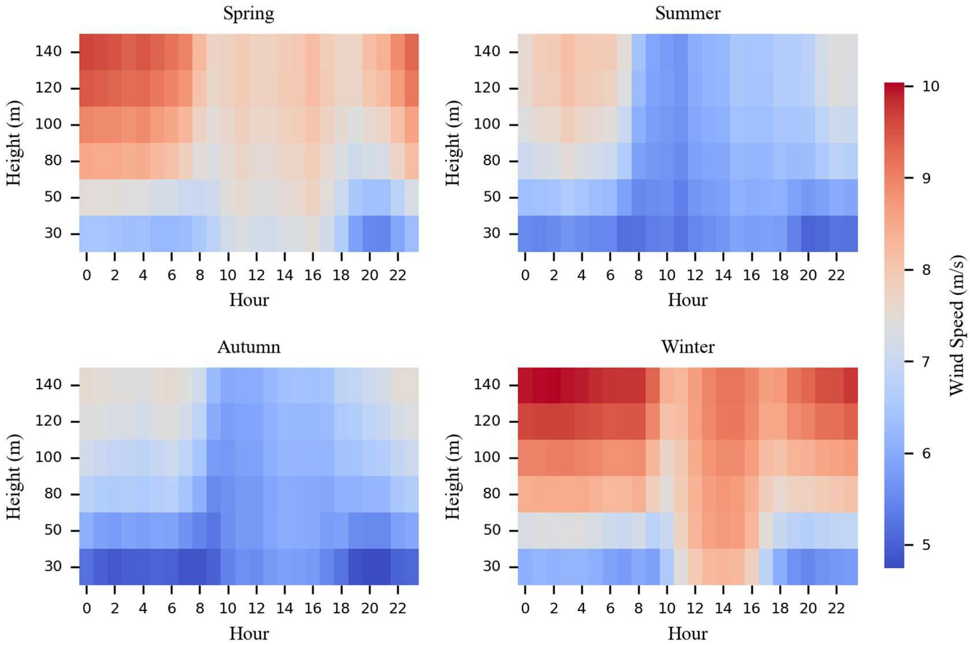
Figure 2 presents heatmaps of wind speed variation with height and hour across the four seasons. The results reveal a clear vertical gradient in all seasons, with wind speeds consistently increasing with height. This pattern aligns well with the classical boundary layer theory, which describes wind profiles following logarithmic or power-law scaling, primarily due to surface roughness damping the near-surface flow [59,60]. Distinct diurnal patterns emerge across the seasons. In spring and winter, nighttime (00:00–06:00, 18:00–24:00) wind speeds at higher altitudes are significantly stronger than during daytime, likely linked to enhanced nocturnal atmospheric stability and the occurrence of low-level jets [61,62]. In contrast, summer exhibits generally lower wind speeds with minimal diurnal variation, mainly governed by local thermal convection and lacking strong synoptic-scale forcing [63,64]. Autumn shows the most stable wind speed, with little difference between day and night, which may be attributed to transitional atmospheric stratification and background circulation during the season. Seasonal differences in average wind speed are also prominent. Winter demonstrates the highest overall wind speeds, with upper levels reaching 9–10 m/s, largely influenced by large-scale northwesterly flows and frequent cold air outbreaks [65]. Spring ranks second, characterized by strong seasonal winds, while summer records the lowest wind speeds, particularly near the surface, sometimes falling below 5 m/s. Autumn winds are slightly stronger than those in summer but remain weaker compared to the winter and spring seasons.
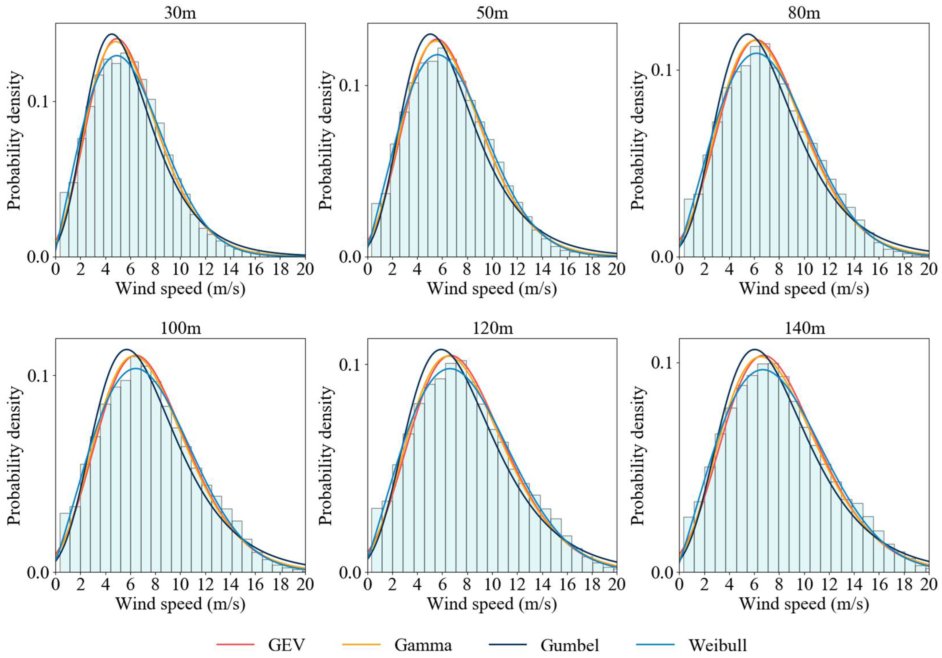
Figure 3 presents the annual wind speed probability density distributions across six height levels, from 30 m to 140 m, along with their fitting performance using various statistical distributions (GEV, Gamma, Gumbel, and Weibull). Across all height levels, the wind speed distributions exhibit right-skewed unimodal shapes, primarily concentrated between 4–10 m/s. Notably, at heights above 80 m, the peak probability density approaches 0.1, corresponding to the most frequent (modal) wind speeds of approximately 6–8 m/s. As altitude increases, the overall distribution shifts rightward, indicating an increasing probability of higher wind speeds and a declining proportion of low wind speeds. Table 1 summarizes the Kolmogorov–Smirnov (K-S) statistics for the goodness-of-fit of each distribution across the different heights. The results show that the Weibull distribution consistently yields the lowest K-S values at all height levels, indicating the closest match to the empirical wind speed distributions. This suggests that the Weibull model effectively captures both the central probability characteristics of medium-to-low wind speeds and the tail behavior at higher wind speeds. In contrast, the GEV and Gamma distributions provide moderately good fits, while the Gumbel distribution consistently shows the highest K-S values, reflecting weaker overall performance, particularly in the high wind speed range. In summary, the Weibull distribution not only demonstrates excellent visual alignment with the empirical distributions but also achieves superior statistical performance. Therefore, it is selected as the baseline model for subsequent wind energy resource calculations.

3.2. Vertical Wind Profile and Turbulence Analysis

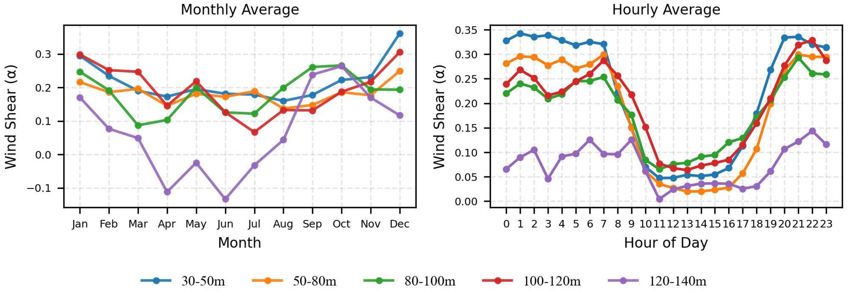
Figure 4 illustrates the diurnal variation in wind shear coefficients (α) across different height intervals (left) and the monthly variation in the average wind shear coefficient (α) across different height intervals (right). Overall, α values are generally lower during the daytime, especially around midday, showing a clear decreasing trend. This pattern reflects an unstable atmospheric boundary layer during the day, leading to reduced vertical wind shear. In contrast, wind shear coefficients increase significantly at night, peaking mostly during late night to early morning hours, indicating a stable atmospheric stratification that enhances wind speed increase with height [66,67]. Regarding vertical distribution, the lowest layer (30–50 m) consistently exhibits the highest α values, reaching night-time peaks around 0.33. Conversely, the uppermost layer (120–140 m) shows the lowest α values, with some daytime periods approaching zero or even negative values, suggesting a more uniform or occasionally inverted wind speed profile aloft. Intermediate layers (50–100 m) display α values between these extremes, with diurnal patterns similar in trend but smaller in magnitude. Overall, α values are relatively high during winter (December to February) and autumn (September to November), particularly in the 30–50 m and 100–120 m layers, indicating a pronounced increase in near-surface wind speed with height. In spring (March to May), α values remain moderate and wind speed vertical gradients are relatively stable. During summer (June to August), wind shear weakens significantly, especially in the upper layer (120–140 m), with some months exhibiting negative α values. This indicates a tendency toward a more homogeneous wind speed profile at higher altitudes, with occasional localized decreases in wind speed, which may be attributed to atmospheric instability and intensified convective processes [68]. Comparing different height intervals, wind shear coefficients in the lower to mid-levels (30–80 m) remain relatively stable year-round. In contrast, the upper layers (100–140 m) experience greater variability, strongly influenced by seasonal atmospheric processes and local dynamics [67].
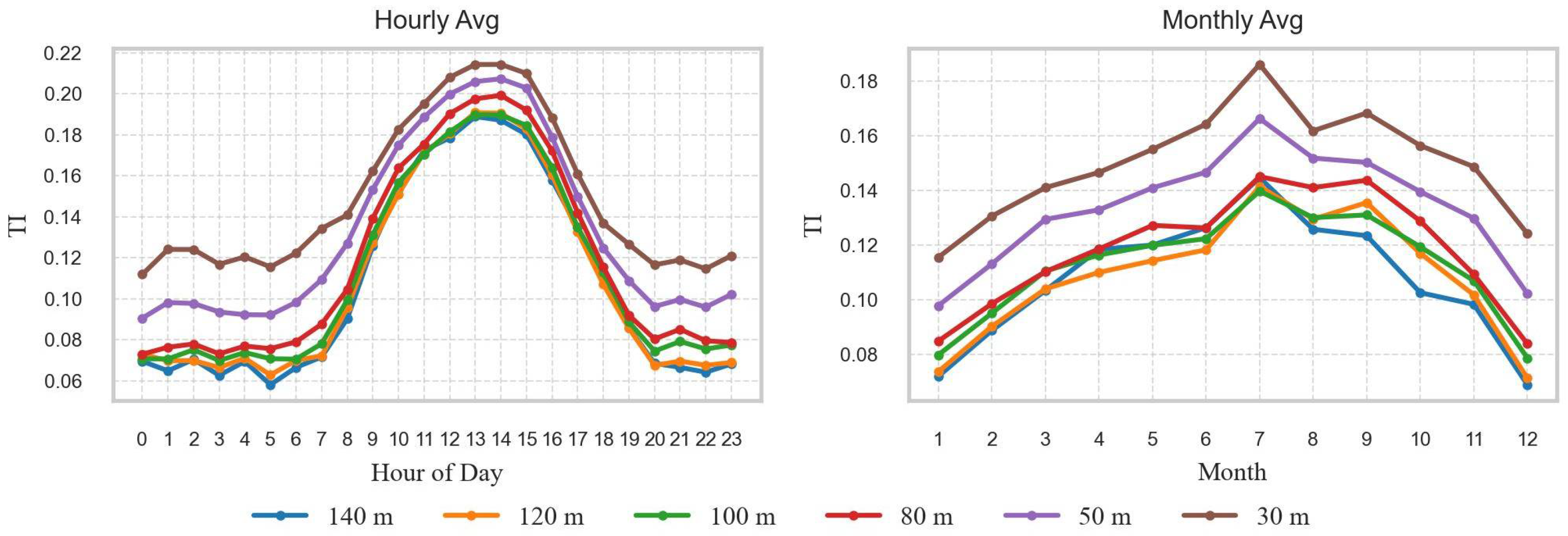
Figure 5 presents the monthly variation in average turbulence intensity (TI) across different heights (left) and the hourly variation in average TI across different heights (right). TI shows a clear seasonal pattern, with lower values during winter months (December–February) and progressively increasing through spring, peaking in summer (June–August), followed by a gradual decline in autumn. Near-surface layers (30 m, 50 m) consistently exhibit higher TI compared to mid-to-upper levels (≥80 m), reflecting stronger surface-induced turbulence effects. The summer peak is particularly pronounced at lower heights, likely due to enhanced convective activity and thermal instability, while the upper layers display relatively moderate seasonal fluctuations, indicating greater atmospheric stability aloft [69]. This vertical and seasonal stratification highlights the influence of surface heating and atmospheric dynamics on turbulence characteristics throughout the year. TI remains relatively low and stable during the nighttime (00:00–06:00), reflecting a stably stratified atmosphere. Following sunrise (07:00–12:00), TI increases progressively, particularly in the near-surface layers (30 m, 50 m), driven by enhanced surface friction and thermally induced turbulence [60,70]. Between noon and late afternoon (12:00–16:00), TI reaches its daily peak, indicating intensified turbulent mixing and strong convective activity. From evening to nighttime (17:00–23:00), surface cooling leads to atmospheric stabilization, and TI gradually decreases, returning to low nighttime levels [69]. Notably, clear vertical stratification is observed: near-ground TI values (30 m, 50 m) are consistently higher than those at mid-to-upper levels (≥80 m), particularly during the day when surface effects are most pronounced, while upper-level TI remains comparatively stable, reflecting reduced sensitivity to surface-induced turbulence [70].

3.3. Performance Evaluation of Wind Power Utilization

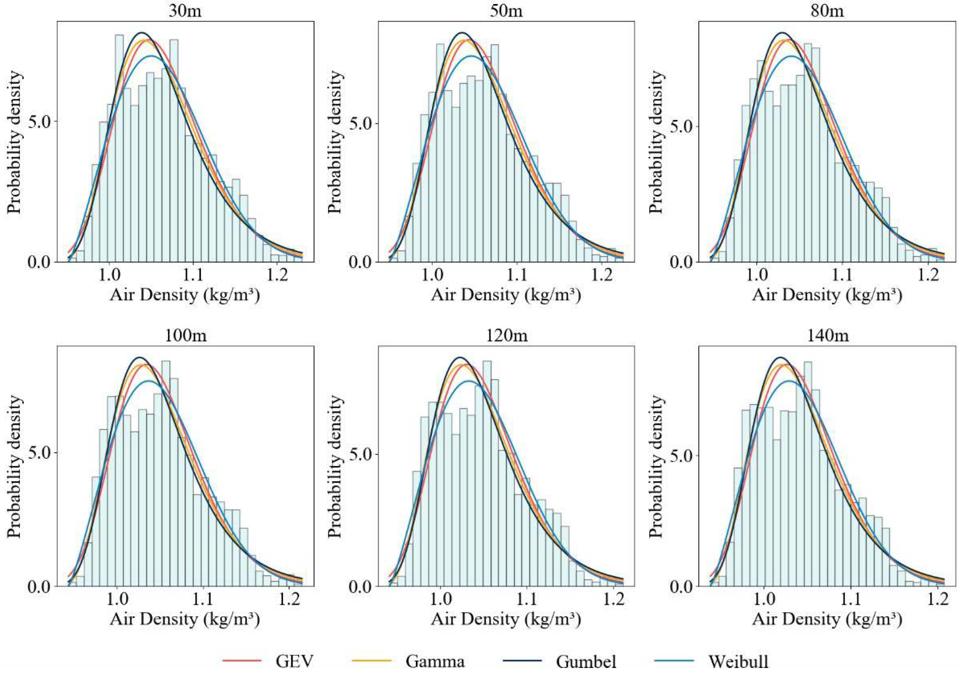
Figure 6 presents the air density probability density distributions across six height levels, along with their fitting performance using various statistical distributions (GEV, Gamma, Gumbel, and Weibull). The results show that the air density distributions at all heights exhibit a pronounced right-skewed pattern, with the distribution peak centered around approximately 1.1 kg/m3. Table 2 presents the K-S statistics evaluating the goodness of fit for various distributions across different heights. The results demonstrate that the Weibull distribution consistently yields the lowest K-S values at all altitude levels, indicating the best fit to the observed wind speed data. Although air density is thermodynamically constrained, its empirically observed probability distribution over long time series can be well characterized by flexible statistical models. Previous work [21] has shown that Weibull-based distributions (e.g., Weibull–Gamma) can accurately fit the empirical distribution of air density and capture its variability for use in joint statistical analyses with wind speed. Consequently, the Weibull distribution was chosen as the baseline model for subsequent wind energy resource assessments.
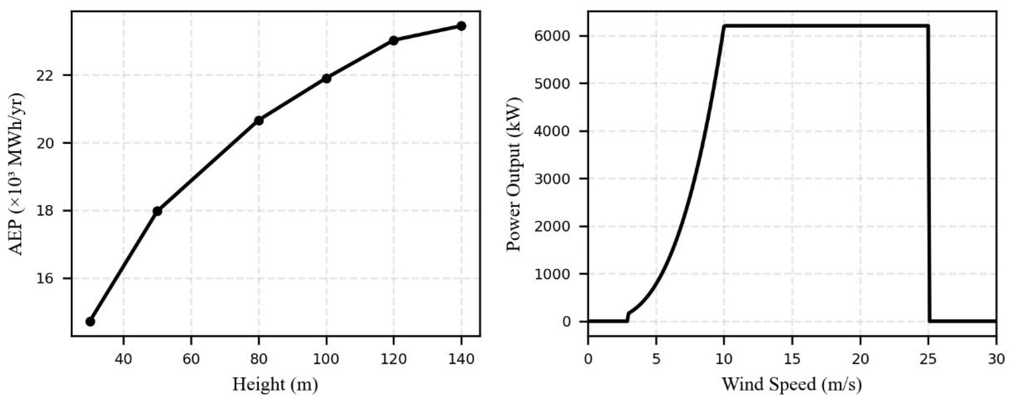
Figure 7 presents the theoretical AEP (left) calculated based on the power curve of the wind turbine used in the study area’s wind farm (right). The results indicate a significant increase in theoretical annual energy production with height, rising from approximately 14.7 × 10³ MWh at 30 m to about 23.5 × 10³ MWh at 140 m, demonstrating that higher altitudes possess richer wind energy resources. This is mainly due to reduced surface friction and increased wind speeds with height, which, given the cubic relationship between wind speed and power, results in significant energy gains [71]. Additionally, higher elevations offer more stable and less turbulent wind conditions, enhancing turbine efficiency and boosting overall annual energy production [19]. Figure 7 (right) shows the turbine power curve, which was used to compute the AEP values and demonstrates the wind speed ranges over which the turbine can operate efficiently.
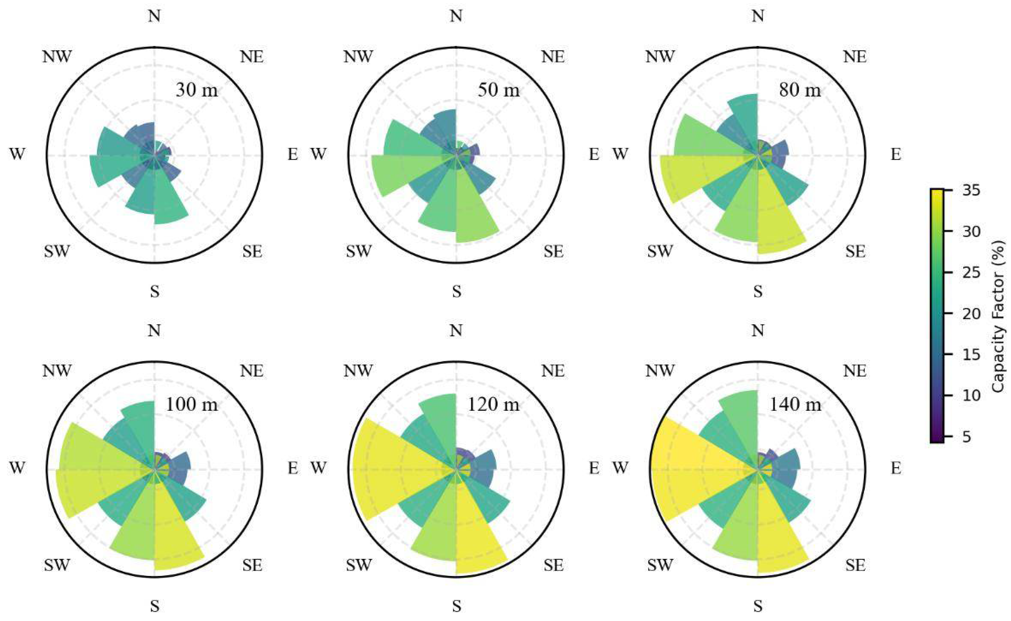
Figure 8 illustrates the capacity factors across different wind directions and heights. Overall, significant differences in capacity factors are observed among various wind directions, with a general increase as height rises. For example, the capacity factors from the southwest and west directions are the highest, exceeding 30%, indicating richer wind resources from these sectors. In contrast, the capacity factors from the east and northeast directions are relatively low, mostly below 15%. This variation is mainly due to the influence of local terrain and climatic conditions on different wind directions, where some directions experience terrain blockage or greater wind speed attenuation, resulting in lower wind energy availability [72,73]. Additionally, as height increases, surface friction decreases and wind speeds increase, leading to higher capacity factors across all directions [59,60]. The elevated capacity factors from the south and southwest winds suggest that these are the dominant wind directions in the region, benefiting from terrain channeling and regional climate systems, thus offering superior wind energy conditions.
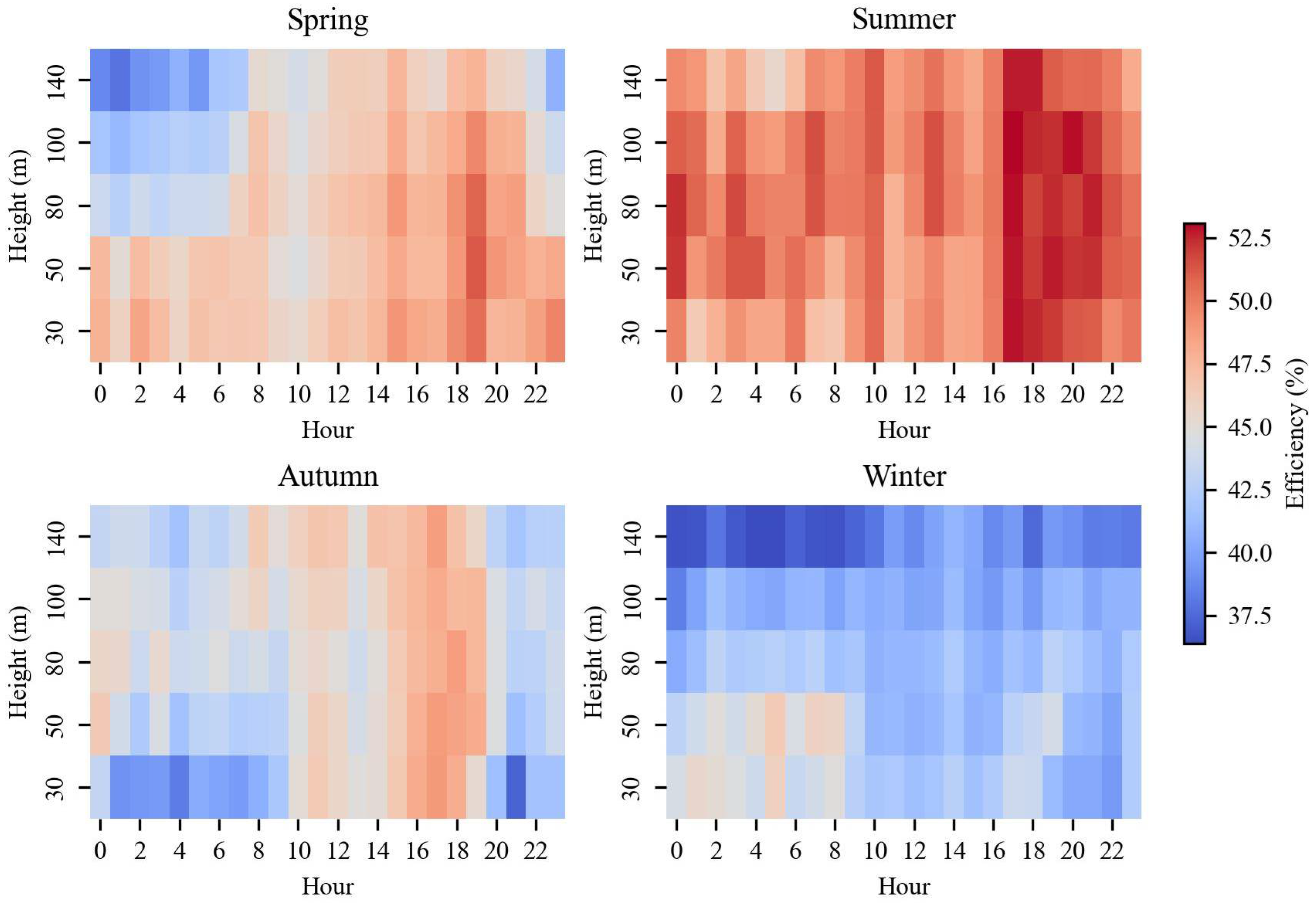
Figure 9 illustrates the variation characteristics of wind turbine power utilization ratio across different heights and time conditions. Overall, the power utilization ratio exhibits a distinct pattern with height, generally improving at higher altitudes due to more stable and stronger wind speeds, which enhance the turbine’s power generation potential. This improvement is mainly because higher altitudes experience less surface friction and turbulence, allowing for more consistent wind flow [60,70]. Seasonal differences are pronounced, with higher efficiency observed in summer, likely attributable to abundant wind resources and stronger winds driven by atmospheric circulation patterns and thermal convection during this period [74,75]. In contrast, although winter generally exhibits higher wind speeds and lower turbulence intensity—conditions that are typically favorable for wind power generation—the power utilization ratio is sometimes lower than in summer. This paradox may be attributed to factors such as more stable but less variable wind directions in winter, which can limit the optimal alignment of turbines and reduce power capture efficiency [30]. Regarding diurnal variation, power utilization ratio peaks from midday to afternoon and drops during nighttime, reflecting the complex interplay of daily solar heating on local atmospheric conditions. During the day, solar radiation heats the surface, causing increased thermal turbulence and mixing in the lower atmosphere [61,62]. Although this raises turbulence intensity and reduces air density, it also decreases wind shear by smoothing vertical wind gradients, which can create more uniform wind profiles favorable for turbine operation. However, near-surface wind speeds may be somewhat lower due to the stabilizing effect of convective mixing on wind speed profiles. At night, the absence of solar heating leads to a more stable atmosphere with reduced turbulence, stronger wind shear, and typically higher wind speeds near turbine hub heights, but the overall power utilization ratio decreases, possibly due to less favorable wind consistency and increased mechanical stresses caused by higher shear [61,62].

3.4. Carbon Emission Reduction Potential

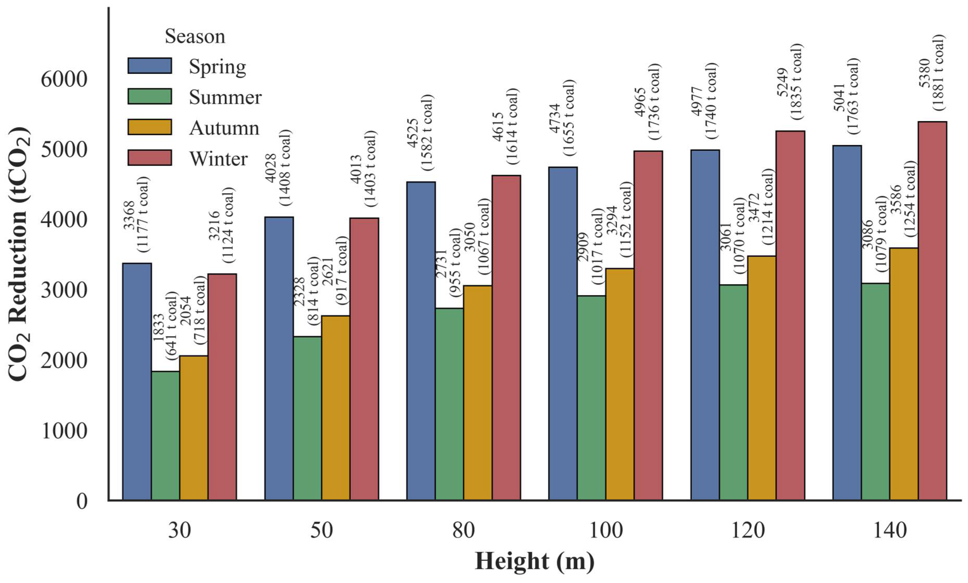
Figure 10 presents the comparison of carbon dioxide (CO2) reduction potential across different hub heights and four seasons in the study area. The results indicate that wind turbines can achieve substantial carbon dioxide mitigation benefits in regions with higher wind speeds (corresponding to increased hub heights), with notable seasonal variations. As the hub height increased from 30 m to 140 m, carbon dioxide reduction in each season exhibited an increasing trend, with the most pronounced reductions observed in spring and winter. Specifically, carbon dioxide reduction in spring increased from 3367.56 t CO2 at a height of 30 m to 5041.13 t CO2 at 140 m, an increase of approximately 49.7%. In winter, reductions were similar, increasing from 3215.72 t CO2 to 5379.99 t CO2, representing an increase of approximately 67.4%. Reductions in autumn and summer were relatively lower, at 3585.72 t CO2 and 3086.37 t CO2 at 140 m, respectively. When converted to standard coal, the emission reduction of a single turbine during high wind speed seasons can reach the equivalent of several thousand tons of standard coal. These results indicate that wind energy power utilization ratio is high in winter and spring, whereas the low wind speeds and increased climatic instability during summer result in relatively limited emission reduction potential. Overall, increasing the hub height of turbines is a critical measure to enhance both power generation and carbon dioxide mitigation, particularly under high wind speed conditions in winter and spring. This is primarily attributable to the high velocity, stability, low turbulence intensity, and concentrated wind energy resources of the winter and spring monsoon in Inner Mongolia [65,75]. Conversely, the weak wind speeds and greater climatic instability in summer reduce wind energy utilization, resulting in comparatively limited carbon mitigation potential.
Using the standard coal carbon emission coefficient (approximately 2.86 t CO2 per ton of standard coal) the 2023 national grid emission factor (EF = 0.0625 t CO2/kWh [76]) for conversion, the results indicate that a carbon dioxide reduction of 5041 t CO2 at a hub height of 140 m in spring corresponds to an approximate saving of 1763 tons of standard coal. In winter, a hub height of 140 m corresponds to approximately 1881 tons of standard coal, while reductions in autumn and summer are approximately 1254 and 1079 tons, respectively. These results suggest that the operation of a single wind turbine across different seasons can not only effectively mitigate regional carbon dioxide emissions, but also achieve energy substitution equivalent to several thousand tons of standard coal. Overall, increasing the hub height of turbines enhances both power generation and carbon dioxide mitigation, particularly under high wind speed conditions in winter and spring, resulting in substantially improved wind energy utilization. This is primarily attributable to the high velocity, stability, low turbulence intensity, and concentrated wind energy resources of the winter and spring monsoon in Inner Mongolia. Conversely, the weak wind speeds and increased climatic instability during summer reduce wind energy utilization, resulting in comparatively limited carbon dioxide mitigation potential.

4. Conclusions

Based on the measured meteorological data from the Hangjinqi wind farm, a systematic analysis was conducted on the near-surface wind field characteristics at different vertical heights within the study area. The investigation focused on key factors affecting wind energy utilization, including vertical wind shear and turbulence, as well as the overall performance of the wind farm and its associated carbon dioxide reduction potential. The study reveals the combined influence of multiple factors on both the development of wind energy resources and their contribution to regional carbon emission mitigation. The main conclusions are summarized as follows:
The annual average wind speed exhibits pronounced seasonal and diurnal variations, with higher wind speeds occurring during winter and spring, particularly in the upper atmospheric layers at night, where speeds can reach up to 10–12 m/s. Conversely, summer and autumn experience relatively weaker winds, especially summer, when wind speeds are influenced by the mixing effects of convective boundary layer currents, resulting in more moderate diurnal fluctuations. The wind speed distribution follows a unimodal right-skewed pattern, predominantly concentrated between 4 and 10 m/s. Notably, as height increases, the frequency peak shifts towards higher wind speed ranges, indicating that elevated altitudes are more favorable for harnessing wind energy.
Analysis of wind shear reveals a significant increase in wind speed aloft during nighttime and in winter and spring, accompanied by elevated wind shear coefficients (α), particularly between the 30–50 m and 100–120 m layers. This pattern reflects the effects of stable atmospheric stratification at night and enhanced downward transport mechanisms, which intensify wind speeds at higher elevations. Turbulence intensity (TI) is elevated during daytime due to thermal surface disturbances but remains comparatively low at night, decreasing with height. These findings suggest that higher-altitude wind energy resources not only exhibit greater abundance but also offer more stable operational conditions, thereby rendering them more suitable for the sustained operation of high-capacity wind turbines.
The estimated annual energy production at the study site ranges from 14.7 × 10³ MWh to 23.5 × 10³ MWh, with capacity factors of 35–42%, exceeding the national average. Wind turbines at higher hub heights (30–140 m) exhibit substantially increased carbon dioxide mitigation across all seasons, with the most pronounced reductions in spring (3367.56–5041.13 t CO2, +49.7%) and winter (3215.72–5379.99 t CO2, +67.4%). When converted to standard coal, a single turbine can save several thousand tons annually, highlighting the potential for significant energy substitution. The high velocity and stability of winter and spring monsoons enhance wind energy utilization, whereas low summer wind speeds limit carbon reduction potential. Overall, raising hub heights is an effective strategy to improve both wind power generation and seasonal carbon mitigation, providing critical support for regional low-carbon energy development.
The wind farm demonstrates excellent wind energy infrastructure, particularly within the 100–140 m altitude range, where the combined effects of consistently high wind speeds and low turbulence intensity throughout the year create an optimal operating environment for large-scale wind turbines. Therefore, it is recommended that future installations prioritize turbines with tower heights of 140 m or greater to fully capitalize on the stronger and more stable wind resources at elevated levels. Through comprehensive analysis of wind shear and turbulence distribution across the site, turbine spacing and layout can be optimized to minimize wake losses and maximize overall power output. Additionally, the implementation of intelligent scheduling and power forecasting systems—incorporating seasonal and diurnal wind field variations—can enable more precise load management and prediction, thereby enhancing equipment utilization and grid integration efficiency.

Author Contributions

Conceptualization, L.J. (Li Jiang); methodology, L.J. (Li Jiang); software, L.J. (Li Jiang); validation, C.S.; formal analysis, L.J. (Li Jiang); investigation, L.J. (Li Jiang); resources, S.Z., L.C., X.M. and L.J. (Ligang Jiang); data curation, L.J. (Li Jiang); writing—original draft preparation, L.J. (Li Jiang); writing—review and editing, C.S., T.Z.; visualization, L.J. (Li Jiang); supervision, C.S.; project administration, X.J.; funding acquisition, C.S. All authors have read and agreed to the published version of the manuscript.

Funding

The research was funded by the National Natural Science Foundation of China (31570708) and the National Key Scientific and Technological Infrastructure project “Earth System Science Numerical Simulator Facilit” (Earth Lab).

Data Availability Statement

The data and material analyzed in this current study are available from the corresponding author on reasonable request.

Conflicts of Interest

Authors Shijia Zhang, Lvbing Cao were employed by the Powerchina Beijing Engineering Corporation Limited. Authors Xiangdong Meng, Liigang Jiang were employed by the Huaneng Renewables Corporation Limited Mengxi Branch. The remaining authors declare that the research was conducted in the absence of any commercial or financial relationships that could be construed as a potential conflict of interest.

References

  1. Thomas, B.; Costoya, X.; DeCastro, M.; Insua-Costa, D.; Senande-Rivera, M.; Gómez-Gesteira, M. Downscaling CMIP6 climate projections to classify the future offshore wind energy resource in the Spanish territorial waters. J. Clean. Prod. 2023, 433, 139860. [Google Scholar] [CrossRef]
  2. Chen, Y.; Zhang, D.; Qi, W.; Guo, P.; Li, J. Power prediction of a Savonius wind turbine cluster considering wind direction characteristics on three sites. J. Clean. Prod. 2023, 423, 138789. [Google Scholar] [CrossRef]
  3. Ma, K.; Zhang, H.; Gao, X.; Wang, X.; Nian, H.; Fan, W. Research on Evaluation Method of Wind Farm Wake Energy Efficiency Loss Based on SCADA Data Analysis. Sustainability 2024, 16, 1813. [Google Scholar] [CrossRef]
  4. Murthy, K.S.R.; Rahi, O.P. A comprehensive review of wind resource assessment. Renew. Sustain. Energy Rev. 2017, 72, 1320–1342. [Google Scholar] [CrossRef]
  5. Ouerghi, F.H.; Omri, M.; Menaem, A.A.; Taloba, A.I.; Abd El-Aziz, R.M. Feasibility evaluation of wind energy as a sustainable energy resource. Alex. Eng. J. 2024, 106, 227–239. [Google Scholar] [CrossRef]
  6. Wang, C. China Hit New Record of Solar and Wind Power Capacity Additions in 2024; Climate Energy Finance location: Sydney, Australia, 2025. [Google Scholar]
  7. Xue, B.; Ma, Z.; Geng, Y.; Heck, P.; Ren, W.; Tobias, M.; Maas, A.; Jiang, P.; Puppim De Oliveira, J.A.; Fujita, T. A life cycle co-benefits assessment of wind power in China. Renew. Sustain. Energy Rev. 2015, 41, 338–346. [Google Scholar] [CrossRef]
  8. Jung, C.; Schindler, D. Global trends of wind direction-dependent wind resource. Energy 2024, 304, 132235. [Google Scholar] [CrossRef]
  9. Pelser, T.; Weinand, J.M.; Kuckertz, P.; McKenna, R.; Linssen, J.; Stolten, D. Reviewing accuracy & reproducibility of large-scale wind resource assessments. Adv. Appl. Energy 2024, 13, 100158. [Google Scholar]
  10. Sari, F.; Yalcin, M. Investigation of the importance of criteria in potential wind farm sites via machine learning algorithms. J. Clean. Prod. 2024, 435, 140575. [Google Scholar] [CrossRef]
  11. Oliveira, T.; Varum, C.; Botelho, A. Wind power and CO2 emissions in the Irish market. Energy Econ. 2019, 80, 48–58. [Google Scholar] [CrossRef]
  12. Yang, F.; Sun, L.; Wang, J. Monthly variation and correlation analysis of global temperature and wind resources under climate change. Energy Convers. Manag. 2023, 285, 116992. [Google Scholar] [CrossRef]
  13. Lu, Y.; Wu, B.; Yan, N.; Zhu, W.; Zeng, H.; Ma, Z.; Xu, J.; Wu, X.; Pang, B. Quantifying the Contributions of Environmental Factors to Wind Characteristics over 2000–2019 in China. ISPRS Int. J. Geo-Inf. 2021, 10, 515. [Google Scholar] [CrossRef]
  14. Wang, Y.; Shen, R.; Ma, M. Research on ultra-short term forecasting technology of wind power output based on various meteorological factors. Energy Rep. 2022, 8, 1145–1158. [Google Scholar] [CrossRef]
  15. Elshafei, B.; Popov, A.; Giddings, D. Enhanced offshore wind resource assessment using hybrid data fusion and numerical models. Energy 2024, 310, 133208. [Google Scholar] [CrossRef]
  16. Zhu, Y.; Zhong, S.; Shen, L.; Li, D.; Zhao, J.; Hou, X. From potential to utilization: Exploring the optimal layout with the technical path of wind resource development in Tibet. Energy Convers. Manag. 2024, 304, 118231. [Google Scholar] [CrossRef]
  17. Arrieta-Prieto, M.E.; Schell, K.R. Data-driven optimization for wind farm siting. Int. J. Electr. Power 2024, 155, 109552. [Google Scholar] [CrossRef]
  18. Dayal, K.K.; Cater, J.E.; Kingan, M.J.; Bellon, G.D.; Sharma, R.N. Wind resource assessment and energy potential of selected locations in Fiji. Renew. Energy 2021, 172, 219–237. [Google Scholar] [CrossRef]
  19. Liu, J.; Gao, C.Y.; Ren, J.; Gao, Z.; Liang, H.; Wang, L. Wind resource potential assessment using a long term tower measurement approach: A case study of Beijing in China. J. Clean. Prod. 2018, 174, 917–926. [Google Scholar] [CrossRef]
  20. Floors, R.; Nielsen, M. Estimating Air Density Using Observations and Re-Analysis Outputs for Wind Energy Purposes. Energies 2019, 12, 2038. [Google Scholar] [CrossRef]
  21. Liang, Y.; Wu, C.; Ji, X.; Zhang, M.; Li, Y.; He, J.; Qin, Z. Estimation of the influences of spatiotemporal variations in air density on wind energy assessment in China based on deep neural network. Energy 2022, 239, 122210. [Google Scholar] [CrossRef]
  22. Ulazia, A.; Sáenz, J.; Ibarra-Berastegi, G.; González-Rojí, S.J.; Carreno-Madinabeitia, S. Global estimations of wind energy potential considering seasonal air density changes. Energy 2019, 187, 115938. [Google Scholar] [CrossRef]
  23. Jung, C.; Schindler, D. Introducing a new approach for wind energy potential assessment under climate change at the wind turbine scale. Energy Convers. Manag. 2020, 225, 113425. [Google Scholar] [CrossRef]
  24. Kim, D.; Kim, Y.; Kim, B. Changes in wind turbine power characteristics and annual energy production due to atmospheric stability, turbulence intensity, and wind shear. Energy 2021, 214, 119051. [Google Scholar] [CrossRef]
  25. Juan, Y.H.; Wen, C.Y.; Chen, W.Y.; Yang, A.S. Numerical assessments of wind power potential and installation arrangements in realistic highly urbanized areas. Renew. Sustain. Energy Rev. 2021, 135, 110165. [Google Scholar] [CrossRef]
  26. Jung, C.; Schindler, D.; Laible, J.; Buchholz, A. Introducing a system of wind speed distributions for modeling properties of wind speed regimes around the world. Energy Convers. Manag. 2017, 144, 181–192. [Google Scholar] [CrossRef]
  27. Dai, J.; Tan, Y.; Yang, W.; Wen, L.; Shen, X. Investigation of wind resource characteristics in mountain wind farm using multiple-unit SCADA data in Chenzhou: A case study. Energy Convers. Manag. 2017, 148, 378–393. [Google Scholar] [CrossRef]
  28. Qin, Z.; Li, W.; Xiong, X. Generation System Reliability Evaluation Incorporating Correlations of Wind Speeds With Different Distributions. IEEE Trans. Power Syst. 2013, 28, 551–558. [Google Scholar] [CrossRef]
  29. Hou, A.; Ni, G.; Yang, H.; Lei, Z. Numerical Analysis on the Contribution of Urbanization to Wind Stilling: An Example over the Greater Beijing Metropolitan Area. J. Appl. Meteorol. Clim. 2013, 52, 1105–1115. [Google Scholar] [CrossRef]
  30. Jiang, L.; Ji, X.D.; Yang, S.H.; Zhang, Z.Y. Assessment of wind resource potential at different heights in urban areas: A case study of Beijing. Renew. Energy 2025, 248, 123175. [Google Scholar] [CrossRef]
  31. He, J.Y.; Chan, P.W.; Li, Q.S.; Huang, T.; Yim, S.H.L. Assessment of urban wind energy resource in Hong Kong based on multi-instrument observations. Renew. Sustain. Energy Rev. 2024, 191, 114123. [Google Scholar] [CrossRef]
  32. Vallejo Díaz, A.; Herrera Moya, I.; Castellanos, J.E.; Garabitos Lara, E. Optimal Positioning of Small Wind Turbines Into a Building Using On-Site Measurements and Computational Fluid Dynamic Simulation. J. Energy Resour. Technol. 2024, 146, 081801. [Google Scholar] [CrossRef]
  33. Jung, C.; Sander, L.; Schindler, D. Future global offshore wind energy under climate change and advanced wind turbine technology. Energy Convers. Manag. 2024, 321, 119075. [Google Scholar] [CrossRef]
  34. Chen, X.; Wang, Y.; Wu, Z.; Zhou, M.; Yuan, B. Capacity expansion model for multi-temporal energy storage in renewable energy base considering various transmission utilization rates. J. Energy Storage 2024, 98, 113145. [Google Scholar] [CrossRef]
  35. Shi, R.; Fan, X.; He, Y. Comprehensive evaluation index system for wind power utilization levels in wind farms in China. Renew. Sustain. Energy Rev. 2017, 69, 461–471. [Google Scholar] [CrossRef]
  36. Capelletti, M.; Raimondo, D.M.; De Nicolao, G. Wind power curve modeling: A probabilistic Beta regression approach. Renew. Energy 2024, 223, 119970. [Google Scholar] [CrossRef]
  37. Qiao, Y.; Han, S.; Zhang, Y.; Liu, Y.; Yan, J. A multivariable wind turbine power curve modeling method considering segment control differences and short-time self-dependence. Renew. Energy 2024, 222, 119894. [Google Scholar] [CrossRef]
  38. Wu, H.; Chen, Y.; Cai, Z.; Heidari, A.A.; Chen, H.; Liang, G. Dual-weight decay mechanism and Nelder-Mead simplex boosted RIME algorithm for optimal power flow. J. Big Data 2024, 11, 172. [Google Scholar] [CrossRef]
  39. Cai, W.; Hu, Y.; Fang, F.; Yao, L.; Liu, J. Wind farm power production and fatigue load optimization based on dynamic partitioning and wake redirection of wind turbines. Appl. Energy 2023, 339, 121000. [Google Scholar] [CrossRef]
  40. Liu, Y.; Zhao, Z.; Liu, Y.; Liu, H.; Wei, S.; Ma, Y.; Ling, Z.; Luo, Q. Combined wake control of aligned wind turbines for power optimization based on a 3D wake model considering secondary wake steering. Energy 2024, 308, 132900. [Google Scholar] [CrossRef]
  41. Peng, H.; Li, S.; Shangguan, L.; Fan, Y.; Zhang, H. Analysis of Wind Turbine Equipment Failure and Intelligent Operation and Maintenance Research. Sustainability 2023, 15, 8333. [Google Scholar] [CrossRef]
  42. Howland, M.F.; Quesada, J.B.; Martínez, J.J.P.; Larrañaga, F.P.; Yadav, N.; Chawla, J.S.; Sivaram, V.; Dabiri, J.O. Collective wind farm operation based on a predictive model increases utility-scale energy production. Nat. Energy 2022, 7, 818–827. [Google Scholar] [CrossRef]
  43. Yao, J.; Pei, J.; Xu, D.; Liu, R.; Wang, X.; Wang, C.; Li, Y. Coordinated control of a hybrid wind farm with DFIG-based and PMSG-based wind power generation systems under asymmetrical grid faults. Renew. Energy 2018, 127, 613–629. [Google Scholar] [CrossRef]
  44. Dhiman, H.S.; Deb, D. Wake management based life enhancement of battery energy storage system for hybrid wind farms. Renew. Sustain. Energy Rev. 2020, 130, 109912. [Google Scholar] [CrossRef]
  45. Zhang, B.; Xu, G.; Zhang, Z. A holistic robust method for optimizing multi-timescale operations of a wind farm with energy storages. J. Clean. Prod. 2022, 356, 131793. [Google Scholar] [CrossRef]
  46. Yi, D.; Choi, H.; Lee, S.; Lee, Y.H. Understanding the Characteristics of Vertical Structures for Wind Speed Observations via Wind-LIDAR on Jeju Island. Atmosphere 2023, 14, 1260. [Google Scholar] [CrossRef]
  47. Orlov, A.; Sillmann, J.; Vigo, I. Better seasonal forecasts for the renewable energy industry. Nat. Energy 2020, 5, 108–110. [Google Scholar] [CrossRef]
  48. Wang, J.; Qin, S.; Jin, S.; Wu, J. Estimation methods review and analysis of offshore extreme wind speeds and wind energy resources. Renew. Sustain. Energy Rev. 2015, 42, 26–42. [Google Scholar] [CrossRef]
  49. Yang, S.; Ji, X.; Tao, Y.; Jia, J.; Zhang, Z.; Jiang, L. Study on Non-Stationary Wind Speed Models and Wind Load Design Parameters Based on Data from the Beijing 325 m Meteorological Tower, 1991–2020. Appl. Sci. 2024, 14, 3979. [Google Scholar] [CrossRef]
  50. Zhang, L.; Zhang, Z.; Wu, C.; Ji, X.; Xue, X.; Jiang, L.; Yang, S. Joint Probability Distribution of Extreme Wind Speed and Air Density Based on the Copula Function to Evaluate Basic Wind Pressure. Atmosphere 2024, 15, 1437. [Google Scholar] [CrossRef]
  51. Anghel, C.G. Revisiting the Use of the Gumbel Distribution: A Comprehensive Statistical Analysis Regarding Modeling Extremes and Rare Events. Mathematics 2024, 12, 2466. [Google Scholar] [CrossRef]
  52. Chang, T.P. Estimation of wind energy potential using different probability density functions. Appl. Energy 2011, 88, 1848–1856. [Google Scholar] [CrossRef]
  53. Jung, C.; Schindler, D. The role of air density in wind energy assessment—A case study from Germany. Energy 2019, 171, 385–392. [Google Scholar] [CrossRef]
  54. Zhang, Z.; Liang, Y.; Xue, X.; Li, Y.; Zhang, M.; Li, Y.; Ji, X. China’s future wind energy considering air density during climate change. Renew. Sust. Energy Rev. 2024, 199, 114452. [Google Scholar] [CrossRef]
  55. Hur, J. Potential capacity factor estimates of wind generating resources for transmission planning. Renew. Energy 2021, 179, 1742–1750. [Google Scholar] [CrossRef]
  56. Yao, Y.; Xu, J.; Sun, D. Untangling global levelised cost of electricity based on multi-factor learning curve for renewable energy: Wind, solar, geothermal, hydropower and bioenergy. J. Clean. Prod. 2021, 285, 124827. [Google Scholar] [CrossRef]
  57. Tong, D.; Farnham, D.J.; Duan, L.; Zhang, Q.; Lewis, N.S.; Caldeira, K.; Davis, S.J. Geophysical constraints on the reliability of solar and wind power worldwide. Nat. Commun. 2021, 12, 6146. [Google Scholar] [CrossRef]
  58. Gao, W.; Han, M.; Chen, L.; Ai, C.; Liu, S.; Cao, S.; Wei, L. Life cycle carbon emission accounting of a typical coastal wind power generation project in Hebei Province, China. Energy Convers. Manag. 2025, 324, 119243. [Google Scholar] [CrossRef]
  59. Li, B.; Han, Z.; Zhang, X.; Yang, Q.; Li, C.; Sun, L. Investigation of the vertically-layered structure and surface roughness parameters of the urban boundary layer. Struct. Des. Tall Spec. Build. 2023, 32, e2056. [Google Scholar] [CrossRef]
  60. Zhang, Z.; Wang, K.; Chen, D.; Li, J.; Dickinson, R. Increase in Surface Friction Dominates the Observed Surface Wind Speed Decline during 1973–2014 in the Northern Hemisphere Lands. J. Clim. 2019, 32, 7421–7435. [Google Scholar] [CrossRef]
  61. Lampert, A.; Bernalte Jimenez, B.; Gross, G.; Wulff, D.; Kenull, T. One-year observations of the wind distribution and low-level jet occurrence at Braunschweig, North German Plain. Wind Energy 2016, 19, 1807–1817. [Google Scholar] [CrossRef]
  62. Zhou, C.; Mamtimin, A.; Yang, F.; Huo, W.; Wang, M.; Pan, H.; He, Q.; Jin, L.; Yang, X. Dust uplift potential in the Taklimakan Desert: An analysis based on different wind speed measurement intervals. Theor. Appl. Climatol. 2019, 137, 1449–1456. [Google Scholar] [CrossRef]
  63. Huang, X.; Zhu, J.; Li, Y. Temperature analysis of steel box girder considering actual wind field. Eng. Struct. 2021, 246, 113020. [Google Scholar] [CrossRef]
  64. Zeng, X.; Wang, M.; Wang, N.; Yi, X.; Chen, C.; Zhou, Z.; Wang, G.; Zheng, Y. Assessing simulated summer 10-m wind speed over China: Influencing processes and sensitivities to land surface schemes. Clim. Dynam. 2018, 50, 4189–4209. [Google Scholar] [CrossRef]
  65. Chang, T.; Ko, H.; Liu, F.; Chen, P.; Chang, Y.; Liang, Y.; Jang, H.; Lin, T.; Chen, Y. Fractal dimension of wind speed time series. Appl. Energy 2012, 93, 742–749. [Google Scholar] [CrossRef]
  66. Li, J.; Wang, X.; Yu, X.B. Use of spatio-temporal calibrated wind shear model to improve accuracy of wind resource assessment. Appl. Energy 2018, 213, 469–485. [Google Scholar] [CrossRef]
  67. Mahrt, L.; Richardson, S.; Stauffer, D.; Seaman, N. Nocturnal wind-directional shear in complex terrain. Q. J. R. Meteorol. Soc. 2014, 140, 2393–2400. [Google Scholar] [CrossRef]
  68. Guan, X.; Huang, J.; Guo, R.; Yu, H.; Lin, P.; Zhang, Y. Role of radiatively forced temperature changes in enhanced semi-arid warming in the cold season over east Asia. Atmos. Chem. Phys. 2015, 15, 13777–13786. [Google Scholar] [CrossRef]
  69. Du, B.; Ge, M.; Zeng, C.; Cui, G.; Liu, Y. Influence of atmospheric stability on wind-turbine wakes with a certain hub-height turbulence intensity. Phys. Fluids 2021, 33, 055111. [Google Scholar] [CrossRef]
  70. Ren, G.; Liu, J.; Wan, J.; Li, F.; Guo, Y.; Yu, D. The analysis of turbulence intensity based on wind speed data in onshore wind farms. Renew. Energy 2018, 123, 756–766. [Google Scholar] [CrossRef]
  71. Kim, D.; Kim, B. Differences in wind farm energy production based on the atmospheric stability dissipation rate: Case study of a 30 MW onshore wind farm. Energy 2022, 239, 122380. [Google Scholar] [CrossRef]
  72. Chen, F.; Wang, W.; Gu, Z.; Zhu, Y.; Li, Y.; Shu, Z. Investigation of hilly terrain wind characteristics considering the interference effect. J. Wind. Eng. Ind. Aerod. 2023, 241, 105543. [Google Scholar] [CrossRef]
  73. Sun, H.; Yang, H.; Gao, X. Investigation into wind turbine wake effect on complex terrain. Energy 2023, 269, 126767. [Google Scholar] [CrossRef]
  74. de Szoeke, S.P.; Bretherton, C.S. Variability in the Southerly Flow into the Eastern Pacific ITCZ. J. Atmos. Sci. 2005, 62, 4400–4411. [Google Scholar] [CrossRef]
  75. Wang, B.; Ho, L. Rainy Season of the Asian–Pacific Summer Monsoon. J. Clim. 2005, 15, 386–398. [Google Scholar] [CrossRef]
  76. Ministry of Ecology and Environment; National Bureau of Statistics. Announcement on the Release of 2023 Power Carbon Dioxide Emission Factors; Ministry of Ecology and Environment and National Bureau of Statistics: Beijing, China, 2025. Available online: https://www.mee.gov.cn/xxgk2018/xxgk/xxgk01/202512/t20251231_1139517.html (accessed on 15 January 2026).
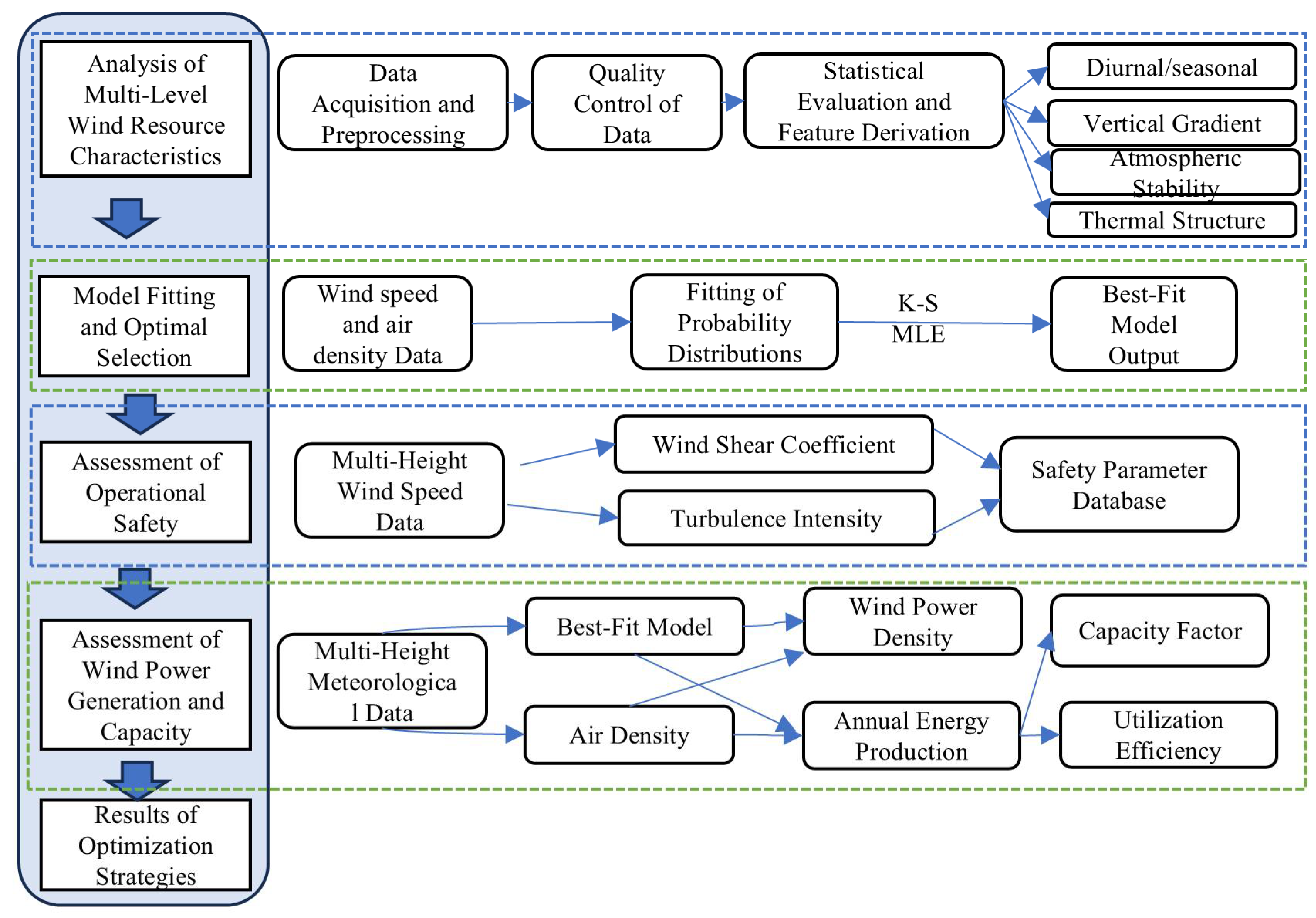
Figure 1. Workflow of the wind resource assessment and modeling framework.
Atmosphere 17 00102 g001
Figure 2. Seasonal and Diurnal Heatmap of Wind Speeds at Different Heights.
Atmosphere 17 00102 g002
Figure 3. Probability Histograms of Wind Speed with Fitted fitting results.
Atmosphere 17 00102 g003
Figure 4. Monthly and Diurnal Pattern of Wind Shear.
Atmosphere 17 00102 g004
Figure 5. Monthly and Diurnal Pattern of Turbulence Intensity.
Atmosphere 17 00102 g005
Figure 6. Probability Histograms of Air Density at Different Heights with Fitted fitting results.
Atmosphere 17 00102 g006
Figure 7. Theoretical Annual Energy Production and Power Curve of the Generator.
Atmosphere 17 00102 g007
Figure 8. Capacity Factor at Different Directions and Heights.
Atmosphere 17 00102 g008
Figure 9. Heatmap of Wind Turbine Utilization Efficiency by Hour and Height.
Atmosphere 17 00102 g009
Figure 10. Seasonal variation of CO2 reduction potential at different heights.
Atmosphere 17 00102 g010
Table 1. Statistical Values of K-S for Different Fitting Functions of Wind Speed.
HeightGEVGammaGumbelWeibull
30 m0.01310.01490.03130.0099
50 m0.01230.01240.02750.0067
80 m0.01530.01460.02820.0074
100 m0.01410.01360.02740.0092
120 m0.01450.01250.02770.0097
140 m0.01570.01200.02450.0108
Table 2. Statistical Values of K-S for Different Fitting Functions of Air Density.
HeightGEVGammaGumbelWeibull
30 m0.04280.03380.04400.0333
50 m0.04300.03440.04410.0337
80 m0.04210.03580.04510.0329
100 m0.04100.03720.04600.0320
120 m0.04010.03650.04500.0305
140 m0.03920.03740.04540.0299
Disclaimer/Publisher’s Note: The statements, opinions and data contained in all publications are solely those of the individual author(s) and contributor(s) and not of MDPI and/or the editor(s). MDPI and/or the editor(s) disclaim responsibility for any injury to people or property resulting from any ideas, methods, instructions or products referred to in the content.