Synoptic Ocean–Atmosphere Coupling at the Intertropical Convergence Zone and Its Vicinity in the Western Tropical Atlantic Ocean

Abstract

In the Atlantic Ocean, the Intertropical Convergence Zone (ITCZ) sustains the climate of northeastern Brazil and northwestern Africa by modulating their rainy and dry seasons. Using observational data, radiosondes and Expendable Bathythermographs (XBTs), we investigated short-term ocean–atmosphere coupling across the ITCZ region along the 38° W meridian. The data represents synchronous measurements of the marine atmospheric boundary layer (MABL) and the ocean’s mixed layer (OML) for the period between 17 October and 8 November 2018. The ITCZ demonstrated pronounced variability in position, intensity, and width, driven by the changes in the predominance of northeast and southeast trade winds. These atmospheric changes directly impacted the Equatorial Divergence (ED), which transitioned from an asymmetric structure with shallower isothermal layer depths (ILDs) (~−14 m) around 11° N to a more homogenous region between 5° N and 10° N, with an average ILD of −21.83 ± 5.23 m. A comparison with ORAS5 and WOA23 indicates that the products reproduce the vertical thermal structure of the WTAO well (r² > 0.9) but systematically overestimate the temperature at the bottom of the ILD by 3–4 °C. The difference between the ILD and the mixed layer depth (MLD) is more pronounced south of the ED due to the Amazon River salinity front, advected by the NECC, but the ILD estimated from XBT data closely matches the MLD estimated for ORAS5 and WOA23 in the ED region. These unprecedented observations showcase, for the first time, short-term ocean–atmosphere coupled variability across the WTAO ITCZ region, highlighting the importance of atmospheric synoptic-scale processes in modulating the OML and the ED.

1. Introduction

Understanding ocean–atmosphere interactions on multiple space and time scales within the Atlantic Ocean basin is essential to comprehending the climate variability of the South American and African continents [1,2,3,4]. In the Tropical Atlantic Ocean (TAO), the Intertropical Convergence Zone (ITCZ) is one of the main meteorological systems, characterized by its pronounced seasonal variability [5,6]. When the ITCZ shifts northward (southward) in austral winter–spring (summer–fall), it is accompanied by the sea surface temperature (SST) maximum band, the equatorial atmospheric pressure trough, the trade winds convergence zone (TWCZ), and the observed precipitation maxima of northeastern South America and northwestern Africa [7,8,9]. By studying and characterizing these features and phenomena, which might not coincide spatially at all times, the dynamics of the ITCZ have already been well described.

Using both observational and modeling data, Cabos et al. [3] reported that the seasonal meridional migration of the ITCZ is one of the main drivers of TAO variability. The authors also state that several systematic errors still cause persistent biases in global, ocean–atmosphere coupled models, leading to a misrepresentation of the ITCZ position. This can directly impact climate predictability in the tropics, especially along the coasts of northeastern Brazil and western Africa. These biases, attributed to misrepresented physics and poor resolutions of some atmospheric and oceanic features, are common in both the Pacific and Atlantic ITCZs and have been studied and continue to be explored by many, such as Doi et al. [10]; Richter et al. [11]; Siongco et al. [12]; Laurido et al. [13]; Lee et al. [14]; Luo et al. [15], and Dong et al. [16].

Although the climate characteristics of the ITCZ from synoptic to decadal scales are relatively well known [17,18,19,20], the characterization of the ITCZ at the synoptic meteorological scale and its direct impacts on the underlying waters still lack further investigation. Wang and Magnusdottir [19], for instance, used remote sensing data to investigate the cloud band breakdown of the ITCZ in the central and eastern Pacific. Nogueira et al. [21] used a precipitation-based algorithm to identify the mean ITCZ position for short time scales and to describe its climatology for the TAO. Diedhiou et al. [17] described how the Atlantic ITCZ is influenced by westward-propagating waves, which consequently impact rainfall in West Africa over a 3 to 9-day period. This time scale was also observed by Serra and Houze Jr. [18] when studying the temporal variability of the meridional component of wind and humidity. The authors are among the few who used radiosonde profiles in the eastern Pacific to study the ITCZ. Goswami et al. [22], on the other hand, reported a 10 to 20-day variability in the ITCZ position using a zonally symmetric climate model. Still examining shorter time scales when studying the ITCZ, Wang and Fu [20] used satellite estimates of outgoing longwave radiation (OLR) and precipitation rates to investigate how convection-induced, eastward-propagating atmospheric waves from the Amazon rainforest modulate atmospheric convection in the Atlantic ITCZ.

Although not conceived to specifically monitor the ITCZ, the PIRATA (Prediction and Research Moored Array in the Tropical Atlantic) Program has maintained an array of 18 moored buoys in the TAO since the 1990s. The buoys are equipped with meteorological and oceanographic sensors [9,23,24] that provide long-term, in situ measurements of ocean–atmosphere properties and can be used, among other things, to validate or be assimilated into models. The program is conducted by Brazil, France, and the United States. Although conceived to provide data for ocean–atmosphere studies, especially those related to seasonal forecasts, most results from the PIRATA array were primarily related to oceanography. Foltz et al. [1,25,26], for instance, used PIRATA data to study the mixed layer heat content and salt budgets in the TAO. These authors, however, report that these properties presented a seasonal variability closely related to the ITCZ. When investigating the ocean’s mixed layer (OML) below the ITCZ, the Ekman drive causes a shallow mixed layer known as the Equatorial Divergence (ED) [1,26,27], which is strongest in austral spring [28].

Faria et al. [29] have also investigated the influence of the ITCZ at shorter temporal scales in the western TAO (WTAO) region, describing the role of atmospheric convergence in modulating the westward transport of Saharan aerosols into the western portion of the Tropical Atlantic. The authors describe for the first time that trace metals such as iron and aluminum are concentrated at the sea surface just below the ITCZ by the deposition of aerosols transported toward the WTAO. Musetti de Assis et al. [30], using 20 years of PIRATA data, studied the carbonate system in the WTAO. The authors emphasized the importance of the ITCZ position, as well as the Amazon River discharge, for modulating the variability of salinity in the study region. Due to the simultaneous effects of aerosol deposition and the Amazon River’s output, the WTAO region is one of the critical regions in the global ocean for primary production, photosynthesis, respiration, and carbon cycling in open waters [29,30,31,32,33,34].

The WTAO is also an important agent in oceanic meridional heat transport through the warm branch of the Atlantic Meridional Overturning Circulation (AMOC). This branch is represented in the region by the North Brazil Undercurrent (NBUC), the North Brazil Current (NBC), and the eddies that form at the NBC retroflection [35,36,37]. Considering that conclusive studies about the coupling mechanisms between the ocean and the atmosphere in the WTAO, especially under the ITCZ and its vicinity, are still lacking, this work aims to describe the spatial and temporal variability of atmospheric variables within the MABL and the consequent impacts on the OML along the 38° W meridian within a period of 21 days. We used data collected from 17 October to 8 November 2018, taken in situ between 5° S and 15° N using radiosondes and Expendable Bathythermographs (XBTs), as well as both oceanic reanalysis and climatology atlas data to provide a description of ocean–atmosphere coupling and its variability between two consecutive routes along the same transect. We also investigated the mean signature of water temperature in the OML observed in situ during the period of this study and assessed the biases with respect to other databases.

This paper is divided into the following sections: In Session 2, we present our material and methods, including the study area and period, as well as the instruments, data, and methods used for sampling the transects used in this work. We also present the statistical methods used to compare different datasets; Session 3 presents the results and discussion: here we divide the results and discussion on both atmosphere and ocean, making a link between the two systems and discussing the results. Session 4 presents our conclusions.

2. Materials and Methods

2.1. Study Area

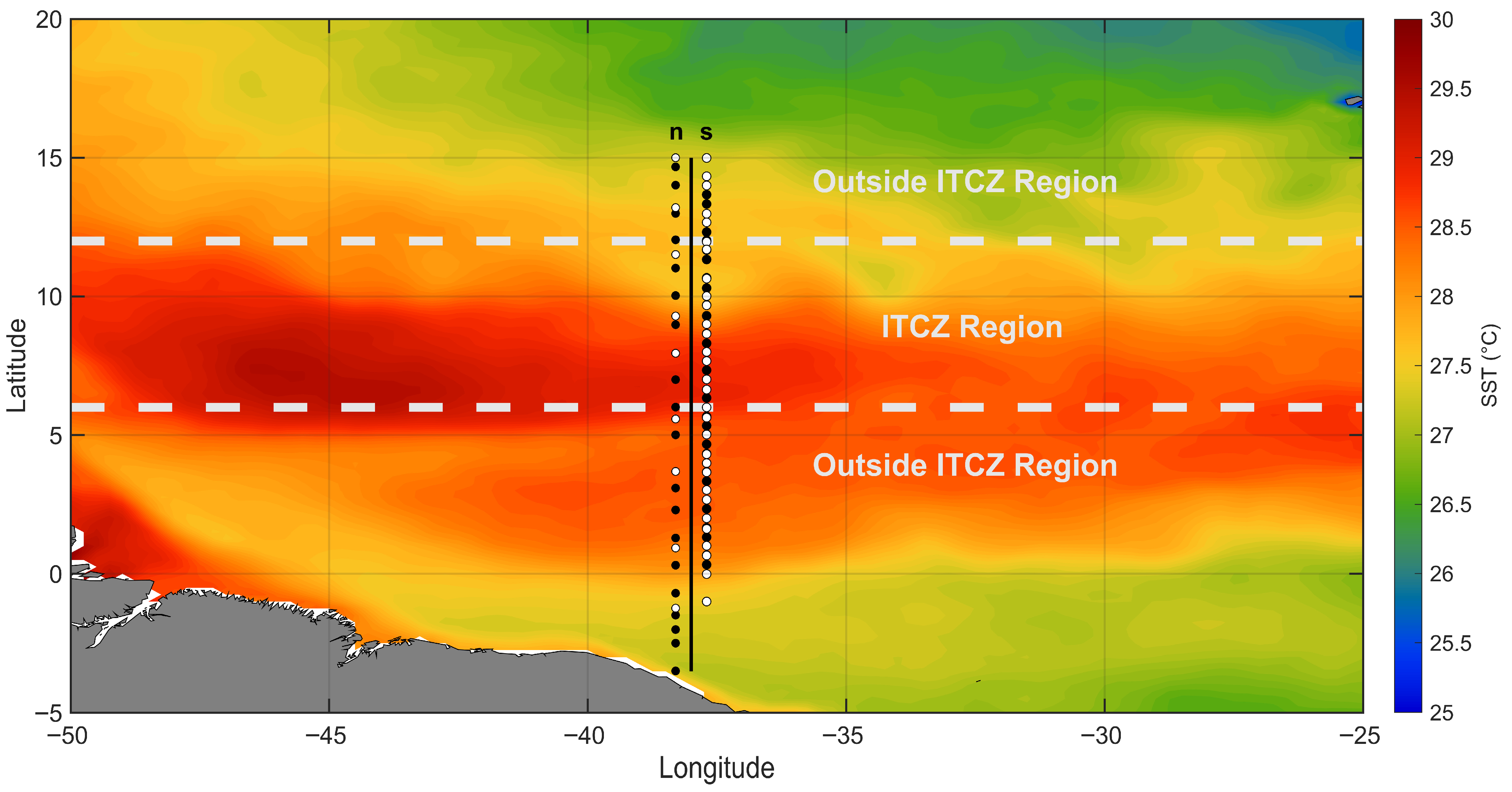
The study area is the WTAO, where in situ data were specifically collected along the 38° W meridian between the latitudes of 5° S and 15° N. The meridian was covered by the Brazilian Navy’s R/V Vital de Oliveira during the 3rd leg of the multidisciplinary field campaign PIRATA-BR-XVIII (PBR18-3). The campaign was conducted onboard R/V Vital de Oliveira, on which we collected both atmospheric (radiosonde) and oceanographic (XBT) data along two different paths: northbound (northward from 5° S) and southbound (southward from 15° N). The first path was held from 17 to 27 October 2018, while the second path was held from 27 October 2018 to 11 November 2018. Figure 1 presents the averaged SST field for this whole period with the radiosonde and XBT launching positions.

2.2. Radiosonde Data

A total of 47 radiosonde profiles were obtained along the 38° W meridian for assessing the characteristics of the atmosphere and for tracking the ITCZ position during the period of study.

Table 1. Radiosonde launching positions and dates for both northbound (R-1 to R-9) and southbound (R-10 to R-47) paths during the PBR18-3 campaign.

Radiosonde	Date	Latitude	Longitude	Radiosonde	Date	Latitude	Longitude
R-1	18 October 2018	−1.24	−38.00	R-25	1 November 2018	10.64	−38.01
R-2	19 October 2018	0.93	−38.00	R-26	1 November 2018	10.01	−38.02
R-3	20 October 2018	3.69	−38.00	R-27	1 November 2018	9.68	−38.01
R-4	21 October 2018	5.58	−38.00	R-28	2 November 2018	9.00	−38.01
R-5	22 October 2018	7.95	−38.00	R-29	2 November 2018	8.65	−39.00
R-6	23 October 2018	9.29	−38.00	R-30	2 November 2018	8.00	−38.02
R-7	24 October 2018	11.51	−38.00	R-31	3 November 2018	7.67	−38.00
R-8	25 October 2018	13.20	−38.00	R-32	3 November 2018	7.01	−38.00
R-9	26 October 2018	15.00	−38.00	R-33	4 November 2018	6.64	−37.99
R-10	26 October 2018	14.99	−38.01	R-34	4 November 2018	6.00	−38.03
R-11	27 October 2018	14.99	−37.99	R-35	4 November 2018	5.63	−38.01
R-12	27 October 2018	14.33	−38.00	R-36	5 November 2018	5.02	−38.00
R-13	27 October 2018	14.00	−37.00	R-37	5 November 2018	4.31	−37.96
R-14	28 October 2018	12.00	−38.01	R-38	5 November 2018	3.99	−37.95
R-15	28 October 2018	12.98	−38.06	R-39	5 November 2018	3.66	−37.98
R-16	29 October 2018	12.67	−37.95	R-40	6 November 2018	3.02	−38.01
R-17	30 October 2018	12.02	−37.71	R-41	6 November 2018	2.67	−38.02
R-18	30 October 2018	12.00	−37.77	R-42	6 November 2018	2.00	−38.00
R-19	30 October 2018	11.98	−37.37	R-43	7 November 2018	1.62	−38.02
R-20	30 October 2018	11.98	−37.91	R-44	7 November 2018	1.01	−37.99
R-21	31 October 2018	11.97	−37.75	R-45	7 November 2018	0.66	−38.00
R-22	31 October 2018	11.98	−37.82	R-46	8 November 2018	−0.01	−38.01
R-23	31 October 2018	11.97	−37.97	R-47	8 November 2018	−1.00	−38.00
R-24	31 October 2018	11.69	−38.01

describes the launching positions and dates of the radiosondes used here. Radiosondes 1 to 9 were launched during the ship’s northbound track, while radiosondes 10 to 47 were launched during the ship’s southbound track. The unequal number of launches was due to the work required to service the PIRATA buoys during the northbound path of the R/V Vital de Oliveira in the campaign. All radiosonde data were manually checked, and spurious data, found mainly at lower levels, were manually removed. When necessary, we used linear interpolation to fill in data along the vertical profile between different atmospheric heights.

Following Souza et al. [38], we built vertical profiles of some atmospheric variables to characterize the atmospheric conditions in both paths of the ship along the 38° W meridian during the PBR18-3 campaign. We used the air temperature (°C), the meridional component of the wind (m/s), and the atmospheric mixing ratio ($q_z$ in g/kg), which was calculated from original radiosonde data using Equations (1) and (2):

$$q_z={\displaystyle \frac{q_r\times 0.622\times e_z}{P-e_z}}$$

(1)

$$e_z=6.112\times e^{{\displaystyle \frac{17.67\times T_{air}}{T_{air}+243.5}}}$$

(2)

where $q_z$ is the mixing ratio (g/kg), $q_r$ is the relative humidity (%), P is the atmospheric pressure (hPa), $e_z$ is the water vapor pressure (hPa), and $T_{air}$ is the air temperature (K). Once calculated, the atmospheric mixing ratio ($q_z$) vertical profiles were plotted for both northbound ($q_{z}1$) and southbound ($q_{z}2$) paths of the ship’s route.

A vertical profile of the difference $q_{z}2$–$q_{z}1$ was also generated with the objective of estimating the major changes between the two paths as a proxy for the short-term ITCZ movement.

2.3. Outgoing Longwave Radiation Data

The ITCZ is a typical atmospheric convective system associated with a minimum value of OLR [39]. In this study, to describe an objective ITCZ band location, we used top-of-the-atmosphere OLR ERA5 re-analysis [40] data for the area of the WTAO (5° S–20° N, 25° W–50° W). The regions defined as the “ITCZ region” and “outside the ITCZ region” can be seen in Figure 1. The OLR data have a horizontal resolution of 0.25° × 0.25° and an hourly temporal resolution. The data were averaged for the period of both paths, and a single, temporal-averaged map was generated for each of the mean periods of both northbound and southbound paths. A map of the difference in ORL between the two periods was also generated, aiming to show the geographical position of the major changes in OLR for the period between the two paths.

2.4. Sea Water Temperature Data

The water temperature was measured in situ in both paths during the PBR18-3 campaign. We used Lockheed Martin Deep Blue XBTs. The sondes measure the sea water temperature at about every 0.6 m from the sea surface down to a depth of 760 m [41]. A total of 58 XBTs were used in this work, 19 of which were launched during the northbound path, and 39 were launched during the southbound path (

Table 2. XBT launching positions and dates for both northbound (XBT-1 to XBT-19) and southbound (XBT-20 to XBT-58) paths during the PBR18-3 campaign.

XBT	Date	Latitude	Longitude	XBT	Date	Latitude	Longitude
XBT-1	17 October 2018	−3.49	−36.40	XBT-30	31 October 2018	11.98	−37.73
XBT-2	18 October 2018	−2.50	−37.10	XBT-31	31 October 2018	11.98	−37.81
XBT-3	18 October 2018	−2.01	−37.42	XBT-32	31 October 2018	11.97	−37.99
XBT-4	18 October 2018	−1.49	−37.47	XBT-33	31 October 2018	11.67	−38.01
XBT-5	18 October 2018	−0.70	−37.78	XBT-34	1 November 2018	11.33	−38.01
XBT-6	19 October 2018	0.31	−37.87	XBT-35	1 November 2018	10.67	−38.01
XBT-7	19 October 2018	1.29	−37.99	XBT-36	1 November 2018	10.30	−38.00
XBT-8	19 October 2018	2.30	−37.98	XBT-37	2 November 2018	9.69	−38.01
XBT-9	20 October 2018	3.09	−37.98	XBT-38	2 November 2018	9.30	−38.00
XBT-10	21 October 2018	5.01	−37.94	XBT-39	2 November 2018	8.66	−37.99
XBT-11	21 October 2018	6.01	−37.97	XBT-40	2 November 2018	8.31	−37.98
XBT-12	21 October 2018	7.00	−38.02	XBT-41	3 November 2018	7.67	−38.00
XBT-13	23 October 2018	8.98	−38.01	XBT-42	3 November 2018	7.34	−38.00
XBT-14	23 October 2018	10.03	−38.01	XBT-43	3 November 2018	7.01	−38.00
XBT-15	24 October 2018	11.02	−38.00	XBT-44	4 November 2018	6.64	−37.99
XBT-16	24 October 2018	12.04	−37.96	XBT-45	4 November 2018	6.34	−37.99
XBT-17	25 October 2018	12.99	−38.01	XBT-46	4 November 2018	5.67	−38.01
XBT-18	25 October 2018	14.01	−38.02	XBT-47	4 November 2018	5.34	−37.99
XBT-19	25 October 2018	14.67	−38.01	XBT-48	5 November 2018	5.03	−38.00
XBT-20	27 October 2018	14.33	−38.00	XBT-49	5 November 2018	4.67	−37.98
XBT-21	27 October 2018	13.67	−38.00	XBT-50	5 November 2018	4.33	−37.96
XBT-22	28 October 2018	13.33	−38.01	XBT-51	5 November 2018	3.67	−37.98
XBT-23	28 October 2018	12.67	−38.06	XBT-52	6 November 2018	3.34	−38.00
XBT-24	29 October 2018	12.32	−38.06	XBT-53	6 November 2018	2.67	−38.02
XBT-25	29 October 2018	12.00	−37.93	XBT-54	6 November 2018	2.34	−38.01
XBT-26	30 October 2018	11.99	−37.61	XBT-55	7 November 2018	1.66	−38.02
XBT-27	30 October 2018	12.02	−37.70	XBT-56	7 November 2018	1.32	−38.02
XBT-28	30 October 2018	11.97	−37.91	XBT-57	7 November 2018	0.67	−38.00
XBT-29	30 October 2018	11.99	−37.76	XBT-58	7 November 2018	0.33	−38.01

). All data were manually checked, and spurious values were removed. We generated vertical profiles of water temperature to characterize the oceanographic conditions in both paths of the ship along the 38° W meridian during the PBR18-3 campaign.

To compare the distribution of observed sea water temperature with respect to the climatological distribution of the same variable along the 38° W meridian, we used data from the ECMWF’s Ocean Reanalysis System 5 (ORAS5) [42,43] and NOAA’s World Ocean Atlas 2023 (WOA23). As seen in

Table 3. Specifications of the open-access datasets used in this paper.

Dataset	Horizontal Resolution	Vertical Resolution	Period	Climatology
ORAS5	0.25° × 0.25°	75	October and November 2018	-
ORAS5	0.25° × 0.25°	75	October and November	1981–2010
WOA23	0.25° × 0.25°	57	October and November	1981–2010

, ORAS5 provided data for the months of October and November 2018, while we also computed climatological means (1981–2010) for the same months. WOA23 already provided climatological means for their monthly statistically averaged fields.

The vertical profiles were generated between a surface and a depth of 200 m and later compared to XBT profiles for both paths, between ~3.5° S (~0.5° N) and ~15° N for the northbound (southbound) path. It is important to note that ORAS5 only contains water potential temperature values, which were converted here to “normal” temperature using the Gibbs-SeaWater Oceanographic Toolbox [44], aiming to facilitate comparison between the different datasets.

During comparisons, specific levels of the XBT data were selected to match the available levels of both ORAS5 and WOA23. We selected data profiles that were the closest to the geographical coordinates of the XBT launching stations. In total, the first 31 (25) vertical levels of the ORAS5 (WOA23) datasets (representing the first 200 m of the water column) were used to perform three types of statistics: the bias, the root mean square error (RMSE), and linear regressions—as seen in Equations (3)–(5) below:

$$Bias={\displaystyle \frac{1}{z}}\sum _{i=0}^z(T_i^{dataset}-T_i^{XBT})$$

(3)

$$RMSE=\sqrt{{\displaystyle \frac{1}{z}}\sum _{i=0}^{z-1}{(T_i^{dataset}-T_i^{XBT})}^2}$$

(4)

$$R^2=1-{\displaystyle \frac{{\sum }_{i=0}^z{(T_i^{XBT}-{\widehat{T}}_i^{XBT})}^2}{{\sum }_{i=0}^z{(T_i-\overline{T^{XBT}})}^2}}$$

(5)

where $T_i^{dataset}$ and $T_i^{XBT}$ are the sea temperature at a vertical level $i$ from ORAS5 (or WOA23) and from XBT data, respectively; $\overline{T^{XBT}}$ is the mean XBT temperature over the matched $z$ levels; and ${\widehat{T}}_i^{XBT}=a+b{T}_i^{dataset}$.

SST averages for the period between the first and last days of the PBR18-3 campaign were also computed from ERA5 data [39] for the purpose of describing the general surface conditions of the study area. The data are originally available at hourly outputs, with a horizontal resolution of 0.25° × 0.25°.

2.5. Isothermal Layer (ILD) and Mixed Layer Depth (MLD)

There are a few known reliable methods to estimate the depth of the OML over the global ocean [1,25,45,46,47]. The main ones include searching for a layer in which a variable (usually temperature, salinity, density, or a combination of the three) is vertically homogenous. The issue with finding the right method for the WTAO concerns barrier layers (BL) [46,48,49], which form mainly due to salinity stratification, either from ITCZ-induced rainfall or from Amazon River discharge. The use of isothermal layer depths (ILDs) as a representation of the upper ocean mixing layer is known to overestimate the mixed layer depth (MLD) in regions where barrier layers are formed, as salinity plays an important role in these cases [48,50].

Because our oceanographic observational data is solely based on XBT probes, our analyses are limited to temperature-based algorithms, which would, in fact, correspond to the ILD instead of the MLD. Therefore, we applied a temperature threshold ($∆\mathrm{T}$ = 0.5 °C) to estimate the ILD for the XBT, ORAS5, and WOA23 datasets for comparative reasons. However, since both ORAS5 and WOA23 also provide salinity fields, we were able to apply a density threshold algorithm ($∆\rho$ = 0.5 kg·m⁻³) to estimate the MLD for these datasets.

Both algorithms used are based on identifying the first depth at which a given variable (temperature or density) departs from near-surface conditions by more than a prescribed threshold, starting from a reference depth of $z_0$ = 10 m (chosen to minimize the skin surface effect). The methodology follows the approach of Rabelo et al. [51], which adapted the framework proposed by Kara et al. [45] for use in XBT data. For consistency with previous studies, the threshold values were selected following Foltz et al. [1,25], who applied the same criteria to PIRATA moorings data along the 38° W meridian.

The temperature-based algorithm first identifies an isothermal layer, in which the temperature difference between consecutive depth levels does not exceed 10% of $∆\mathrm{T}$ (Equation (6)). The temperature at the bottom of the isothermal layer is taken as a new reference temperature ($T_{ref}$), used in Equation (7) to define the temperature at the top of the thermocline ($T_{th}$). The ILD is then defined as the depth of $T_{th}$. In contrast, the density algorithm does not explicitly search for an isopycnal layer. Instead, it defines the MLD as the first depth at which the density (${\rho }_{MLD}$) exceeds the reference density ($z_0$) by $∆\rho$ (Equation (8)).

$$\left|T_i-T_{i-1}\right|\le 0.1∆T$$

(6)

$$T_{th}=T_{ref}-∆T$$

(7)

$${\rho }_{MLD}={\mathrm{⍴}}_{z_0}+∆\mathrm{⍴}$$

(8)

2.6. Water Masses Analysis and Surface Currents Data

As mentioned above, ORAS5 and WOA23 climatologies also provided salinity fields for every profile close to the XBT launchings. These fields were used to plot potential temperature versus salinity (θ–S) diagrams using the Gibbs-SeaWater Oceanographic Toolbox [43,44]. The diagrams were used to describe the water mass distribution in four latitudinal bands along the 38° W meridian for the WTAO: (i) 5° S–0°; (ii) 0°–5° N; (iii) 5° N–10° N, and (iv) 10° N–15° N.

Surface ocean currents maps for the period of this study were obtained from the Ocean Surface Current Analyses Real-time (OSCAR) project [52]. OSCAR is an analysis product composed of both in situ and satellite data, offered at a daily frequency and a 0.25° × 0.25° spatial resolution. Data were averaged for the days that encompass both the northbound and southbound paths of the ship’s route and resampled to a 1.25° × 1.25° spatial average.

2.7. Synoptic-Scale Ocean–Atmosphere Interaction Analysis

The synoptic-scale ocean–atmosphere interaction processes that occurred along the 38° W meridian during the PBR18-3 campaign can be analyzed by combining the in situ synchronous measurements of the MABL and the ocean’s temperature taken by the radiosondes and XBTs. Ocean–atmosphere coupled profiles were plotted for both periods following the methodology described by Pezzi et al. [53] and recently used by Freitas et al. [54] and Faria et al. [29] for our study area. These profiles include the following variables: air temperature, water temperature (${\mathrm{T}}_{\mathrm{s}\mathrm{e}\mathrm{a}})$, and the meridional component of the wind. We also computed the difference between the ocean–atmosphere coupled variables along the 38° W meridian to assess the major changes in the study area during the period between the two paths of the ship.

Once the ITCZ’s position was defined using the OLR and radiosonde data, we followed the methodology described by Rabelo et al. [51] to study possible changes in the ILD and in the water temperature distribution along the 38° W meridian in the vicinity below the ITCZ for both paths of the ship.

2.8. Statistical Significance

To ensure the statistical significance and robustness of our results, we performed independent two-sample t-tests for all comparisons discussed throughout the article. These tests aimed to address two primary objectives: (1) to assess the variability inside and outside the ITCZ band region between the northbound and southbound paths of the ship’s route for each variable of interest (ILD, water temperature, air temperature, mixing ratio, OLR, and SST); and (2) to evaluate the differences between the in situ and ORAS5 and WOA23 data.

For the atmospheric variables, we conducted t-tests on $q_z$, $T_{air}$, and OLR across each study period. The in situ atmospheric profiles were evaluated vertically, while reanalysis (ERA5) data were averaged along the 38° W meridian. Similarly, oceanographic variables ($T_{sea}$, SST, and ILD) were vertically tested for each study period, using both in situ and climatologies. Additionally, we compared oceanic re-analysis fields directly against in situ observations to identify potential regional and temporal biases.

3. Results and Discussion

3.1. Atmospheric Conditions During the PBR18-3 Campaign

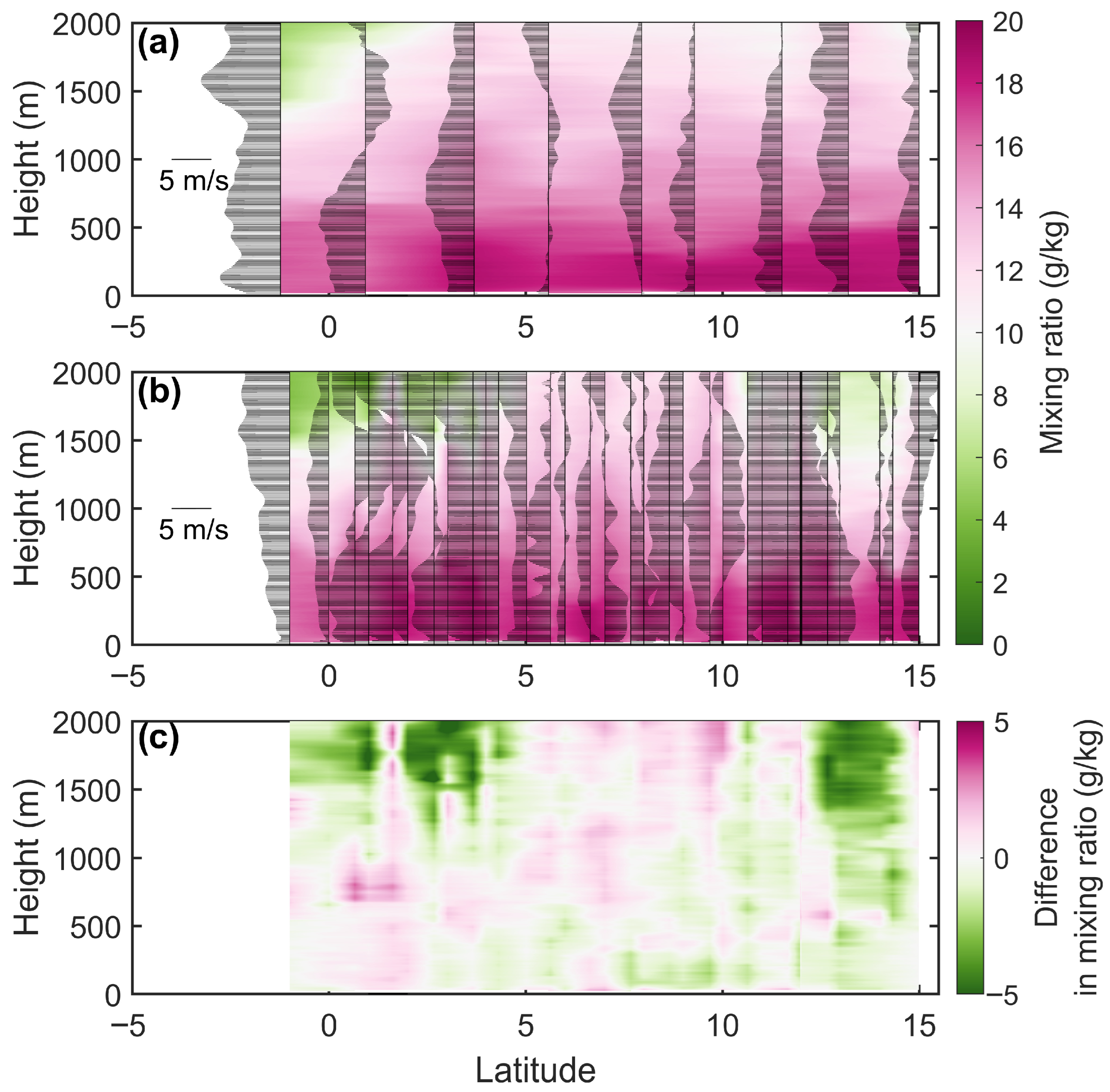
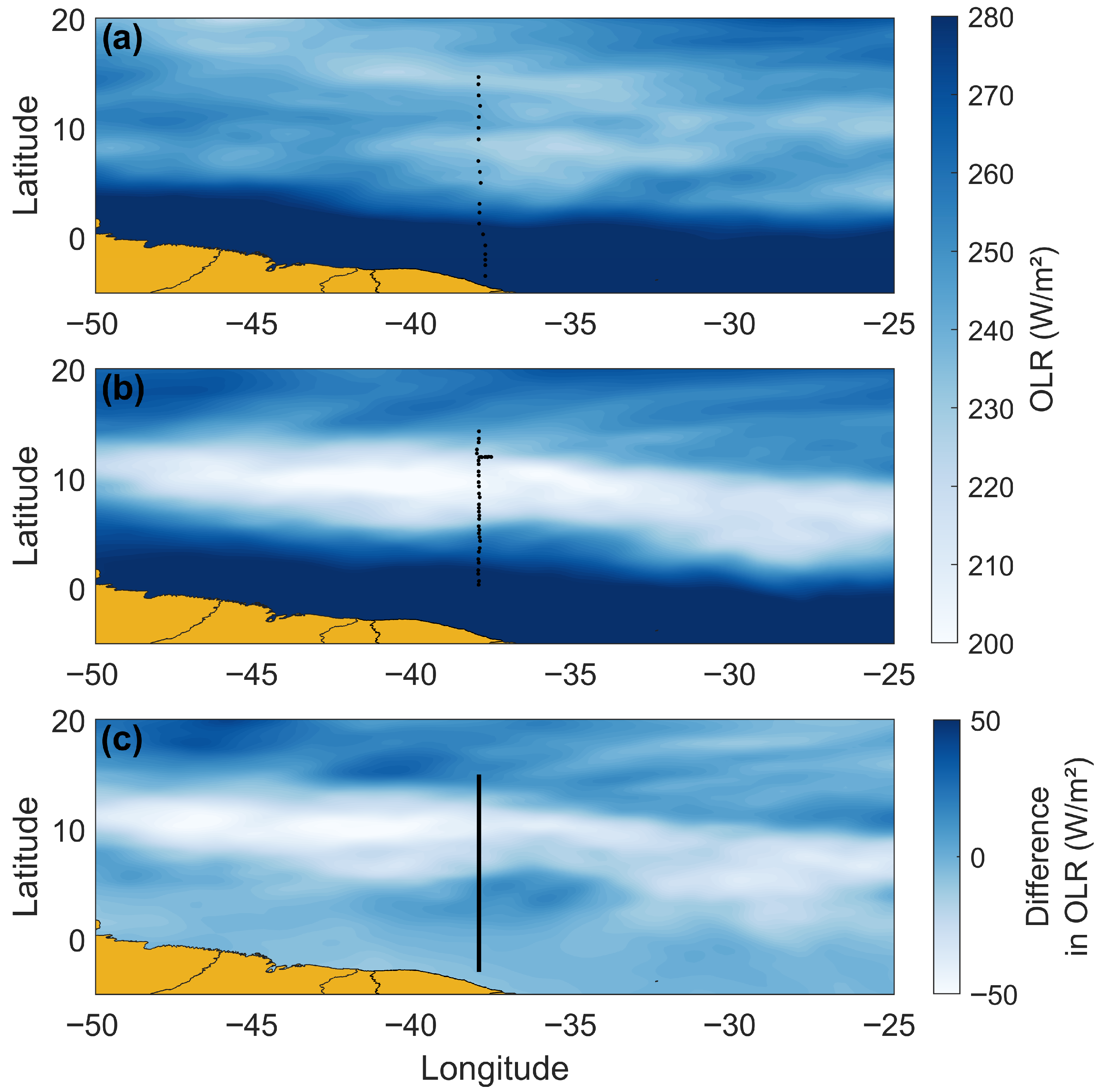
Before discussing the direct influence of the ITCZ on the upper WTAO, it is essential to define its meridional boundaries during the northbound and southbound paths of the campaign. Figure 2 presents the vertical distribution of atmospheric water vapor content ($q_z$) from the sea surface up to 2000 m along the 38° W meridian during both paths taken by the ship. The chosen height includes the entire marine atmospheric boundary layer (MABL). Figure 3 presents a map of the mean OLR in the WTAO during both northbound and southbound paths of the ship’s route in the PBR18-3 campaign. Low OLR values (~200 W/m²) are associated with the band of high cloudiness typical of the ITCZ.

When analyzing $q_z$ (Figure 2), we notice that in both the northbound and southbound phases, in the regions airside of the ITCZ, the MABL height ranges between 500 and 700 m, a value consistent with the findings of Ho et al. [55]. The MABL height can be inferred from the abrupt vertical change in atmospheric mixing ratio between the surface and upper heights. The ITCZ band width can be inferred from the homogeneity of the atmospheric mixing rate ($q_z$) from the sea surface up to 2000 m. During the first phase of our campaign, the southern boundary of the ITCZ is close to 1° S, while its northern boundary is north of 15° N (Figure 2a). During the second path, the ITCZ was confined within a latitude band of about 4° N to 12° N (Figure 2b).

The results show major differences in the change in $q_z$ above the MABL (~700 m) at the ITCZ’s southern and northern boundaries (Figure 2c), which is a consequence of higher convective activity at the ITCZ core during the southbound path ($q_{z}2$). Over a period of ~10 days, the $q_z$ outside the ITCZ limits changed on an order of about −5 g/kg (~42.2%), meaning the cloud cover outside the ITCZ boundaries diminished, and the upward branch of the Hadley cell became narrower between the two phases of the PBR18-3 campaign.

Figure 3 presents a map of the mean OLR in the WTAO during both northbound (a) and southbound (b) paths of the ship’s route in the PBR18-3 campaign. The difference in the mean OLR between the two periods can be seen in Figure 3c. A decrease in OLR of ~38 W/m² (~16%) indicates an intensification in cloud cover between 6° N and 13° N. Thus, over a 21-day period, the intensification of the northeast trades (see Figure 2b) contributed to a more confined convective activity and increased cloud cover between around 5° N and 12° N. A similar condition was observed by Serra and Houze Jr. [18] from wind and humidity profiles taken in the Eastern Pacific ITCZ, which were associated with atmospheric waves.

Based on the analysis of the $q_z$ and OLR (as well as their differences in time between both paths of the ship) seen in Figure 2 and Figure 3, we defined the mean position of the ITCZ in the WTAO between 6° N and 12° N. This band is considered here as “ITCZ region” (inITCZ), while anywhere lying outside of it will be called “outside ITCZ region” (outITCZ), as seen in Figure 1. The ITCZ boundaries are consistent with descriptions provided in previous works, which also discussed the short-term variability of the ITCZ using both model and observational data [17,18,20,22].

Table 4. Average values (plus standard deviations) for ${\mathrm{q}}_{\mathrm{z}}$, ${\mathrm{T}}_{\mathrm{a}\mathrm{i}\mathrm{r}}$, and OLR in the ITCZ and out of ITCZ regions during both northbound and southbound phases.

Zone	${\mathit{q}}_{\mathit{z}}$ (g/kg)		${\mathbf{T}}_{\mathbf{a}\mathbf{i}\mathbf{r}}$ (°C)		OLR (W/m2)
	Northbound	Southbound	Northbound	Southbound	Northbound	Southbound
inITCZ	12.40 ± 1.15	12.39 ± 1.55	18.52 ± 1.33	17.87 ± 1.49	237.37 ± 4.97	214.96 ± 9.61
outITCZ	11.84 ± 1.88	10.32 ± 2.75	17.90 ± 1.37	18.28 ± 1.20	268.44 ± 26.10	274.35 ± 19.79

presents the mean values of $q_z$, OLR, and air temperature ($T_{air}$) throughout the first 2000 m (height) for inITCZ and outITCZ. When comparing atmospheric variables across both regions, we found significant differences between the ITCZ and outside ITCZ regions (

Table A1. Differences and t-test results for each in situ variable for p < 0.05, including T-statistic, p-value, and upper and lower confidence intervals between the in situ data’s different regions and transects.

Variable	Comparison	Bias ± Std	T-Stat	p-Value	CI-Lower	CI-Upper
${\mathrm{q}}_{\mathrm{z}}$	Southbound × Northbound (inITCZ)	0.34 ± 0.80	10.55	9.04 × 10−26	0.28	0.40
	Southbound × Northbound (outITCZ)	−1.50 ± 1.59	−26.99	5.85 × 10−153	−1.62	−1.40
	Northbound × Northbound (inITCZ × outITCZ)	2.37 ± 1.38	44.41	0	2.51	2.75
	Southbound × Southbound (inITCZ × outITCZ)	2.26 ± 3.10	43.58	0	3.00	3.28
${\mathrm{T}}_{\mathrm{a}\mathrm{i}\mathrm{r}}$	Southbound × Northbound (inITCZ)	−0.69 ± 0.58	−17.26	6.65 × 10−65	−0.77	−0.61
	Southbound × Northbound (outITCZ)	0.45 ± 0.75	14.11	1.24 × 10−44	0.37	0.49
	Northbound × Northbound (inITCZ × outITCZ)	1.16 ± 0.60	19.52	1.58 × 10−80	0.88	1.07
	Southbound × Southbound (inITCZ × outITCZ)	−0.41 ± 1.06	−7.56	4.90 × 10−14	−0.42	−0.25
${\mathrm{T}}_{\mathrm{s}\mathrm{e}\mathrm{a}}$	Southbound × Northbound (inITCZ)	−0.08 ± 1.17	−0.60	0.55	−0.33	0.17
	Southbound × Northbound (outITCZ)	0.39 ± 1.50	−1.25	0.21	−0.34	0.07
	Northbound × Northbound (inITCZ × outITCZ)	−5.81 ± 4.23	−42.39	0	−5.73	−5.22
	Southbound × Southbound (inITCZ × outITCZ)	−2.85 ± 2.77	−23.93	6.94 × 10−122	−4.80	−4.07
OLR	Southbound × Northbound (inITCZ)	−24.63 ± 8.49	−12.67	6.44 × 10−17	−28.54	−20.72
	Southbound × Northbound (outITCZ)	3.05 ± 7.62	0.69	0.49	−5.69	11.79
	Northbound × Northbound (inITCZ × outITCZ)	−56.99 ± 9.19	−37.62	2.81 × 10−37	−60.04	−53.95
	Southbound × Southbound (inITCZ × outITCZ)	−74.96 ± 12.46	−37.86	1.40 × 10−41	−78.93	−70.99
SST	Southbound × Northbound (inITCZ)	0.06 ± 0.29	0.43	0.67	−0.22	0.34
	Southbound × Northbound (outITCZ)	0.10 ± 0.22	4.04	1.36 × 10−4	0.24	0.70
	Northbound × Northbound (inITCZ × outITCZ)	0.74 ± 0.48	8.43	1.74 × 10−10	0.72	1.18
	Southbound × Southbound (inITCZ × outITCZ)	−0.60 ± 0.05	−0.38	0.70	−0.52	0.35

). This sort of spatial and temporal variability represents a conclusive result that the ICTZ and its vicinity can undergo dramatic changes over short periods of time in our study region. We may now investigate how the OML and other properties responded to this change.

3.2. Oceanic Conditions During the PBR18-3 Campaign

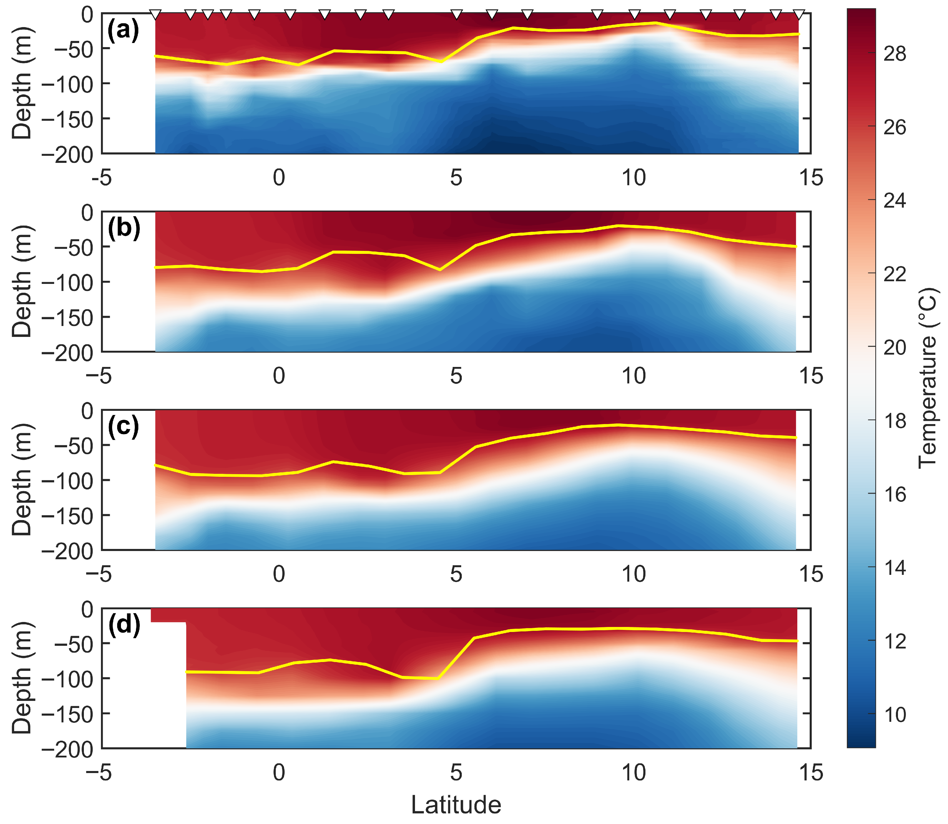
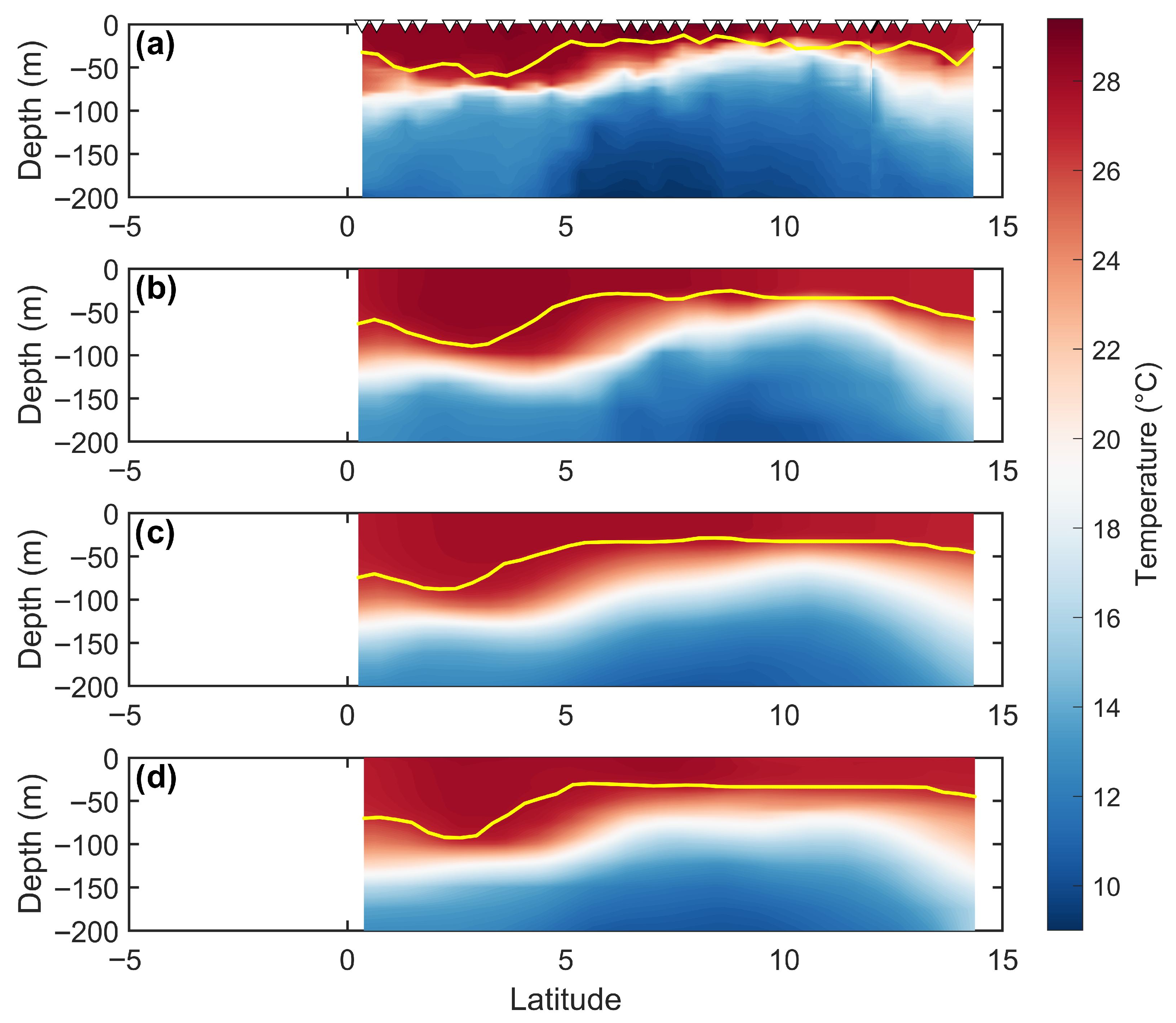
Figure 4 presents the vertical temperature transects at the 38° W meridian for the northbound path based on XBT, ORAS5, and WOA23 data, with the ILD shown as yellow lines. The ORA5 data shown is the October 2018 average and also the October climatology. All datasets exhibit a shoaling of the ILD between 5° N and 12° N, which corresponds to the Equatorial Divergence (ED). The ED is a region of shallower ILD, resulting from atmospheric low-level convergence (represented here by the ITCZ), Ekman pumping, and oceanic surface divergence [27,28]. The region is essential for primary productivity and ecological cycles, as the rich and cold undersurface water upwells and brings nutrients up to the euphotic zone. The ED in the WTAO is known to host diatoms [31,33], a phytoplankton class of unicellular algae associated with the Amazon River discharge, which makes the region a net sink of atmospheric CO₂ [34]. The nutrient enrichment of the WTAO is also maintained by Saharan dust (aerosol) deposition, transported westward by the trade winds [29]. In addition to increasing nutrients in the surface ocean, the Saharan dust can also reduce SST and ocean–atmosphere heat fluxes as well as deepen the OML through complex ocean–atmosphere feedback mechanisms [4].

Figure 4 shows that during the first path, the ILD became shallower north of 5° N, although the XBT data differed slightly when compared to other datasets; the ILD reached a minimum of ~14 m at ~11° N, whereas the other data indicated a deeper ILD.

As shown in Figure 2b, during the second path, the northeasterly trade winds begin to dominate the region north of 10° N. This forced the ILD to deepen south of 5° N, consequently shifting the southern boundary of the ED to about 3° S (Figure 5). This synoptic-scale change in the winds resulted in a significant (

Table A2. t-test statistics for p < 0.05, p-value, and upper and lower confidence intervals for all datasets (ORAS5, WOA23, and XBT) estimated ILDs.

Dataset	Comparison	T-Stat	p-Value	CI-Lower	CI-Upper
XBT	inITCZ × outITCZ (Northbound)	14.44	8.92 × 10−21	28.85	38.15
	inITCZ × outITCZ (Southbound)	7.97	3.75 × 10−9	14.90	25.12
	inITCZ (Northbound × Southbound)	0.14	0.89	−2.18	2.51
	outITCZ (Northbound × Southbound)	−4.15	1.03 × 10−4	−19.74	−6.90
ORAS5 monthly	inITCZ × Out of ITCZ (Northbound)	15.12	1.21 × 10−22	32.60	42.53
	inITCZ × Out of ITCZ (Southbound)	8.91	8.06 × 10−10	23.81	37.99
	inITCZ (Northbound × Southbound)	3.37	0.0016	1.71	6.82
	outITCZ (Northbound × Southbound)	−0.59	0.56	−10.58	5.78
ORAS5 climatology	inITCZ × Out of ITCZ (Northbound)	12.45	1.74 × 10−18	37.38	51.68
	inITCZ × Out of ITCZ (Southbound)	7.60	3.23 × 10−8	20.62	35.85
	inITCZ (Northbound × Southbound)	1.84	0.077	−0.32	5.87
	outITCZ (Northbound × Southbound)	−2.74	0.0080	−23.38	−3.67
WOA23 climatology	inITCZ × outITCZ (Northbound)	13.18	5.88 × 10−17	36.58	49.79
	inITCZ × outITCZ (Southbound)	6.40	7.78 × 10−7	18.52	35.87
	inITCZ (Northbound × Southbound)	4.95	2.07 × 10−5	1.36	3.25
	outITCZ (Northbound × Southbound)	−2.57	0.013	−24.36	−3.02

) ILD variability in outITCZ with respect to inITCZ, especially evident in our XBT data.

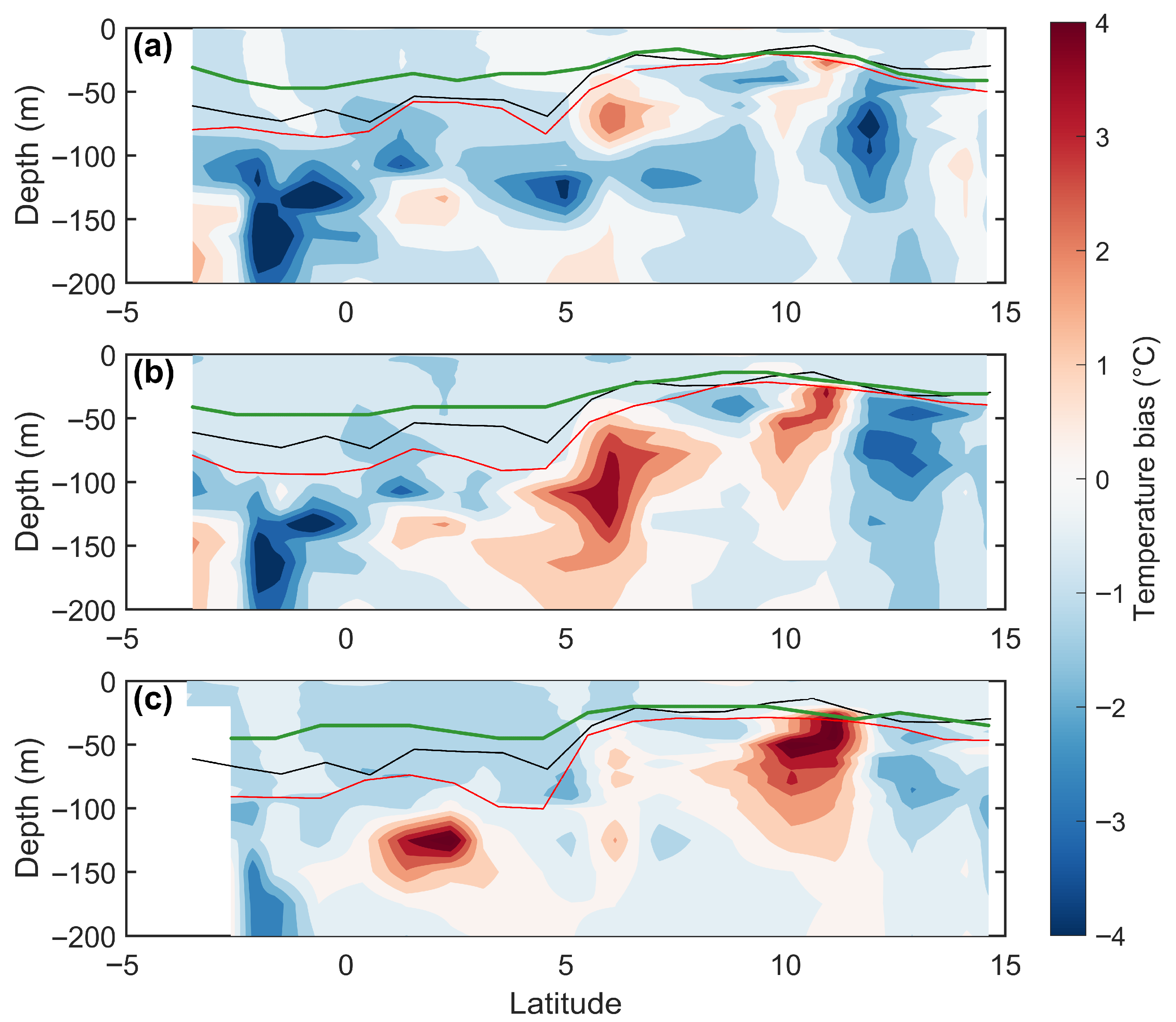
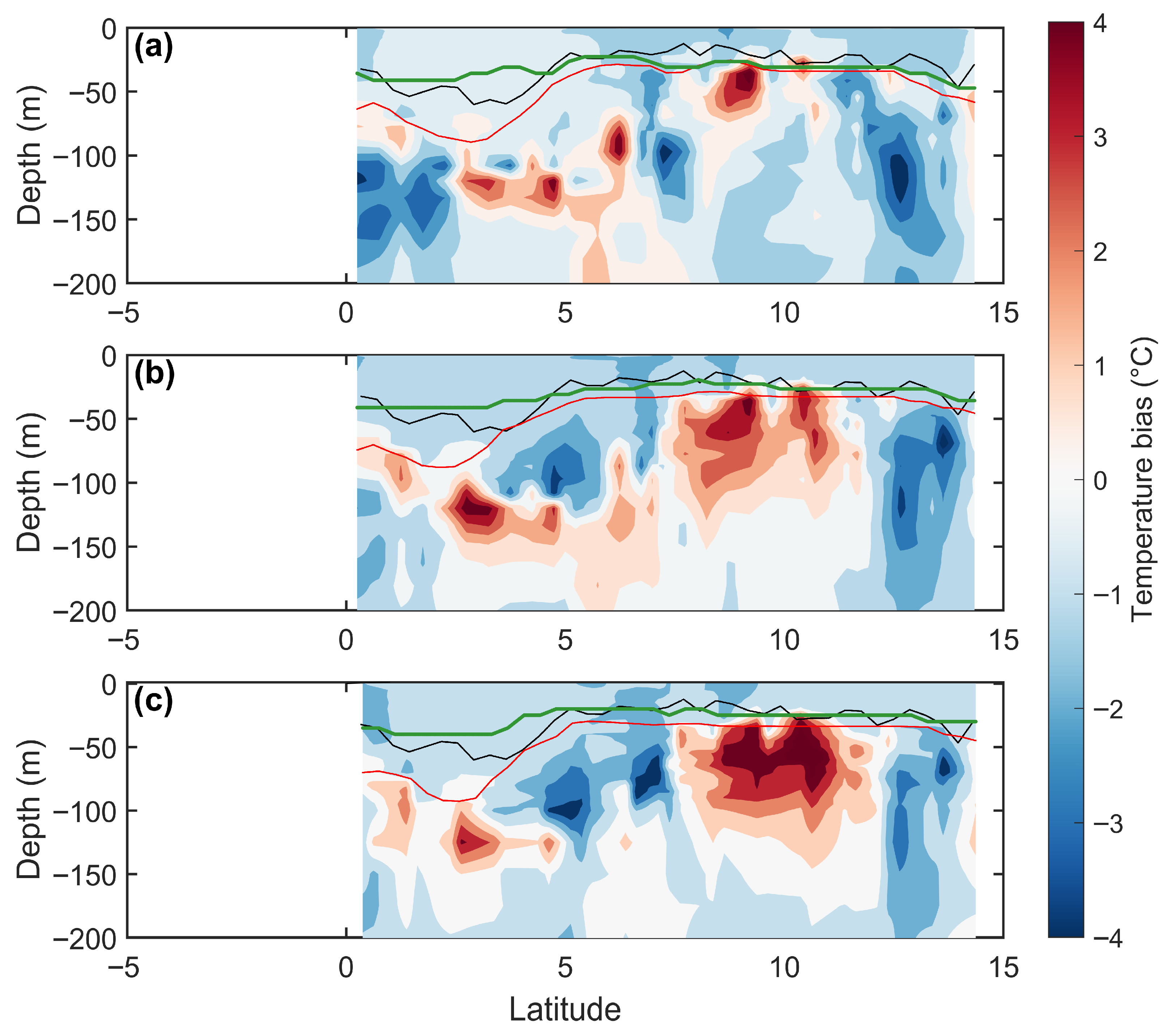
Figure 6 and Figure 7 present, respectively, the vertical water temperature difference (biases) transects obtained for the northbound and southbound tracks. The biases were computed as the water temperature difference between the ORAS5 and WOA23 with respect to the observational data. All datasets generally exhibit a colder water column with respect to observational data, particularly at the surface, with negative biases reaching −2 °C. The largest positive biases are seen below the ILD, near the depth of the 20 °C isotherm, and at the meridional boundaries of the ED (Figure 6 and Figure 7). The temperature-difference transects reveal consistent spatial patterns in the discrepancies between the XBT profiles and the three datasets. All datasets represent the ILD as being systematically deeper than that indicated by the XBT-derived ILD (

Table A3. t-test statistics for p < 0.05, p-value, and upper and lower confidence intervals between ORAS5 and WOA23 data and the XBT data for estimated ILD.

Transect	Comparison	T-Stat	p-Value	CI-Lower	CI-Upper
Northbound	ORAS5 monthly × XBT (inITCZ)	−4.92	1.20 × 10−5	−9.29	−3.90
	ORAS5 monthly × XBT (outITCZ)	−3.41	9.54 × 10−4	−16.87	−4.46
Southbound	ORAS5 monthly × XBT (inITCZ)	−9.86	1.24 × 10−13	−12.87	−8.52
	ORAS5 monthly × XBT (outITCZ)	−5.21	3.95 × 10−6	−29.91	−13.25
Northbound	ORAS5 climatology × XBT (inITCZ)	−4.72	3.33 × 10−5	−11.33	−4.52
	ORAS5 climatology × XBT (outITCZ)	−4.84	6.23 × 10−6	−26.76	−11.16
Southbound	ORAS5 climatology × XBT (inITCZ)	−11.70	1.05 × 10−13	−12.36	−8.70
	ORAS5 climatology × XBT (outITCZ)	−4.27	9.74 × 10−5	−27.60	−9.92
Northbound	WOA23 climatology × XBT (inITCZ)	−10.08	4.48 × 10−12	−11.04	−7.34
	WOA23 climatology × XBT (outITCZ)	−4.83	6.98 × 10−6	−26.67	−11.09
Southbound	WOA23 climatology × XBT (inITCZ)	−13.06	4.20 × 10−14	−13.09	−9.56
	WOA23 climatology × XBT (outITCZ)	−3.83	4.34 × 10−4	−28.27	−8.75

), with the offset persisting along the entire section. This deeper ILD is accompanied by warm anomalies within the upper thermocline, particularly between 5° and 10° N, where the ORAS5 and WOA23 climatologies reach more than +3 °C relative to the observations. Moreover, the ILD in inITCZ is also significantly different from outITCZ (Table A2).

The water temperature differences found indicate that the datasets partially capture the vertical structure of the upper-ocean water masses but still misrepresent the depth and intensity of their cores, with warm biases frequently emerging above ~50–80 m within the Tropical Water layer and cold biases strengthening between ~100–200 m, where the upper portion of the South Atlantic Central Water (SACW) is expected. The systematic displacement of the ILD further highlights structural inconsistencies relative to the XBT profiles, consistent with known biases in tropical Atlantic re-analyses [40,41].

On average, as seen in

Table 5. Average ILD and standard deviations (in meters) estimated from XBT, ORAS5, and WOA23 data during the northbound (October) and southbound (November) paths in the ITCZ and outside ITCZ regions.

Dataset	Zone	Northbound (October)	Southbound (November)
XBT	inITCZ	−20.2 ± 4.6	−21.83 ± 5.23
	outITCZ	−51.97 ± 17.69	−41.4 ± 12.91
ORAS5 monthly	inITCZ	−26.81 ± 5.24	−32.0 ± 3.25
	outITCZ	−63.03 ± 18.72	−64.43 ± 16.87
ORAS5 climatology	inITCZ	−28.79 ± 7.91	−32.44 ± 1.97
	outITCZ	−69.47 ± 25.64	−60.77 ± 19.67
WOA23 climatology	inITCZ	−29.88 ± 1.23	−32.65 ± 1.33
	outITCZ	−70.0 ± 25.35	−61.02 ± 21.19

, the difference between the estimated ILD for the ORAS5 and WOA23 datasets and the XBT data ranges from 6.6 to 8.8 m (11.6 to 18.03 m) deeper in inITCZ (outITCZ) for the first phase (Figure 6). For the second phase (Figure 7), the difference ranges from 10.61 to 10.82 m (19.37 to 23.03 m) deeper than the XBT-estimated ILD in inITCZ (outITCZ). Compared with October (Figure 6), the November temperature-bias distribution (Figure 7) becomes more vertically structured and meridionally coherent. Warm anomalies intensify and deepen between ~80–150 m, most notably in WOA23, while cold biases expand between ~100–200 m, especially south of the equator. The mismatch between the ILD from the re-analyses and the XBT persists and becomes more evident in November, reflecting the strengthening of subsurface signals. Overall, the November pattern shows a clearer and more organized bias structure than in October. According to Karmakar et al. [56], ORAS4 (predecessor of ORAS5) and three other oceanic re-analyses present a negative bias with respect to observations of the ocean’s mixed layer stability, a measure that indicates an excess mixing in the ocean from climatological data.

As expected, the mean MLD is shallower than the ILD in both ORAS5 and WOA23, resulting in a well-defined barrier layer thickness (BLT) south of the ED (35.70–41.51 m). The period of study is in austral spring, characterized by the North Equatorial Counter Current (NECC), which extends the Amazon River plume eastward during austral spring [25,30,48]. This region is also where the XBT-derived ILD exhibits the strongest decoupling from the estimated MLD.

From the southern boundary of the ED to the northern end of the section, the BLT thins considerably, with average values between 5.86 m and 10.31 m. These values are close to the BLT depicted in the results of Saha et al. [48], with BLT values below 10 m north of the NECC, and confirm the authors’ claim that sometimes ocean dynamics can be the sole driver of BLT variability, without the main influence of the ITCZ’s freshwater input. Thus, in the ED region, the ILD method showed good agreement and can be applied to estimate the MLD.

Zuo et al. [43] highlighted the improvements in the ORAS5 dataset compared to its previous versions, emphasizing the difficulty of oceanic re-analysis datasets to accurately represent the WTAO. As this region is dominated by eddies exported from the North Brazil Current (NBC), the importance of an observing system for the Tropical Atlantic is paramount [9,23,24]. The differences between our observational data and the other datasets may also indicate a misrepresentation of the current systems in the climatologies, especially the NBUC core [42], which feeds the NBC. All ocean re-analyses currently available struggle to accurately represent the NBUC due to limitations in data assimilation and the scarcity of observational data [43,44]. Other important currents that could be misrepresented are the Equatorial Undercurrent (EUC), at around 5° N, and the North Equatorial Undercurrent (NEUC), at around 10° N, which mainly transport SACW below the thermocline [57].

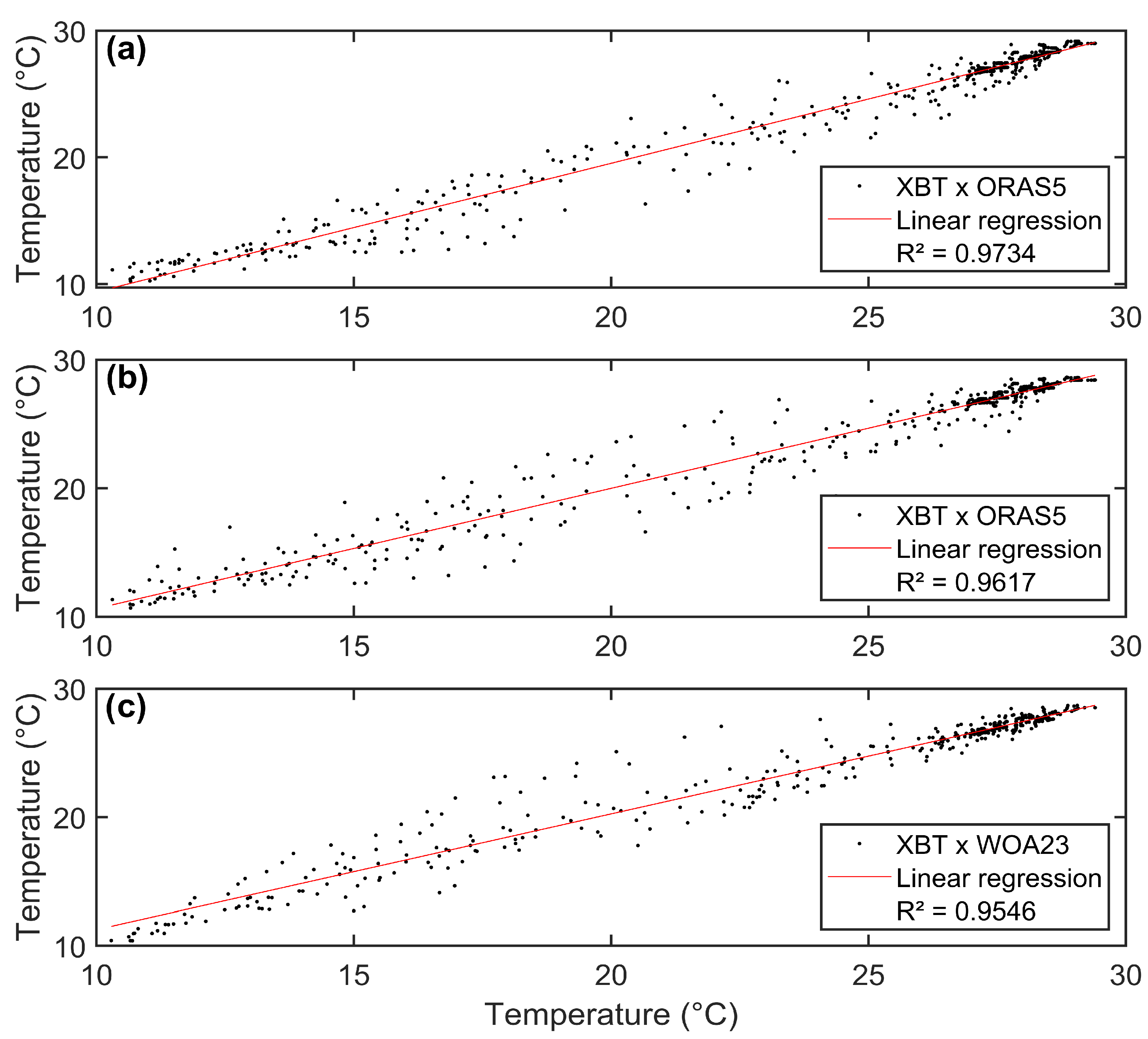
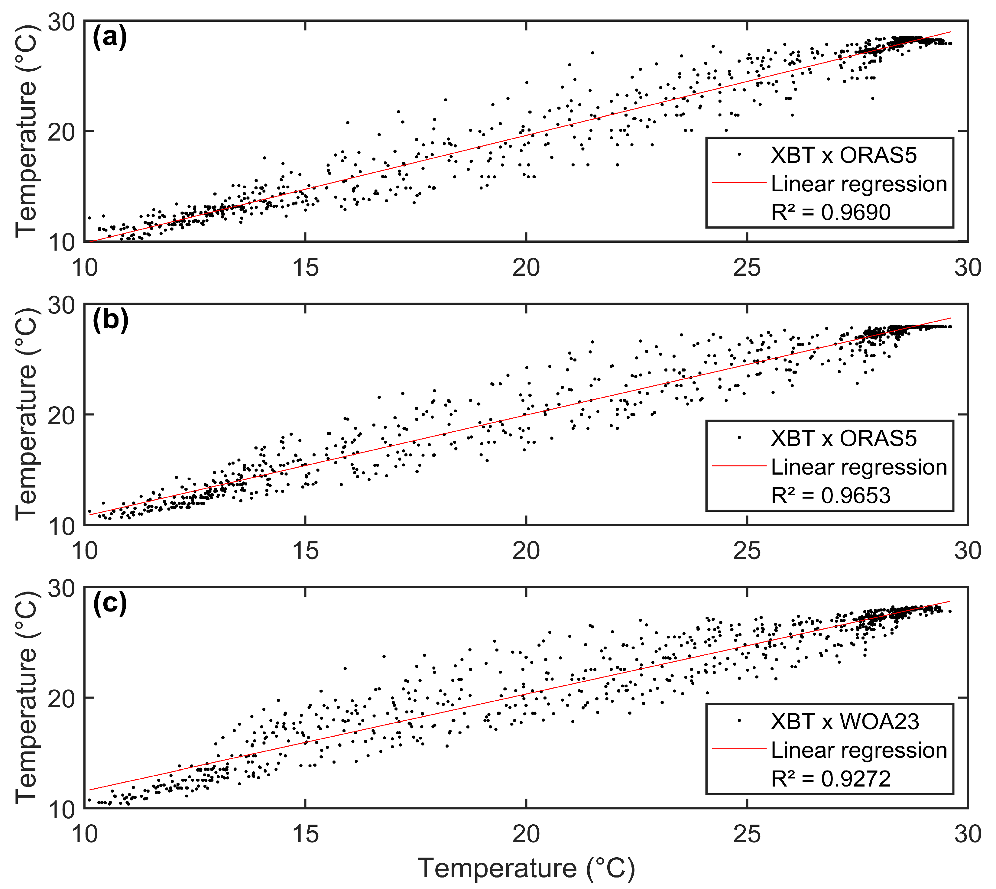
In general, the highest water temperature biases between observational and climatological data are found in the ED region, around the ILD. As such, all average biases are found to be significant, except for the comparison between the XBT and ORAS5 monthly data for the ITCZ region during the northbound phase (

Table 6. Average biases (±standard deviation), with t-test statistics for p < 0.05, p-value, upper and lower confidence intervals, and RMSE between ORAS5, WOA23, and the XBT data for the northbound phase of the PBR18-3 campaign.

Database	Zone	Bias (°C)	RMSE	T-Stat	p-Value	CI-Lower	CI-Upper
ORAS5 monthly	inITCZ	−0.17 ± 0.78	0.80	−6.05	2.22 × 10−9	−0.23	−0.11
	outITCZ	−0.47 ± 0.76	0.89	−23.67	4.75 × 10−105	−0.51	−0.43
ORAS5 climatology	inITCZ	0.25 ± 1.03	1.06	6.78	2.30 × 10−11	0.18	0.32
	outITCZ	−0.47 ± 0.81	0.94	−22.24	1.43 × 10−94	−0.51	−0.43
WOA23 climatology	inITCZ	0.70 ± 1.28	1.46	13.69	1.78 × 10−37	0.60	0.80
	outITCZ	−0.50 ± 0.67	0.84	−24.79	2.29 × 10−108	−0.54	−0.46

and

Table 7. Average biases (±standard deviation), with t-test statistics for p < 0.05, p-value, upper and lower confidence intervals, and RMSE between ORAS5, WOA23, and the XBT data for the southbound phase of the PBR18-3 campaign.

Database	Zone	Bias (°C)	RMSE	T-Stat	p-Value	CI-Lower	CI-Upper
ORAS5 monthly	inITCZ	−0.03 ± 1.27	1.27	−0.78	0.43	−0.12	0.05
	outITCZ	−0.63 ± 0.90	1.09	−20.31	7.15 × 10−75	−0.69	−0.57
ORAS5 climatology	inITCZ	−0.43 ± 1.00	1.09	−12.99	1.69 × 10−35	−0.50	−0.37
	outITCZ	−0.32 ± 0.76	0.82	−12.15	2.22 × 10−31	−0.37	−0.27
WOA23 climatology	inITCZ	0.50 ± 1.93	2.00	7.03	4.94 × 10−12	0.36	0.65
	outITCZ	−0.58 ± 0.86	1.04	−17.62	1.99 × 10−57	−0.65	−0.52

). Nevertheless, Figure 8 and Figure 9 show that all datasets exhibit a strong linear correlation with the in situ data, with r² values exceeding 0.9 in all cases. The lowest r² is found between the WOA23 and XBT data, possibly due to the extensive interpolation processes used in the analysis, which is constructed from millions of in situ observations historically taken [58].

Although all datasets are well correlated with in situ observations, their use as input for forecasting models should be carried out with caution, considering their ability to reproduce the oceanic characteristics of the WTAO. This is particularly critical, as this region is dominated by the NBC rings, which are closely linked to the AMOC [59,60,61]. Additionally, the studied transects are part of the main development region, where many famous tropical storms [24,62,63,64] have either formed or intensified before causing havoc and severe socio-economic damage in Central and North America, as well as the ocean wave climate in the Brazilian Equatorial Margin [65]. This adds further scientific interest to the WTAO and underscores the importance of accurately representing its dynamics [43,66].

3.3. Water Masses and Surface Currents

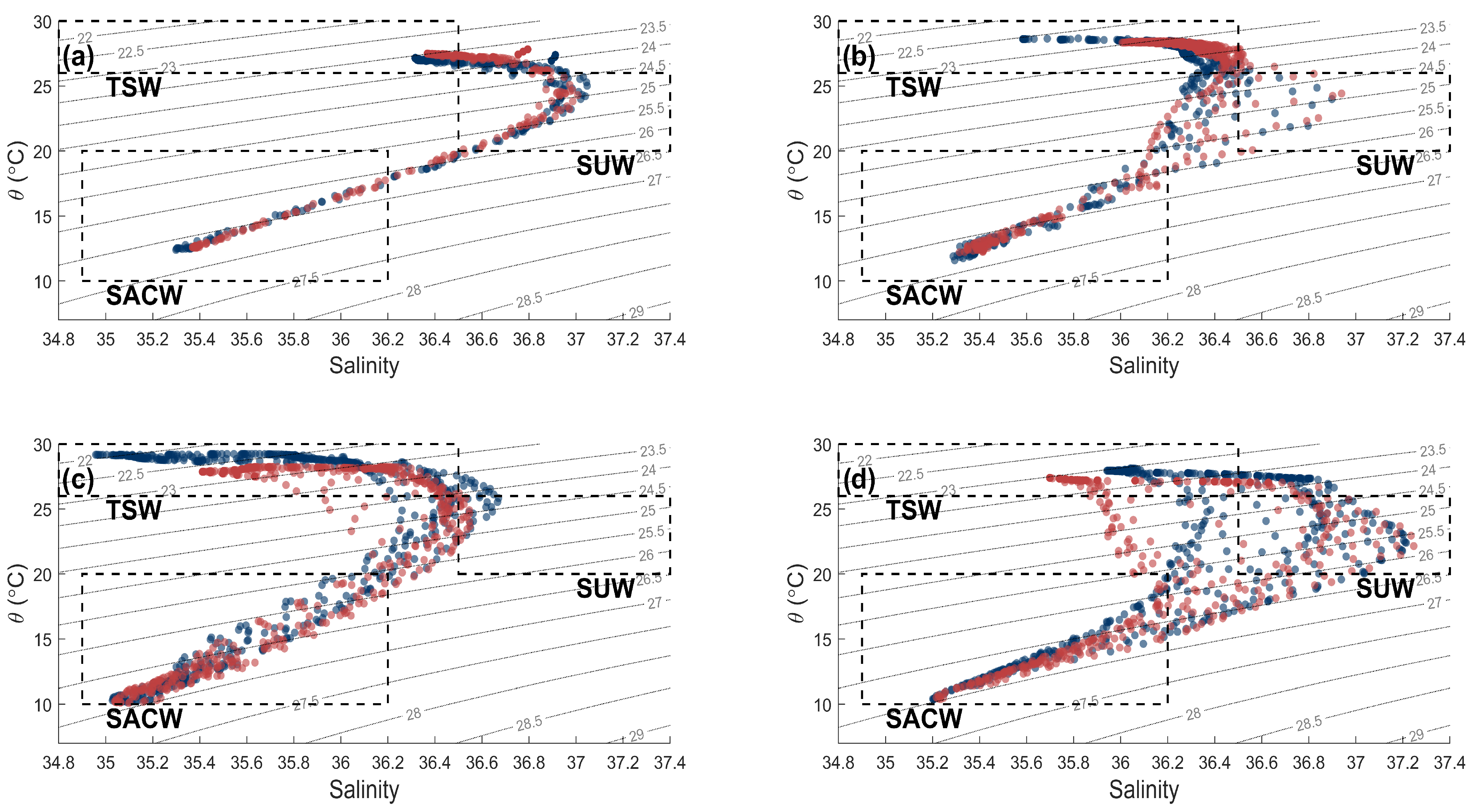
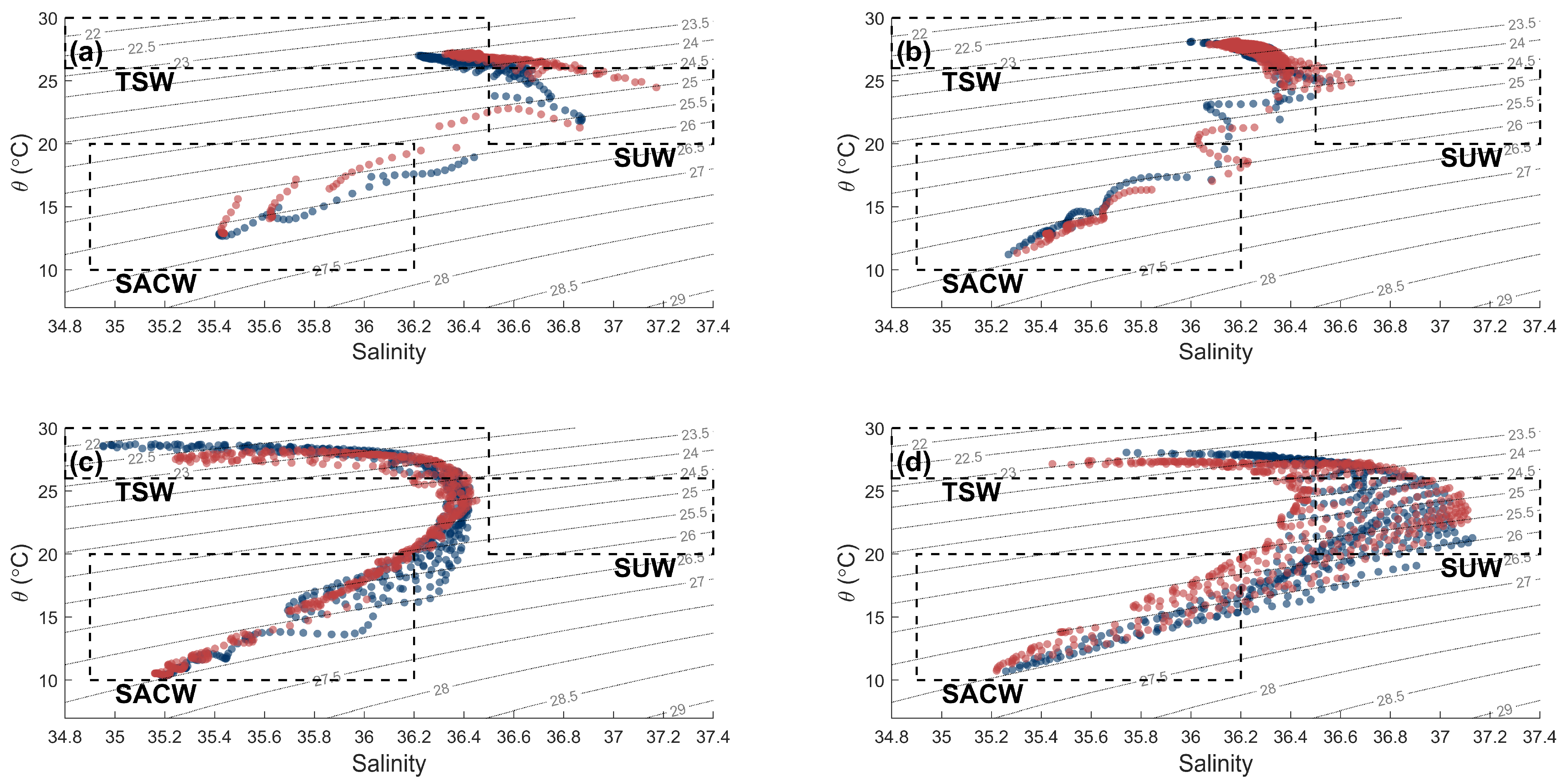
Figure 10 and Figure 11 illustrate the water masses structure of the upper 200 m along the 38° W path of the PBR18-3 campaign, based on ORAS5 and WOA23 climatologies, separated into four latitudinal bands. Based on the findings of Costa da Silva et al. [67], we identified three water masses: Tropical Surface Water (TSW), Subtropical Underwater (SUW), and SACW. The TSW is characterized by temperatures above 26 °C and salinities lower than 36.5. Directly below the TSW lies the SUW, with temperatures ranging from 20 °C to 26 °C and salinities exceeding 36.5. The SACW is below the SUW, with temperatures between 10 °C and 20 °C and salinities between 34.9 and 36.2. As a result, the TSW represents the OML of the study area, above the SUW, which is separated from the SACW by the 20 °C isotherm [59].

At the surface, above 100 m, the southernmost band (5° S–0°) exhibits the narrowest ranges of temperature, salinity, and density, indicating that it lies outside the direct influence of the ITCZ. The 0°–5° N band, however, may not be directly below the ITCZ, but it is still affected by the surrounding convective activity, contributing to surface cooling and freshening (Figure 10b and Figure 11b). For this very reason, the two northern bands (5° N–10° N and 10° N–15° N) display the broadest ranges of temperature, salinity, and density. Lower surface θ–S pairs are evidence of the ITCZ-associated precipitation and the presence of the ED, which brings colder, more saline waters below a shallow OML, and inhibits the presence of the SUW, which is the most saline water mass in the 38° W meridian [67].

From 100 m to 200 m, we can observe the behavior of the 20 °C isotherm. Broad ranges of temperature, salinity, and density highlight the presence of the SACW, typically lying between 150 m and 500 m below the surface [67]. The upward movement of the SACW, transported by the NBC [59,60,61], scatters the θ–S pairs at around 120 m. This becomes more evident closest to the ED and ITCZ, especially in the ORAS5 data. Below 100 m, WOA23 appears to be under-represented, possibly due to a lack of observational data [43,44], and the SUW is not seen at the ITCZ-ED region (Figure 11c). Weaker vertical gradients are observed in the two northern bands, as a shallow OML means the colder, more saline ED dominates the water column.

In both datasets (ORAS5 and WOA23), the salinity ranges broaden from October to November (Figure 10 and Figure 11). November marks the transition between austral spring and summer, which suggests the beginning of the ITCZ’s southward migration. Thus, the northeast trade winds are intensified, and the precipitation maxima are expected to shift southward [3,5,68], as the surface Ekman pumping is enhanced and the ED transports more cold, saline waters into the subsurface.

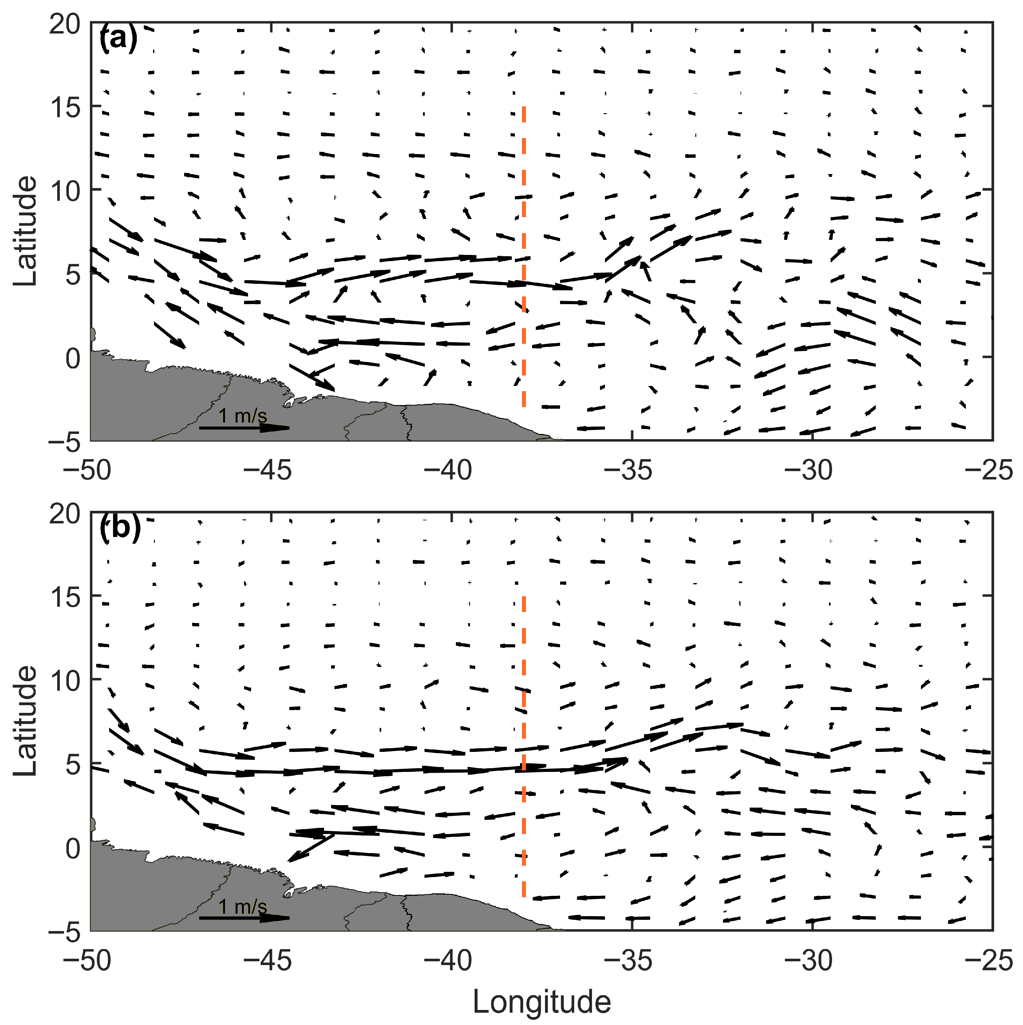
Figure 12 illustrates the North Equatorial Counter Current (NECC), at about 5° N, as a zonal current of about 1 m/s that is fed by the retroflection of the NBC at around 5° N, 52° W during austral spring [35,36,37]. North of the NECC, the surface currents are very weak, as the ITCZ is in its northernmost position, where weak surface winds prevail below it. During the study period, a strong ED is also expected [28]. During the northbound phase of the PBR18-3 campaign, tropical instability waves (TIWs) can be spotted moving westward due to the horizontal shear between the eastward NECC and the westward central branch of the South Equatorial Current (cSEC), forcing anticyclonic activity at the oceanic surface [69]. The TIWs seem to have crossed the 38° W meridian during the northbound phase at around 5° N and then moved away from the transect during the southbound phase.

Liu et al. [70] have shown that in the event of TIWs in the Pacific cold tongue, the mixing within the mixed layer (above the thermocline) is enhanced. Fang et al. [71] justify that TIWs are associated with the deepening and shoaling of mixing, and the seasonal variability of NBC rings modulates the thickness of the OML [72]. Thus, the TIWs can be the origin of the observed temperature anomalies below the OML at around 5° N, as the associated anticyclonic movement has been found to modulate mixing in the water column strongly [71]. Such a hypothesis should be further investigated.

3.4. Synoptic-Scale Ocean–Atmosphere Interaction

During the northbound phase of the PBR18-3 campaign, the southeast trades dominated the lower atmosphere, as the ITCZ was in its northernmost position [3,5,73,74], which we previously defined as between 6° N and 12° N. The vertical temperature sections shown in Figure 13 highlight the influence of the ED on ocean stratification and its synoptic variability. Directly beneath the ITCZ, colder subsurface waters are upwelled, which shoals both the OML and the thermocline.

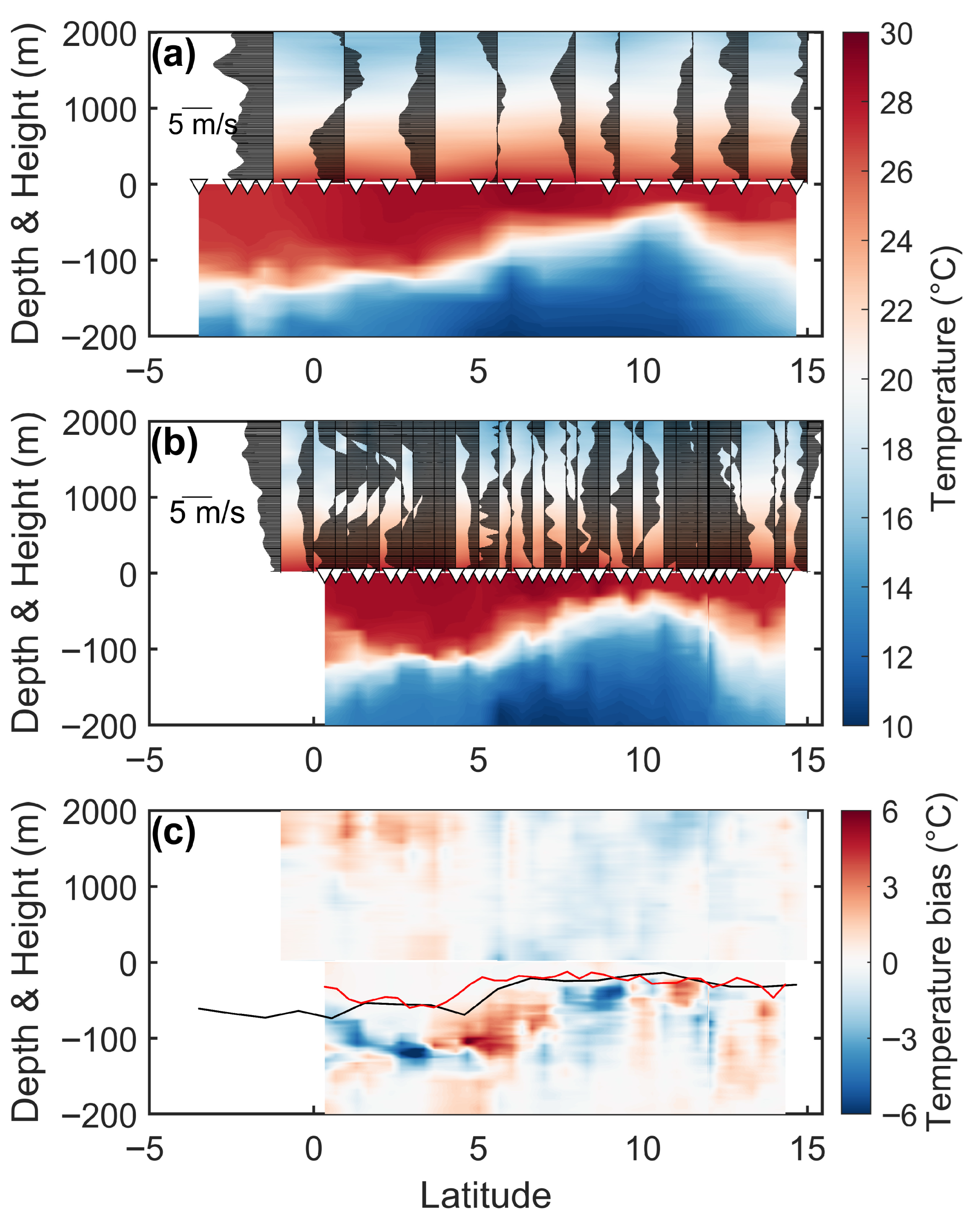
During the northbound path (Figure 13a), the ILD depth for inITCZ was 20.20 ± 4.60 m, while a deeper ILD was estimated for outITCZ (51.97 ± 17.69—Table 5). The ED appeared slightly displaced northward, with shallower ILD values around 11° N (Figure 13a), likely due to the predominance of the southeast trades, which push the ED northward through enhanced mixing within the OML. During the southbound path (Figure 13b), the ILD was 21.83 ± 5.23 m deep in inITCZ and 41.40 ± 12.91 m deep in outITCZ (Table 5). The onset of the northeast trade winds opposed the observed northward displacement of the ED, shifting it southward and extending the southern boundary of the ED south of 5° N (Figure 11). This shift shoaled the average OML in outITCZ, highlighting the ocean’s ability to respond rapidly to synoptic-scale atmospheric changes, despite its relatively high inertia.

Between both ship phases, the ITCZ became more concentrated within 6° N–12° N, leading to increased precipitation within this band. As a result, atmospheric temperatures decreased by ~1.7 °C (Figure 13c) within the ITCZ region, while the decrease in cloudiness (and precipitation) resulted in an increase in atmospheric temperature outside the ITCZ by about 2 °C. Between 7° N and 10° N, the waters just below the ILD cooled (3–5 °C), owing to the southward shift of the ED and the intensification of the northeasterlies.

South of the ED shift, around the depth of the 20 °C isotherm, water temperatures increased by 3–6 °C (Figure 13c), whereas they were expected to cool as a response to the OML shoaling. This warming could reflect the following: a compensatory mechanism in the ocean, adjusting to rapid changes in the northern ED region; an error in the ILD estimation method; or the impact of the TIWs that were spotted around the 38° W meridian during the northbound path. Overall, the general trend observed was that water column cooling corresponded with OML shoaling, while warming was associated with a thicker OML.

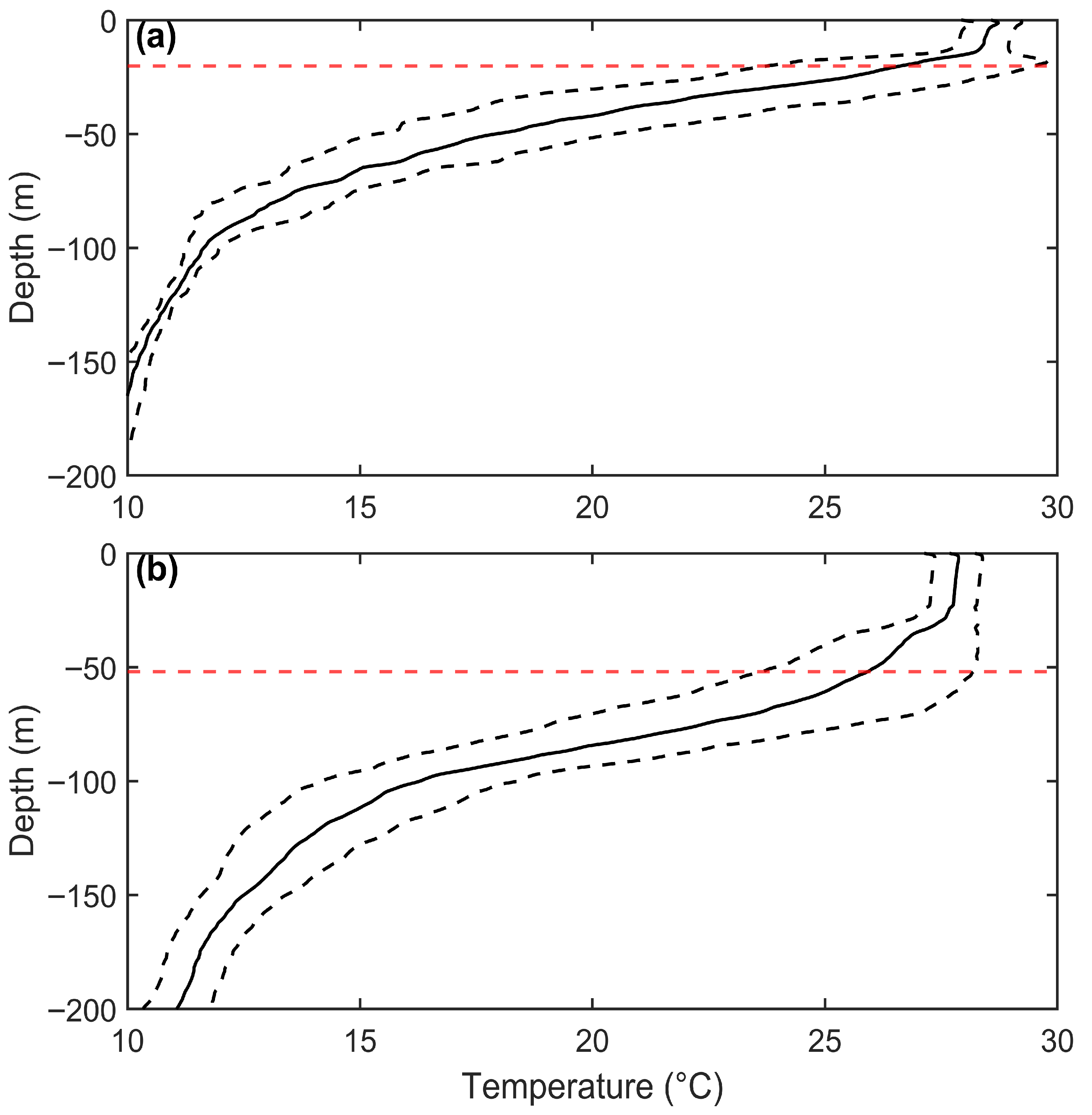
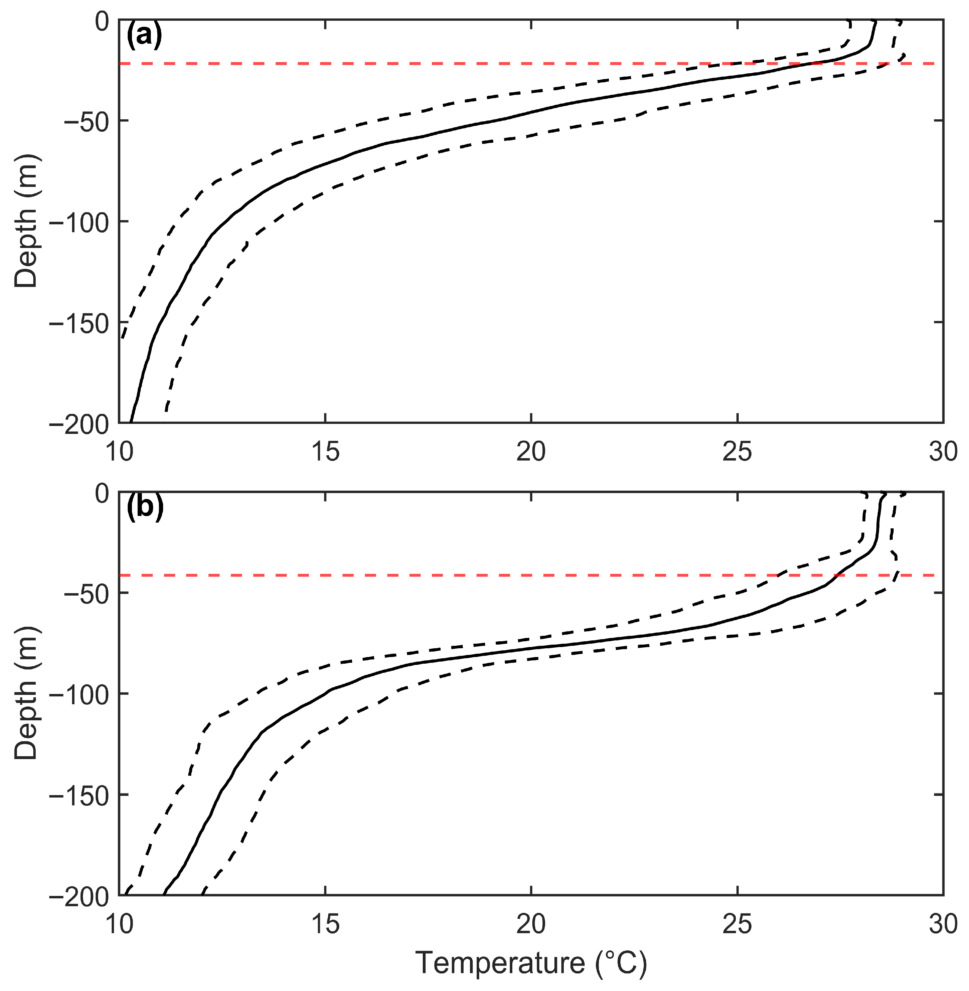
Average SST values in the northbound (southbound) path in inITCZ were 28.73 ± 0.50 °C (28.36 ± 0.62 °C) and 27.87 ± 0.51 °C (28.60 ± 0.46 °C) in outITCZ (

Table 8. Average $T_{sea}$ and SST values (with standard deviations) for the ITCZ and out of ITCZ regions during the northbound and southbound phases.

Zone	${\mathbf{T}}_{\mathbf{s}\mathbf{e}\mathbf{a}}$ (°C)	SST (°C)
	Northbound	Southbound
inITCZ	17.55 ± 6.40	17.88 ± 6.33
outITCZ	21.95 ± 5.95	21.83 ± 6.30

). Thus, no significant synoptic-scale changes can be observed for SST (Table A2). The ILD estimation method proposed by Kara et al. [45] appeared well aligned with the average temperature profiles (+standard deviation) for inITCZ and outITCZ (Figure 14 and Figure 15), although for both phases of the PBR18-3 campaign, it is possible to spot the oceanic barrier layers above the red line in Figure 14 and Figure 15. For outITCZ, the estimated ILD displayed higher variability, likely due to the spatial variability associated with the ED, dynamic processes influencing the upper ocean, and stronger surface wind patterns (speed and variability). These findings suggest the ED may not always be located directly beneath the ITCZ. Instead, its position might be influenced by vertical mixing, which in turn is strongly dependent on prevailing atmospheric conditions, like wind patterns.

4. Conclusions

The PBR18-3 campaign occurred between October and November in the austral spring of 2018, when the ITCZ was in its northernmost position, the southeasterly trade winds prevailed, and the retroflection of the NBC fed the NECC. Our main goal was to use meteorological and oceanographic observational data to describe the short-term atmospheric changes within the MABL and the consequent impacts on the ITCZ and the ED.

Because defining the ITCZ’s meridional boundaries can be complex and, sometimes, subjective, we used multiple variables to determine them between 6° N and 12° N. In the inITCZ region, the OLR and ${\mathrm{T}}_{\mathrm{a}\mathrm{i}\mathrm{r}}$ (${\mathrm{q}}_{\mathrm{z}}$) are significantly lower (higher) than in the outITCZ region. With the entry of northeast trades in the southbound path, the ITCZ intensified, along with lower (higher) OLR and ${\mathrm{T}}_{\mathrm{a}\mathrm{i}\mathrm{r}}$ (${\mathrm{q}}_{\mathrm{z}}$) values in the inITCZ. No significant SST changes were observed in the study period, as this is a region of minimal horizontal gradients.

In response to the synoptic-scale atmospheric changes, the ED exhibited a rapid response. During the northbound path, the ED was present as an asymmetric structure, with ILDs (~−14 m) around 11° N, whereas during the southbound route, the ED transitioned to a more homogenous region between 5° N and 10° N, with a mean ILD of −21.83 ± 5.23 m. Therefore, the ED is not directly below the ITCZ (here defined as in between 6° N and 12° N) at all times; rather, its position depends on wind patterns, upper-ocean dynamics, vertical mixing conditions, and the inherent inertia of the ocean. For the ED region, the ILD method showcased good results and appears to estimate an OML close to the MLD.

Both ORAS5 and WOA23 also exhibit warmer temperatures (~3–4 °C) near the bottom of the ILD and an overall colder water column (~−2 °C) when compared to observations. The NBUC, EUC, and NEUC cores are particularly colder in both datasets but were better represented by WOA23, likely due to current limitations in data assimilation and observational coverage that comprise ORAS5 [43,44]. Still, the oceanic variability observed in the XBT data is well captured by ORAS5 and WOA23, which represent the main water masses and associated features of the ITCZ and the ED.

The anomalies found during the study period may be associated with TIWs, which call for further investigation. However, part of these anomalies could also reflect temporal sampling mismatches between the synoptic-scale observational data and the monthly (hourly) oceanic (atmospheric) re-analysis/analysis data, potentially leading to an overestimation of the observed biases. This overestimation could impact model simulations, as accurate OML representation is essential for realistic ocean state modeling [56], and hurricane forecasting in the WTAO, given the role played by ocean heat content in the formation and intensification of tropical cyclones in the Atlantic Ocean’s main development region. Accurate representation of the oceanic heat content is therefore essential for timely responses and contingency planning [24,62,75,76].

This research contains inherent limitations, and as such, some of the results presented in this research should be interpreted carefully for a few reasons. First, all data used is inherently subject to operational and methodological uncertainties, including the possibility of human-induced errors, especially considering the aforementioned temporal mismatch between the analyzed data. Second, while many synoptic-scale studies focus on atmospheric equatorial wave activity and its role in modulating ITCZ-related cloudiness, this study has chosen to characterize ocean–atmosphere interactions and thus did not address atmospheric or oceanic (TIW) wave dynamics. Third, the in situ observations used here are limited to the 38° W meridian, as part of the PIRATA mooring array. However, we highlight that other regions of the TAO are also of significant interest and would benefit from similar in situ efforts to support multiscale ocean–atmosphere research. This includes enhanced monitoring, the expansion of in situ observations, and the integration of numerical modeling for robust analyses that are not feasible using observational data alone.

This study presents previously undocumented synoptic-scale variability of the WTAO ITCZ and its effects on the underlying ocean, based on XBT and radiosonde data. We recommend that future research explore ocean–atmosphere interactions across different temporal scales, integrate the use of coupled regional numerical models to simulate these processes, incorporate analyses of surface fluxes (including sensible and latent heat, momentum, and CO₂), and maybe explore the effects of different physical parametrizations in representing ITCZ–ED coupling. Such approaches may offer valuable insights, further advance the understanding of ITCZ dynamics, and fill gaps that this work could not address.

References

1. Foltz, G.R.; Grodsky, S.A.; Carton, J.A.; McPhaden, M.J. Seasonal Mixed Layer Heat Budget of the Tropical Atlantic Ocean. J. Geophys. Res. Ocean. 2003, 108, 3146. [Google Scholar] [CrossRef]
2. Foltz, G.R.; Eddebbar, Y.A.; Sprintall, J.; Capotondi, A.; Cravatte, S.; Brandt, P.; Sutton, A.J.; Morris, T.; Hermes, J.; McMahon, C.R.; et al. Toward an Integrated Pantropical Ocean Observing System. Front. Mar. Sci. 2025, 12, 1539183. [Google Scholar] [CrossRef]
3. Cabos, W.; de la Vara, A.; Koseki, S. Tropical Atlantic Variability: Observations and Modeling. Atmosphere 2019, 10, 502. [Google Scholar] [CrossRef]
4. Chen, S.-H.; Huang, C.-C.; Kuo, Y.-C.; Tseng, Y.-H.; Gu, Y.; Earl, K.; Chen, C.-Y.; Choi, Y.; Liou, K.-N. Impacts of Saharan Mineral Dust on Air-Sea Interaction over North Atlantic Ocean Using a Fully Coupled Regional Model. J. Geophys. Res. Atmos. 2021, 126, e2020JD033586. [Google Scholar] [CrossRef]
5. Xie, S.-P.; Carton, J.A. Tropical Atlantic Variability: Patterns, Mechanisms, and Impacts. Earth’s Clim. Ocean. -Atmos. Interact. Geophys. Monogr. 2004, 147, 121–142. [Google Scholar]
6. Lübbecke, J.F.; Richter, I.; Nnamchi, H.C. Dynamics of Tropical Atlantic Variability. In CLIVAR Exchanges: Tropical Atlantic Ocean Observing System (TAOS); ICPO: Qingdao, China, 2022; Volume 82, pp. 9–14. [Google Scholar] [CrossRef]
7. Moura, A.D.; Shukla, J. On the Dynamics of Droughts in Northeast Brazil: Observations, Theory and Numerical Experiments with a General Circulation Model. J. Atmos. Sci. 1981, 38, 2653–2675. [Google Scholar] [CrossRef]
8. de Carvalho, M.Â.V.; Oyama, M.D. Variabilidade Da Largura e Intensidade Da Zona de Convergência Intertropical Atlântica: Aspectos Observacionais. Rev. Bras. Meteorol. 2013, 28, 305–316. [Google Scholar] [CrossRef]
9. Speich, S.; Araujo, M.; Balmaseda, M.; Bourlès, B.; Foltz, G.; McPhaden, M.J.; Rodrigues, R.R. An Introduction to the Tropical Atlantic Ocean Observing System: Past and Present. In CLIVAR Exchanges: Tropical Atlantic Ocean Observing System (TAOS); ICPO: Qingdao, China, 2022; Volume 82, pp. 3–8. [Google Scholar] [CrossRef]
10. Doi, T.; Vecchi, G.A.; Rosati, A.J.; Delworth, T.L. Biases in the Atlantic ITCZ in Seasonal–Interannual Variations for a Coarse-and a High-Resolution Coupled Climate Model. J. Clim. 2012, 25, 5494–5511. [Google Scholar] [CrossRef]
11. Richter, I.; Xie, S.-P.; Behera, S.K.; Doi, T.; Masumoto, Y. Equatorial Atlantic Variability and Its Relation to Mean State Biases in CMIP5. Clim. Dyn. 2014, 42, 171–188. [Google Scholar] [CrossRef]
12. Siongco, A.C.; Hohenegger, C.; Stevens, B. The Atlantic ITCZ Bias in CMIP5 Models. Clim. Dyn. 2015, 45, 1169–1180. [Google Scholar] [CrossRef]
13. Laurido, A.L.C.; Solórsano, Á.G.M.; Chourio, X.; Mosquera, C.A.T.; Latandret, S. Seasonal-To-Interannual Variability of Sea-Surface Temperatures in The Inter-Americas Seas: Pattern-Dependent Biases in The Regional Ocean Modeling System. ACI Av. Cienc. Ing. 2021, 13, 20. [Google Scholar] [CrossRef]
14. Lee, J.; Kang, S.M.; Kim, H.; Xiang, B. Disentangling the Effect of Regional SST Bias on the Double-ITCZ Problem. Clim. Dyn. 2022, 58, 3441–3453. [Google Scholar] [CrossRef]
15. Luo, F.; Ying, J.; Liu, T.; Chen, D. Origins of Southern Ocean Warm Sea Surface Temperature Bias in CMIP6 Models. npj Clim. Atmos. Sci. 2023, 6, 127. [Google Scholar] [CrossRef]
16. Dong, E.; Song, F.; Wu, L.; Dong, L.; Wang, S.; Liu, F.; Wang, H. The Process-Oriented Understanding on the Reduced Double-ITCZ Bias in the High-Resolution CESM1. Geophys. Res. Lett. 2025, 52, e2024GL112087. [Google Scholar] [CrossRef]
17. Diedhiou, A.; Janicot, S.; Viltard, A.; De Felice, P.; Laurent, H. Easterly Wave Regimes and Associated Convection over West Africa and Tropical Atlantic: Results from the NCEP/NCAR and ECMWF Reanalyses. Clim. Dyn. 1999, 15, 795–822. [Google Scholar] [CrossRef]
18. Serra, Y.L.; Houze, R.A., Jr. Observations of Variability on Synoptic Timescales in the East Pacific ITCZ. J. Atmos. Sci. 2002, 59, 1723–1743. [Google Scholar] [CrossRef]
19. Wang, C.; Magnusdottir, G. The ITCZ in the Central and Eastern Pacific on Synoptic Time Scales. Mon. Weather. Rev. 2006, 134, 1405–1421. [Google Scholar] [CrossRef]
20. Wang, H.; Fu, R. The Influence of Amazon Rainfall on the Atlantic ITCZ through Convectively Coupled Kelvin Waves. J. Clim. 2007, 20, 1188–1201. [Google Scholar] [CrossRef]
21. Nogueira, N.C.d.O.; Machado, P.H.G.; Reboita, M.S.; Reis, A.L. Assessment of the Intertropical Convergence Zone over the Atlantic Ocean through an Algorithm Based on Precipitation. J. Atmos. Sci. Res. 2024, 7, 59–73. [Google Scholar] [CrossRef]
22. Goswami, B.N.; Shukla, J.; Schneider, E.; Sud, Y. Study of the Dynamics of the Intertropical Convergence Zone with a Symmetric Version of the GLAS Climate Model. J. Atmos. Sci. 1984, 41, 5–19. [Google Scholar] [CrossRef]
23. Bourlès, B.; Araujo, M.; McPhaden, M.J.; Brandt, P.; Foltz, G.R.; Lumpkin, R.; Giordani, H.; Hernandez, F.; Lefèvre, N.; Nobre, P.; et al. PIRATA: A Sustained Observing System for Tropical Atlantic Climate Research and Forecasting. Earth Space Sci. 2019, 6, 577–616. [Google Scholar] [CrossRef]
24. Foltz, G.R.; Brandt, P.; Richter, I.; Rodríguez-Fonseca, B.; Hernandez, F.; Dengler, M.; Rodrigues, R.R.; Schmidt, J.O.; Yu, L.; Lefevre, N.; et al. The Tropical Atlantic Observing System. Front. Mar. Sci. 2019, 6, 206. [Google Scholar] [CrossRef]
25. Foltz, G.R.; Grodsky, S.A.; Carton, J.A.; McPhaden, M.J. Seasonal Salt Budget of the Northwestern Tropical Atlantic Ocean along 38 W. J. Geophys. Res. Ocean. 2004, 109, C03052. [Google Scholar] [CrossRef]
26. Foltz, G.R.; Hummels, R.; Dengler, M.; Perez, R.C.; Araujo, M. Vertical Turbulent Cooling of the Mixed Layer in the Atlantic ITCZ and Trade Wind Regions. J. Geophys. Res. Ocean. 2020, 125, e2019JC015529. [Google Scholar] [CrossRef]
27. Talley, L.D. Descriptive Physical Oceanography: An Introduction; Academic Press: Cambridge, MA, USA, 2011. [Google Scholar]
28. Weingartner, T.J.; Weisberg, R.H. On the Annual Cycle of Equatorial Upwelling in the Central Atlantic Ocean. J. Phys. Oceanogr. 1991, 21, 68–82. [Google Scholar] [CrossRef]
29. Faria, A.L.S.; de Freitas, R.A.P.; de Souza, R.B.; Wallner-Kersanach, M.; Evangelista, H.; Moura, R.; Contreira-Pereira, L.; Mirlean, N.; Seus-Arrache, E.R.; da Costa Machado, E. The Role of the Intertropical Convergence Zone on the Aerosol Transport Pathways From Africa Towards the Western Tropical Atlantic Ocean. Int. J. Climatol. 2025, 45, e8910. [Google Scholar] [CrossRef]
30. Musetti de Assis, C.A.; Pinho, L.Q.; Fernandes, A.M.; Araujo, M.; Cotrim da Cunha, L. Reconstruction of the Marine Carbonate System at the Western Tropical Atlantic: Trends and Variabilities from 20 Years of the PIRATA Program. Front. Mar. Sci. 2024, 11, 1286960. [Google Scholar] [CrossRef]
31. Pérez, V.; Fernández, E.; Marañón, E.; Serret, P.; Varela, R.; Bode, A.; Varela, M.; Varela, M.M.; Morán, X.A.G.; Woodward, E.M.S.; et al. Latitudinal Distribution of Microbial Plankton Abundance, Production, and Respiration in the Equatorial Atlantic in Autumn 2000. Deep. Sea Res. Part I Oceanogr. Res. Pap. 2005, 52, 861–880. [Google Scholar] [CrossRef]
32. Farias, G.B.; Molinero, J.-C.; Carré, C.; Bertrand, A.; Bec, B.; de Castro Melo, P.A.M. Uncoupled Changes in Phytoplankton Biomass and Size Structure in the Western Tropical Atlantic. J. Mar. Syst. 2022, 227, 103696. [Google Scholar] [CrossRef]
33. Menezes, M.; Junger, P.C.; Kavagutti, V.S.; Wanderley, B.; Cabral, A.d.S.; Paranhos, R.; Unrein, F.; Amado, A.M.; Sarmento, H. Temporal Patterns of Picoplankton Abundance and Metabolism on the Western Coast of the Equatorial Atlantic Ocean. Ocean. Coast. Res. 2023, 71, e23019. [Google Scholar] [CrossRef]
34. Ogundare, M.O.; Adekunbi, F.O. Seasonal and Interannual Variability in Carbon Dioxide Fluxes in the Tropical Atlantic. Open Access Libr. J. 2024, 11, e12718. [Google Scholar] [CrossRef]
35. Johns, W.E.; Lee, T.N.; Schott, F.A.; Zantopp, R.J.; Evans, R.H. The North Brazil Current Retroflection: Seasonal Structure and Eddy Variability. J. Geophys. Res. Ocean. 1990, 95, 22103–22120. [Google Scholar] [CrossRef]
36. Richardson, P.; Hufford, G.; Limeburner, R.; Brown, W. North Brazil Current Retroflection Eddies. J. Geophys. Res. Ocean. 1994, 99, 5081–5093. [Google Scholar] [CrossRef]
37. Fernández, P.; Speich, S.; Bellenger, H.; Lange Vega, D.; Karstensen, J.; Zhang, D.; Rocha, C.B. On the Mechanisms Driving Latent Heat Flux Variations in the Northwest Tropical Atlantic. J. Geophys. Res. Ocean. 2024, 129, e2023JC020658. [Google Scholar] [CrossRef]
38. Souza, R.; Pezzi, L.; Swart, S.; Oliveira, F.; Santini, M. Air-Sea Interactions over Eddies in the Brazil-Malvinas Confluence. Remote Sens. 2021, 13, 1335. [Google Scholar] [CrossRef]
39. Hersbach, H.; Bell, B.; Berrisford, P.; Hirahara, S.; Horányi, A.; Muñoz-Sabater, J.; Nicolas, J.; Peubey, C.; Radu, R.; Schepers, D.; et al. The ERA5 Global Reanalysis. Q. J. R. Meteorol. Soc. 2020, 146, 1999–2049. [Google Scholar] [CrossRef]
40. Hummels, R.; Brandt, P.; Dengler, M.; Fischer, J.; Araujo, M.; Veleda, D.; Durgadoo, J.V. Interannual to Decadal Changes in the Western Boundary Circulation in the Atlantic at 11°S. Geophys. Res. Lett. 2015, 42, 7615–7622. [Google Scholar] [CrossRef]
41. Brandt, P.; Claus, M.; Greatbatch, R.J.; Kopte, R.; Toole, J.M.; Johns, W.E.; Böning, C.W. Annual and Semiannual Cycle of Equatorial Atlantic Circulation Associated with Basin-Mode Resonance. J. Phys. Oceanogr. 2016, 46, 3011–3029. [Google Scholar] [CrossRef]
42. Zuo, H.; Alonso-Balmaseda, M.; Mogensen, K.; Tietsche, S. OCEAN5: The ECMWF Ocean Reanalysis System and Its Real-Time Analysis Component; ECMWF Technical Memoranda; ECMWF: Reading, UK, 2018. [Google Scholar]
43. Zuo, H.; Balmaseda, M.A.; Tietsche, S.; Mogensen, K.; Mayer, M. The ECMWF Operational Ensemble Reanalysis–Analysis System for Ocean and Sea Ice: A Description of the System and Assessment. Ocean. Sci. 2019, 15, 779–808. [Google Scholar] [CrossRef]
44. Liu, H.; Wei, Z.; Richter, I.; Nie, X.; Li, C. Influence of Salinity and Temperature Gradients on the Variability of the North Brazil Undercurrent. Front. Mar. Sci. 2021, 8, 744833. [Google Scholar] [CrossRef]
45. Kara, A.B.; Rochford, P.A.; Hurlburt, H.E. An Optimal Definition for Ocean Mixed Layer Depth. J. Geophys. Res. Ocean. 2000, 105, 16803–16821. [Google Scholar] [CrossRef]
46. de Boyer Montégut, C.; Madec, G.; Fischer, A.S.; Lazar, A.; Iudicone, D. Mixed Layer Depth over the Global Ocean: An Examination of Profile Data and a Profile-Based Climatology. J. Geophys. Res. Ocean. 2004, 109, C12003. [Google Scholar] [CrossRef]
47. Holte, J.; Talley, L. A New Algorithm for Finding Mixed Layer Depths with Applications to Argo Data and Subantarctic Mode Water Formation. J. Atmos. Ocean. Technol. 2009, 26, 1920–1939. [Google Scholar] [CrossRef]
48. Saha, A.; Serra, N.; Stammer, D. Growth and Decay of Northwestern Tropical Atlantic Barrier Layers. J. Geophys. Res. Ocean. 2021, 126, e2020JC016956. [Google Scholar] [CrossRef]
49. Ma, X.; Liu, H.; Wang, X. Interannual Variability of Barrier Layer in the Tropical Atlantic and Its Relationship with the Tropical Atlantic Modes. J. Phys. Oceanogr. 2023, 53, 573–594. [Google Scholar] [CrossRef]
50. Lukas, R.; Lindstrom, E. The Mixed Layer of the Western Equatorial Pacific Ocean. J. Geophys. Res. Ocean. 1991, 96, 3343–3357. [Google Scholar] [CrossRef]
51. Rabelo, L.B.; de Souza, R.B.; Mata, M.M.; Santini, M.F. Estrutura Termal Em Alta Resolução Das Águas Da Frente Polar Na Região Da Passagem de Drake Durante as Operações Antárticas XXII e XXIII (Verão Austral de 2003 e 2004). Atlântica 2012, 34, 189–201. [Google Scholar] [CrossRef]
52. Dohan, K. Ocean Surface Current Analyses Real-Time (OSCAR) Surface Currents—Interim 0.25 Degree (Version 2.0); NASA Physical Oceanography Distributed Active Archive Center: Pasadena, CA, USA, 2021. [Google Scholar]
53. Pezzi, L.P.; de Souza, R.B.; Quadro, M.F. Uma Revisão Dos Processos de Interação Oceano-Atmosfera Em Regiões de Intenso Gradiente Termal Do Oceano Atlântico Sul Baseada Em Dados Observacionais. Rev. Bras. Meteorol. 2016, 31, 428–453. [Google Scholar] [CrossRef]
54. de Freitas, R.A.P.; de Souza, R.B.; do Nascimento Reis, R.A.; de Mendonça, L.F.F.; da Silva Lindemann, D. Satellite and in Situ Measurements of Water Vapour in the Brazil-Malvinas Confluence Region. Int. J. Climatol. 2024, 44, 4286–4305. [Google Scholar] [CrossRef]
55. Ho, S.-P.; Gu, G.; Zhou, X. The Planetary Boundary Layer Height Climatology over Oceans Using COSMIC-2 and Spire GNSS RO Bending Angles from 2019 to 2023: Comparisons to CALIOP, ERA-5, MERRA2, and CFS Reanalysis. IEEE Trans. Geosci. Remote Sens. 2024, 62, 5803314. [Google Scholar] [CrossRef]
56. Karmakar, A.; Parekh, A.; Chowdary, J.; Gnanaseelan, C. Inter Comparison of Tropical Indian Ocean Features in Different Ocean Reanalysis Products. Clim. Dyn. 2018, 51, 119–141. [Google Scholar] [CrossRef]
57. Goes, M.; Molinari, R.; da Silveira, I.; Wainer, I. Retroflections of the North Brazil Current during February 2002. Deep. Sea Res. Part I Oceanogr. Res. Pap. 2005, 52, 647–667. [Google Scholar] [CrossRef]
58. Locarnini, R.A.; Mishonov, A.V.; Baranova, O.K.; Reagan, J.R.; Boyer, T.P.; Seidov, D.; Wang, Z.; Garcia, H.E.; Bouchard, C.; Cross, S.L.; et al. World Ocean Atlas 2023, Volume 1: Temperature. NOAA Repos. 2024, 1. [Google Scholar] [CrossRef]
59. Stramma, L.; Schott, F. The Mean Flow Field of the Tropical Atlantic Ocean. Deep. Sea Res. Part II Top. Stud. Oceanogr. 1999, 46, 279–303. [Google Scholar] [CrossRef]
60. Zhang, D.; Msadek, R.; McPhaden, M.J.; Delworth, T. Multidecadal Variability of the North Brazil Current and Its Connection to the Atlantic Meridional Overturning Circulation. J. Geophys. Res. Ocean. 2011, 116, C04012. [Google Scholar] [CrossRef]
61. Dossa, A.N.; Silva, A.C.; Chaigneau, A.; Eldin, G.; Araujo, M.; Bertrand, A. Near-Surface Western Boundary Circulation off Northeast Brazil. Prog. Oceanogr. 2021, 190, 102475. [Google Scholar] [CrossRef]
62. Mainelli, M.; DeMaria, M.; Shay, L.K.; Goni, G. Application of Oceanic Heat Content Estimation to Operational Forecasting of Recent Atlantic Category 5 Hurricanes. Weather. Forecast. 2008, 23, 3–16. [Google Scholar] [CrossRef]
63. Saunders, M.; Klotzbach, P.; Lea, A.; Schreck, C.; Bell, M. Quantifying the Probability and Causes of the Surprisingly Active 2018 North Atlantic Hurricane Season. Earth Space Sci. 2020, 7, e2019EA000852. [Google Scholar] [CrossRef]
64. Han, Y.; Zhai, W.; Mozumder, P.; van Westen, C.; Chen, C. Modeling Evacuation Activities amid Compound Hazards: Insights from Hurricane Irma in Southeast Florida. Travel Behav. Soc. 2025, 38, 100933. [Google Scholar] [CrossRef]
65. dos Reis, B.L.R.; Parise, C.K.; Correia, G.S.; de Lima, L.G.; Perotto, H.; Bose, N.d.A.; de Mendonça, L.F.F. The Bimodal Regime of Ocean Waves and Winds over the Continental Shelf of Maranhão. Reg. Stud. Mar. Sci. 2024, 77, 103629. [Google Scholar] [CrossRef]
66. Harris, E.A.; Marsh, R.; Grist, J.P. Tracing Oceanic Sources of Heat Content Available for Atlantic Hurricanes. J. Geophys. Res. Ocean. 2023, 128, e2022JC019407. [Google Scholar] [CrossRef]
67. Costa da Silva, A.; Chaigneau, A.; Dossa, A.N.; Eldin, G.; Araujo, M.; Bertrand, A. Surface Circulation and Vertical Structure of Upper Ocean Variability around Fernando de Noronha Archipelago and Rocas Atoll during Spring 2015 and Fall 2017. Front. Mar. Sci. 2021, 8, 598101. [Google Scholar] [CrossRef]
68. Richter, I.; Xie, S.-P.; Morioka, Y.; Doi, T.; Taguchi, B.; Behera, S. Phase Locking of Equatorial Atlantic Variability through the Seasonal Migration of the ITCZ. Clim. Dyn. 2017, 48, 3615–3629. [Google Scholar] [CrossRef]
69. von Schuckmann, K.; Brandt, P.; Eden, C. Generation of Tropical Instability Waves in the Atlantic Ocean. J. Geophys. Res. Ocean. 2008, 113, C08034. [Google Scholar] [CrossRef]
70. Liu, C.; Köhl, A.; Liu, Z.; Wang, F.; Stammer, D. Deep-Reaching Thermocline Mixing in the Equatorial Pacific Cold Tongue. Nat. Commun. 2016, 7, 11576. [Google Scholar] [CrossRef] [PubMed]
71. Fang, L.; Ma, K.; Liu, C.; Wang, X.; Wang, F. Ocean Mixing Induced by Three-Dimensional Structure of Equatorial Mode Tropical Instability Waves in the Pacific Ocean. Front. Mar. Sci. 2023, 10, 1228897. [Google Scholar] [CrossRef]
72. Gaube, P.; McGillicuddy, D.J., Jr.; Moulin, A.J. Mesoscale Eddies Modulate Mixed Layer Depth Globally. Geophys. Res. Lett. 2019, 46, 1505–1512. [Google Scholar] [CrossRef]
73. Vilela, I.; Araujo, M.; Tyaquiçã, P.; Veleda, D. Empirical Orthogonal Function Analysis of Satellite-Derived Currents in the Tropical Atlantic. Trop. Oceanogr. 2018, 46, 1–24. [Google Scholar]
74. Utida, G.; Cruz, F.W.; Etourneau, J.; Bouloubassi, I.; Schefuß, E.; Vuille, M.; Novello, V.F.; Prado, L.F.; Sifeddine, A.; Klein, V.; et al. Tropical South Atlantic Influence on Northeastern Brazil Precipitation and ITCZ Displacement during the Past 2300 Years. Sci. Rep. 2019, 9, 1698. [Google Scholar] [CrossRef]
75. Hallam, S.; Marsh, R.; Josey, S.A.; Hyder, P.; Moat, B.; Hirschi, J.J.-M. Ocean Precursors to the Extreme Atlantic 2017 Hurricane Season. Nat. Commun. 2019, 10, 896. [Google Scholar] [CrossRef] [PubMed]
76. Trenberth, K.E.; Cheng, L.; Jacobs, P.; Zhang, Y.; Fasullo, J. Hurricane Harvey Links to Ocean Heat Content and Climate Change Adaptation. Earth’s Future 2018, 6, 730–744. [Google Scholar] [CrossRef]
Figure 1. Averaged SST field for the study period along the 38° W transect during the PBR18-3 campaign, denoted by the black line. The radiosonde (white circles) and XBT (black circles) markers are the launching positions during both the northbound (n) and southbound (s) paths. The dashed grey lines separate the inside and outside of the ITCZ, as defined in Section 3.1.
Atmosphere 17 00101 g001
Figure 2. Meridional sections of the atmospheric mixing ratio ( q z ) and the meridional component of the wind in the atmosphere up to 2000 m during the northbound (a) and southbound (b) paths of the ship’s route in the PBR18-3 campaign. The difference in q z between the two paths of the ship’s route can be seen in (c).
Atmosphere 17 00101 g002
Figure 3. Map of the mean OLR in the WTAO during both northbound (a) and southbound (b) paths of the ship’s route in the PBR18-3 campaign. The difference in OLR between the two paths of the ship’s route (black line) can be seen in (c). The radiosonde (black circles) launching positions taken during the PBR18-3 campaign are also shown.
Atmosphere 17 00101 g003
Figure 4. Vertical water temperature transects at the 38° W meridian based on (a) XBT data obtained during the northbound path of the PBR18-3 campaign, (b) ORAS5 data for October 2018, (c) ORAS5 October climatology, and (d) WOA23 October climatology. The white triangles represent the launched XBTs, while the estimated ILD along the transects is shown as a yellow line for each dataset.
Atmosphere 17 00101 g004
Figure 5. Vertical water temperature transects at the 38° W meridian based on (a) XBT data obtained during the southbound path of the PBR18-3 campaign, (b) ORAS5 data for November 2018, (c) ORAS5 November climatology, and (d) WOA23 November climatology. The white triangles represent the launched XBTs, while the estimated ILD along the transects is shown as a yellow line for each dataset.
Atmosphere 17 00101 g005
Figure 6. Water temperature difference (biases) transects between observational (XBT) and other datasets obtained for the northbound path of the PRB18-3 campaign: (a) ORAS5 October 2018 average minus XBT; (b) ORAS5 October climatology minus XBT, and (c) WOA23 October climatology minus XBT. The ILD estimated from the XBT data is shown by the black line, while the ILD (MLD) estimated from each other dataset is shown by the red (green) line.
Atmosphere 17 00101 g006
Figure 7. Water temperature difference (biases) transects between observational (XBT) and other datasets obtained for the southbound path of the PBR18-3 campaign: (a) ORAS5 November 2018 average minus XBT; (b) ORAS5 November climatology minus XBT, and (c) WOA23 November climatology minus XBT. The ILD estimated from the XBT data is shown by the black line, while the ILD (MLD) estimated from each other dataset is shown by the red (green) line.
Atmosphere 17 00101 g007
Figure 8. Linear correlations between XBT and (a) ORAS5 October 2018; (b) ORAS5 October climatology; and (c) WOA23 October climatology for the northbound path of the PBR18-3 campaign.
Atmosphere 17 00101 g008
Figure 9. Linear correlations between XBT and (a) ORAS5 November 2018; (b) ORAS5 November climatology; and (c) WOA23 November climatology for the southbound path of the PBR18-3 campaign.
Atmosphere 17 00101 g009
Figure 10. θ-S diagrams of four latitudinal bands: 5° S–0° (a), 0°–5° N (b), 5° N–10° N (c), and 10° N–15° N (d), based on the ORAS5 October (dark blue) and November (dark red) climatologies. The dashed squares represent the θ and S ranges of each water mass: TSW, SUW and SACW.
Atmosphere 17 00101 g010
Figure 11. θ-S diagrams of four latitudinal bands: 5° S–0° (a), 0°–5° N (b), 5° N–10° N (c), and 10° N–15° N (d), based on the WOA23 October (dark blue) and November (dark red) climatologies. The dashed squares represent the θ and S ranges of each water mass: TSW, SUW and SACW.
Atmosphere 17 00101 g011
Figure 12. Average ocean surface currents vectors (black arrows) for the northbound (a) and southbound (b) phases of the PBR18-3 campaign, based on data from Project OSCAR. The path sailed by the R/V Vital de Oliveira is represented by the dashed golden line.
Atmosphere 17 00101 g012
Figure 13. Vertical water and air temperature transects at the 38° W meridian based on XBT and radiosonde data obtained during the northbound (a) and southbound (b) phases of the PBR18-3 campaign. The synoptic-scale difference between the southbound and northbound phases is also shown in (c), along with the white triangles representing the launched XBTs and the estimated ILD for each phase being represented by the black (northbound) and red lines (southbound).
Atmosphere 17 00101 g013
Figure 14. Averaged XBT temperature (solid black lines) profiles (±standard deviation – dashed black lines) for inITCZ (a) and outITCZ (b) for the northbound phase. The red dashed line illustrates the average estimated ILD.
Atmosphere 17 00101 g014
Figure 15. Averaged XBT temperature (solid black lines) profiles (±standard deviation – dashed black lines) for inITCZ (a) and outITCZ (b) for the southbound phase. The red dashed line illustrates the average estimated ILD.
Atmosphere 17 00101 g015