Article

Vegetation Dynamics and Atmospheric Glyoxal in Houston, Texas (2018–2022)

by
Salma Bibi
1,2,* and
Bernhard Rappenglück
1,2
1
Department of Earth and Atmospheric Sciences, University of Houston, Houston, TX 77204, USA
2
Institute for Climate and Atmospheric Science, University of Houston, Houston, TX 77204, USA
*
Author to whom correspondence should be addressed.
Atmosphere 2026, 17(1), 100; https://doi.org/10.3390/atmos17010100
Submission received: 20 November 2025 / Revised: 9 January 2026 / Accepted: 15 January 2026 / Published: 18 January 2026
(This article belongs to the Section Biosphere/Hydrosphere/Land–Atmosphere Interactions)

Abstract

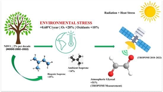
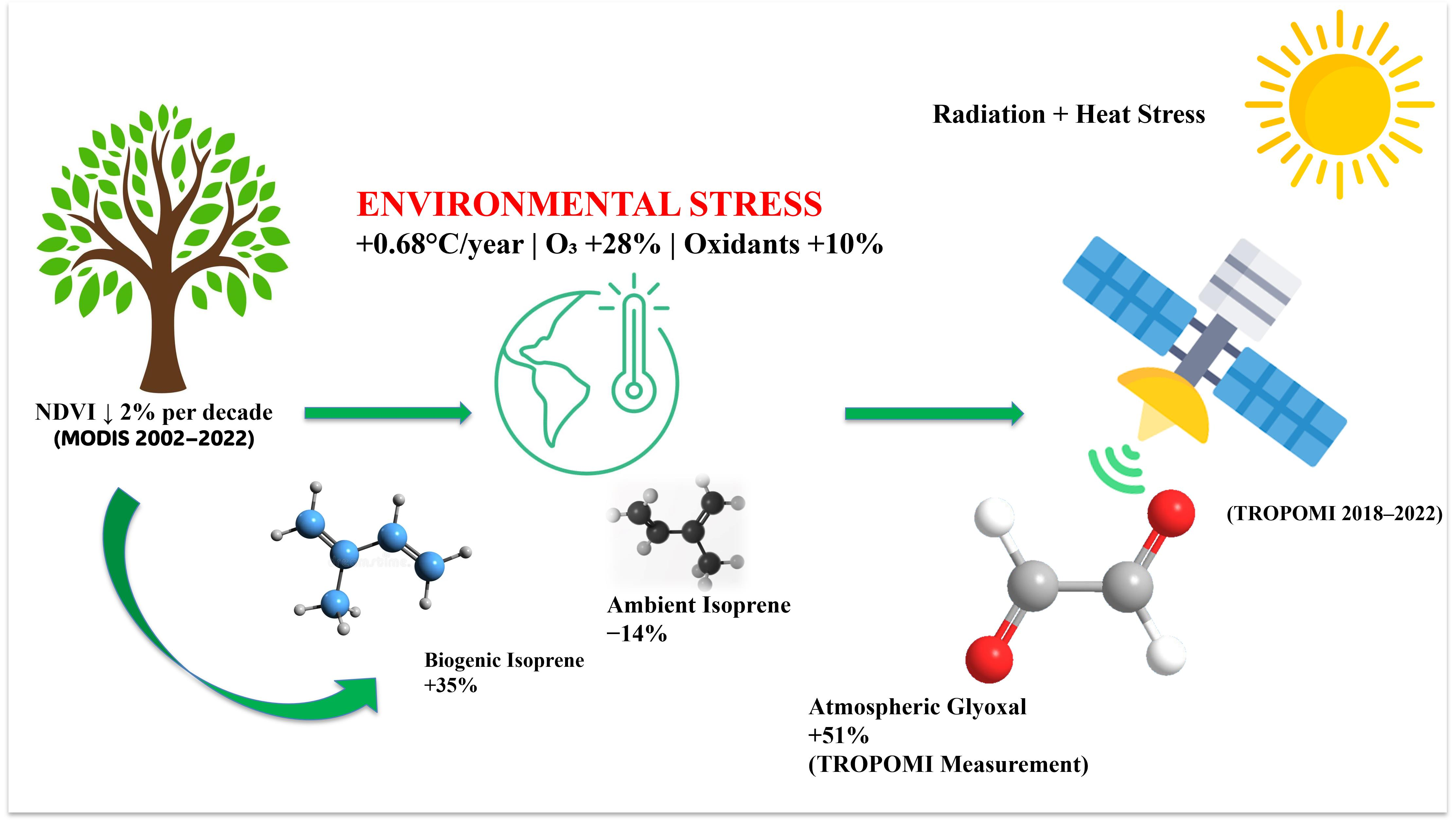
Twenty years of MODIS satellite data (2002–2022), TROPOMI glyoxal observations (2018–2022), and ground-based isoprene measurements were used to examine vegetation greenness (NDVI) and atmospheric glyoxal over Houston, Texas. Biogenically produced glyoxal grew by 51% between 2018 and 2022, despite a 2% per decade decrease in summer vegetation greenness and continued urbanization. Ambient mixing ratios of isoprene, the main biogenic glyoxal precursor, paradoxically dropped by 14% within the same time frame. Temperature (+0.68 °C/year), ozone (+28%), and photochemical oxidants all significantly increased over this time, according to analysis of concurrent environmental data. The results indicate that higher temperature-driven isoprene emissions (+35%) and accelerated photochemical oxidation (+10%) overcame the declining vegetation signal, resulting in net increases in atmospheric glyoxal. This suggests that Houston’s remaining flora is experiencing temperature-driven changes in biogenic volatile organic compound (VOC) emissions per unit area, even while its greenness has reduced.

Graphical Abstract

1. Introduction

Vegetation dynamics are essential for regulating ecosystem functioning, carbon sequestration, and climate–vegetation feedback [1]. Biogenic VOCs (BVOCs) are volatile organic compounds (VOCs) that are generated by secondary metabolic pathways in a variety of plant tissues, including leaves, flowers, fruits, and roots [2]. Both biogenic VOCs from vegetation and anthropogenic VOCs from human activities undergo atmospheric oxidation by the hydroxyl radical (OH) to form glyoxal (CHOCHO). The dominant biogenic VOC, isoprene (C5H8), produces glyoxal through a multi-step process initiated by OH, followed by oxygen addition to form peroxy radicals. These peroxy radicals subsequently react with nitrogen oxides (NOx) to create intermediates such methacrolein (MACR) and methyl vinyl ketone (MVK), which are then further oxidized by glycolaldehyde to form glyoxal with a 6.2% molar yield [3]. Aromatic hydrocarbons, mainly benzene, toluene, and p-xylene, as well as acetylene, are key anthropogenic precursors of glyoxal [4,5]. Their only atmospheric chemical removal process is OH-initiated oxidation in which OH radicals add to the aromatic ring, forming aromatic–OH complexes that react with atmospheric oxygen to produce bicycloalkyl radicals. After that, these intermediates undergo ring cleavage, producing glyoxal at approximately 35% ± 10% for benzene and approximately 5% higher for toluene and p-xylene [4]. Although these aromatics produce more glyoxal than isoprene, isoprene nevertheless has the highest emissions worldwide. Isoprene, emitted mainly by deciduous broadleaf species, is the most abundant BVOC globally (contributing about 50% of total BVOC emissions) and is the primary precursor of formaldehyde (HCHO) and glyoxal over vegetated areas [6,7]
Isoprene has a significant impact on atmospheric chemistry [8], including urban air quality in the presence of elevated NOx levels [9,10]. It is estimated that BVOC emissions from Beijing’s urban green spaces could contribute about 30% to ambient summer O3 under high-NOx conditions [11]., while another study discovered contributions of up to 4.74 ppbv to near-surface O3 in polluted urban areas of the Pearl River Delta, China [12].
Isoprene and glyoxal’s temporal association help differentiate between biogenic and anthropogenic glyoxal sources and sheds light on the chemistry of biogenic VOC oxidation. Glyoxal monitoring using satellite remote sensing provides information about the chemistry of VOC oxidation and how it contributes to the production of ozone (O3) and secondary organic aerosols (SOA) [13].
Empirical emission methodologies are frequently used to estimate biogenic emissions [14]. It considers vegetation type, leaf area density, short-term environmental correction variables that adjust emissions based on light intensity and temperature, and long-term correction factors that consider vegetation greenness, leaf age, and seasonal phenology. Temperature is the main factor affecting BVOC emissions from plants; rising temperatures often result in exponential increases in emission rates due to enzymatic activity and volatilization processes [15]. The Normalized Difference Vegetation Index (NDVI), which measures vegetation greenness, leaf area index, and photosynthetic capacity as an indicator of emission potential and is based on red and near-infrared reflectance data gathered by satellite sensors, is a widely used proxy for assessing long-term activity [16].
The urban area of Houston, Texas is located about 30° N and has a subtropical climate with hot humid summers and mostly mild winters. The combination of anthropogenic emissions released from large industrial aeras, including petrochemical sources along the Ship Channel and extensive urban activity [17,18,19,20], and high BVOC emission from subtropical vegetation during the warm growing season is especially important in metropolitan areas like Houston, Texas [21]. A recent analysis of a long-term trend analysis of VOC data in mostly maritime air masses in the Houston area found a statistically significant increasing trend of 0.45 ppbC year−1 from 2004 to 2023 [22]. They also discovered that isoprene accounts for 80–90% of the summer Propylene-Equivalent (Propy-Equiv) concentration. The increase was mostly linked to rising temperatures (1.58 ± 0.14 °C), which resulted in an estimated 20 ± 1.6% increase in isoprene emissions.
Following up on these long-term results, the purpose of this study is to investigate the relationship between atmospheric glyoxal production and vegetation dynamics in the Houston area. NDVI measurements are used as a vegetation activity indicator (2002–2022) to assess changes in greenness during the preceding 20 years. In order to identify the temporal and spatial emission patterns, tropospheric glyoxal column densities from TROPOMI (2018–2022) are examined concurrently.
This study integrated ground-based isoprene measurements with TROPOMI glyoxal vertical column densities during the growing season (May–October 2018–2022) to quantify biogenic contributions to atmospheric glyoxal in Houston. The analysis assesses the correlation between atmospheric glyoxal and vegetation greenness (NDVI), measures the temporal coupling between isoprene and glyoxal, and uses seasonal baselines to separate biogenic from anthropogenic glyoxal sources. The observed isoprene–glyoxal decoupling shows how oxidant levels and temperature affect the effectiveness of biogenic VOC oxidation. This is the first multi-year satellite–ground evaluation of biogenic glyoxal dynamics in Houston, showing how environmental conditions modify the chemical interaction between plant and the atmosphere in subtropical metropolitan settings

2. Study Area

The Greater Houston metropolitan area, located in the southeast Texas, is home to 7.8 million people and covers an area of about 26,000 km2, making it the fifth most populous metropolitan area in the US [23]. The area is home to significant economic hubs, including the Port of Houston [24]. As a major petrochemical and industrial hub surrounded by vegetation, emissions from both biogenic (vegetation) and anthropogenic (industrial, vehicle) sources are present in the area [17,18,19,20]. The region’s long growth season, which is fueled by its subtropical, humid climate with hot, muggy summers and mild winters, produces significant biogenic emissions. Significant seasonal variability in volatile organic compounds (VOCs), including isoprene, is confirmed by atmospheric observations in the Houston area [20,22].
Significant urbanization occurred in Harris County, where large portions of the Houston area is located; between 2001 and 2019, urban land cover grew by 15.2%, while forest cover slightly decreased by 1.0%, and hay/pasture lands by 0.5%. Additional changes included open water fluctuating by 0.8% due to year-to-year variability, and wetlands decreasing by 1.5%, likely lost to urbanization [25]. Urban expansion occurred primarily outward from the downtown core, expanding suburban sprawl and leading to the fragmentation of vegetated areas. Understanding this ongoing conversion of vegetated land to developed regions is essential for characterizing changes in biogenic emissions over time. Houston’s subtropical climate with fluctuating temperature and precipitation patterns [26,27,28], significant vegetated areas despite ongoing urbanization, and rapid land cover change make it an ideal place to study the relationships between vegetation dynamics and atmospheric BVOC emissions (Figure 1).

3. Methodology

3.1. NDVI Data Acquisition and Processing

The Normalized Difference Vegetation Index (NDVI) quantifies vegetation greenness and density based on the difference between near-infrared and red-light reflectance, serving as a widely used indicator of vegetation health and photosynthetic activity [29].
NDVI quantifies vegetation greenness and is calculated as follows [30]:
N D V I = N I R R E D N I R + R E D
where NIR is near-infrared reflectance (~760–900 nm) and RED is visible red-light reflectance (~630–690 nm). Healthy vegetation strongly reflects NIR while absorbing red light for photosynthesis, resulting in high NDVI values, whereas less vigorous vegetation or bare soil exhibits lower NDVI due to reduced spectral contrast.
The NDVI’s value falls between −1 and +1 [31]. Water, shadows, and moist soil exhibit negative NDVI values (usually −1 to 0), whereas dense vegetation usually displays values between 0.6 and 0.9. The values of rocks, dry soil, and senescent plants and crops are close to zero, ranging from −0.1 to +0.2 [32]. NDVI data were acquired from the Moderate Resolution Imaging Spectroradiometer (MODIS) satellite to retrieve both long-term trends (2002–2022) and recent seasonal patterns (2018–2022) across the Houston metropolitan area (Table 1). In order to facilitate a direct comparison between vegetative dynamics and atmospheric BVOC concentrations, the 2018–2022 period was chosen to align with high-quality ground-based isoprene measurements and TROPOMI glyoxal observations.
In this study, images from Terra MODIS 16-day composite NDVI with 250 m resolution (MOD09Q1, collection v006), as shown in Table 1, for the period 2002 to 2022, were downloaded using Google Earth Engine (GEE) for the Houston metropolitan area (approximately 29.5–30.5° N, 94.5–95.5° W).
Using Jupyter Notebook (version 7.0.8), all statistical analyses and visualizations were carried out in Python (Anaconda distribution). For data processing and visualization, the libraries Matplotlib (version 3.8.0), Pandas (version 2.1.4), NumPy (version 1.26.4), and Xarray (version 2025.1.2) were used. The primary benefits of employing MODIS data are the composite image technology, which allows for the construction of 8-day or 16-day composites, and the high temporal resolution (daily image availability) [33].

3.2. TROPOMI Glyoxal Data

The tropospheric column data for glyoxal were obtained from the TROPOMI satellite Sentinel-5 Precursor [34], which was launched on 13 October 2017, for the January 2018–December 2022 time frame. TROPOMI data were available only until December 2022 at the time of this analysis. The Houston region was identified from the data files, and pertinent variables were extracted and displayed using Jupyter Notebook (version 7.0.8), and Python software (Anaconda package) as a basis to describe temporal and spatial trends of glyoxal concentrations in the research region.
TROPOMI has a 17-day repeat cycle and orbits at an altitude of 824 km in a near-polar, sun-synchronous orbit. Its imaging system provides daily worldwide coverage using a push-broom spectrometer, with a nadir spatial resolution of 7 × 3.5 km2 (from August 2019, it has been enhanced to 5 × 3.5 km2). The spectrometer has a spectral resolution of 0.45–0.65 nm and covers wavelengths from 270 to 2385 nm. Its local overpass happens at 13:30 local time (LT) [35].
Glyoxal retrievals pose technical challenges due to its weak atmospheric absorption. In the same UV spectral region (430–460 nm), glyoxal’s optical depth is usually an order of magnitude lower than NO2, leading to low signal-to-noise ratios that necessitate temporal or spatial averaging of several observations to extract useful information [36]. Despite these difficulties, TROPOMI’s spatial resolution increased in August 2019 from 3.5 × 7 km2 to 3.5 × 5.5 km2, considerably improving the quality of the data [36].
To achieve the best retrieval sensitivity, our investigation only used the visible region between 435 and 462 nm, where glyoxal displays its highest absorption features in the visible spectrum [34,37] (Table 2).

3.3. Isoprene Measurements

The Texas Commission on Environmental Quality (TCEQ) automated Gas Chromatographic (Auto-GC) system at the Lake Jackson location (29.04° N, 95.47° W), which is roughly 20 km from the Gulf of Mexico, provided the ground-based isoprene concentration data [22]. This site was used as it is the only site in Houston’s Auto-GC network that is surrounded by forested areas and is the farthest site outside the urban core and unimpacted by potential industrial releases of isoprene, as observed in other studies [38]. To coincide chronologically with TROPOMI glyoxal observations, isoprene data from 2018 to 2022 were retrieved for this investigation. Hourly isoprene data were aggregated to monthly and then yearly averages to match the temporal resolution of the satellite glyoxal observations. In addition, ancillary data obtained at this site, including ozone (O3), nitrogen dioxide (NO2), and temperature, were used. In order to reconcile the Lake Jackson data with the satellite overpasses at 13:00 LT, the 3 h averages centered around 13:00 LT were used.

4. Results and Discussion

4.1. Long-Term Vegetation Trends (2002–2022)

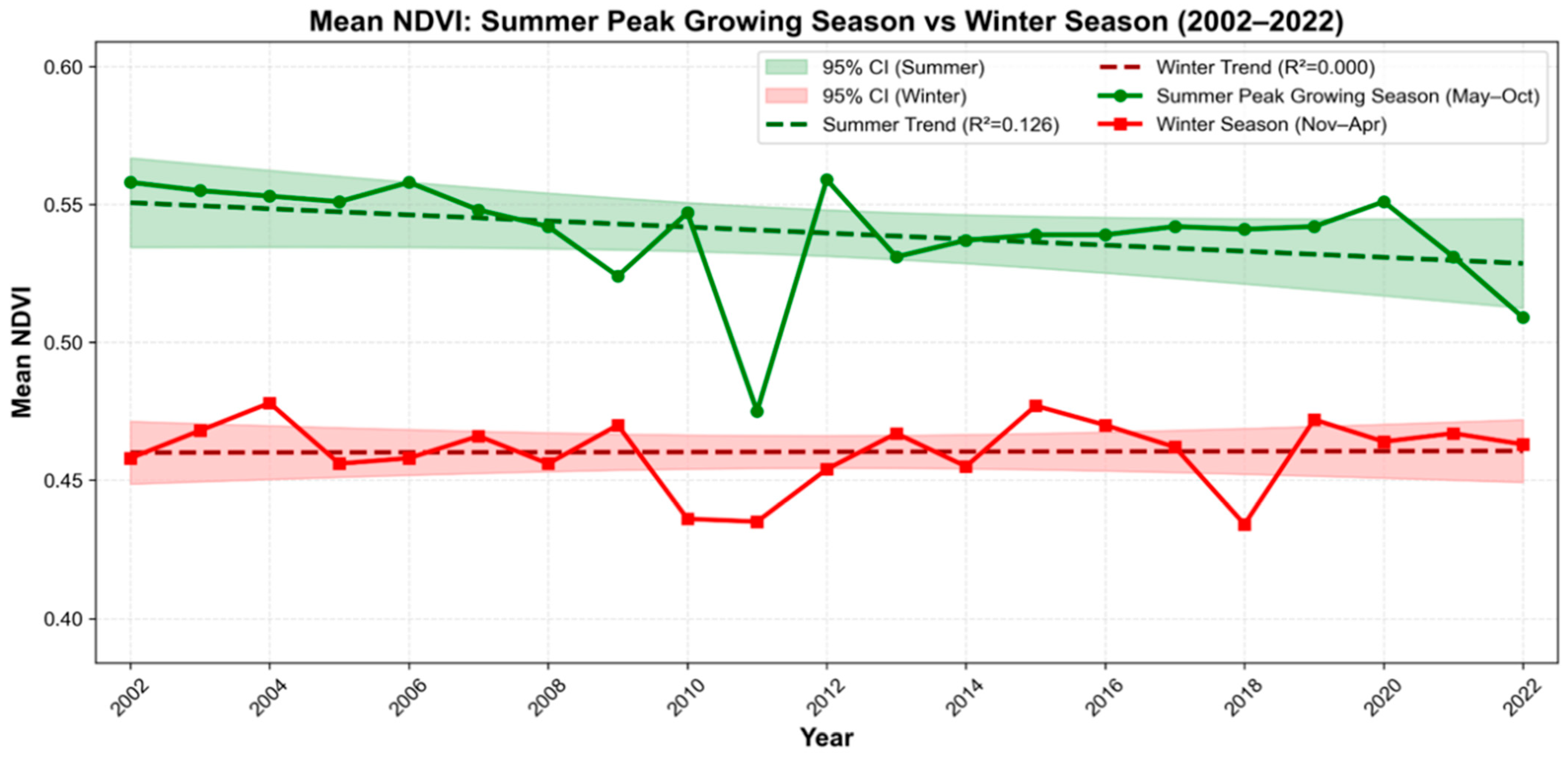
Over the course of the two-decade period, vegetation activity showed distinct seasonal patterns with contrasting trends (Figure 2). The summer peak growing season (May–Oct) exhibited a declining trend of −0.0011 NDVI/year (R2 = 0.126, p = 0.114), equivalent to −0.011 NDVI/decade or approximately 2.0% per decade, with NDVI values decreasing from approximately 0.56 in 2002 to 0.51 in 2022 but this trend is not statistically significant at the 95% confidence level. This decrease is larger than the reduction in vegetated area reported for the Houston area, which was 1% for forest areas and 0.5% for hay/pasture in the years 2001–2019 [25]. In contrast, the winter season (November–April) showed a near-zero trend, maintaining relatively stable NDVI values between 0.43 and 0.48 throughout the study period with no significant long-term change. The summer season exhibited considerably greater interannual variability compared to the winter season, as indicated by the wider 95% confidence intervals (shaded regions in Figure 2). A notable decline occurred in 2011, when summer NDVI dropped to approximately 0.48 due to local drought conditions, followed by a recovery to pre-drought levels by 2013. These results reveal that long-term vegetation decline is driven by changes during the peak growing season, while winter vegetation remains stable in this subtropical region, suggesting that photosynthetic activity and vegetation density are most vulnerable to environmental conditions during the summer months.

4.2. Summer Growing Season Glyoxal Trends (2018–2022)

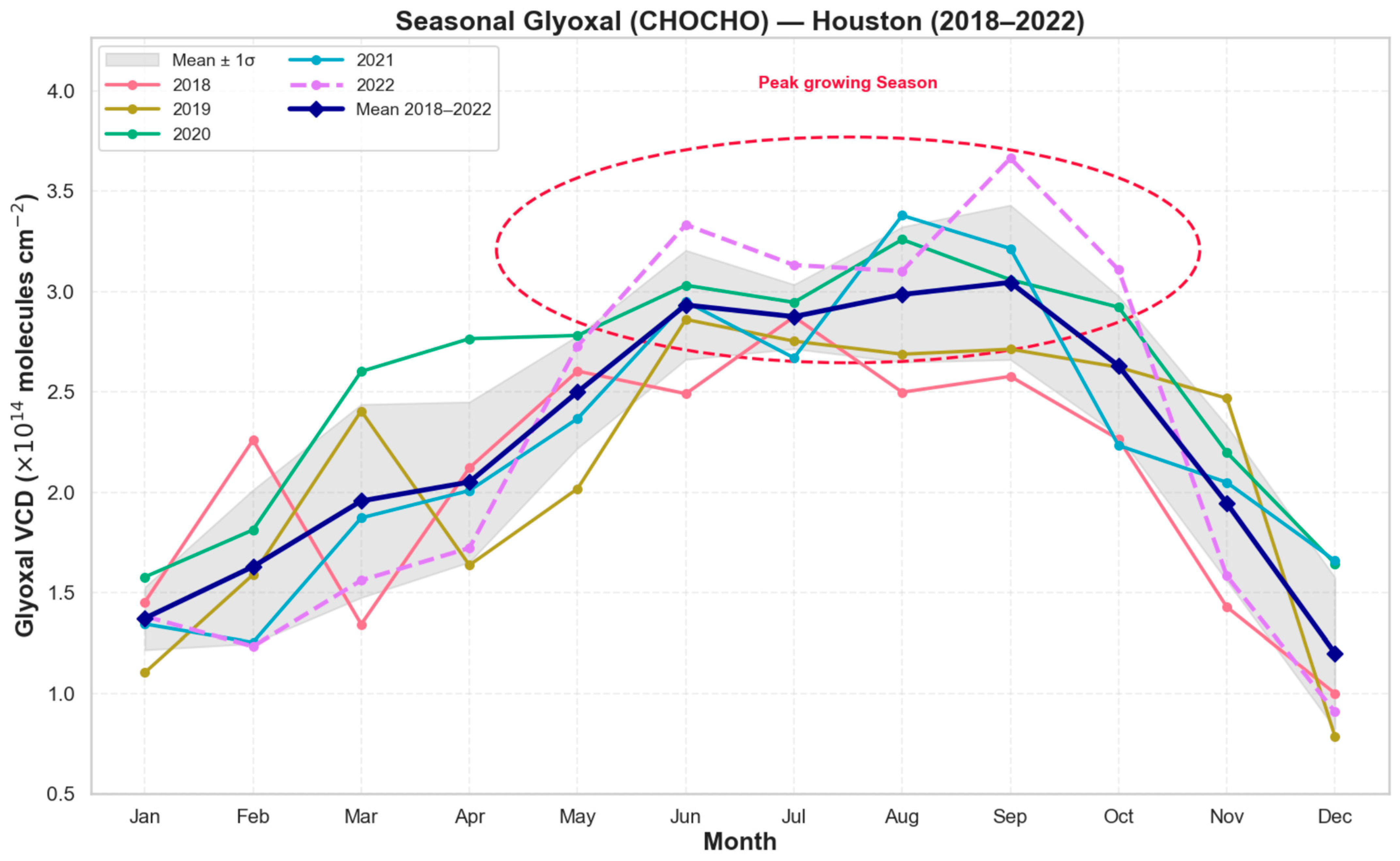
Glyoxal VCD showed clear seasonal periodicity, as seen in Figure 3, with mean winter baseline values (December–February, <1.5 × 10¹⁴ (molecules cm−2) and mean summer peak concentrations (June–September, ~2.5–3.1 × 10¹⁴ (molecules cm−2). Although there is year-to-year variation, the circular area shows the constant summer maximum for all years (2018–2022), with individual years exhibiting peak concentrations during the June–September time frame. The temperature-driven biogenic VOC emissions and increased photochemical oxidation capability typical of Houston’s subtropical summer environment are reflected in this recurrent pattern.
Figure 3 shows the overall glyoxal VCD, produced by both anthropogenic and biogenic VOC precursors. Following the approach for the NDVI analysis shown in Figure 2, the summer growing season is defined as the months May–October. In contrast, the months November–April would be considered the winter baseline. To isolate the fraction of biogenically produced glyoxal ( C H O C H O b i o g ) from the total atmospheric VCD signal, it can be estimated C H O C H O b i o g for each year as follows:
C H O C H O b i o g = C H O C H O G r o w i n g - S e a s o n C H O C H O W i n t e r - B a s e l i n e
where C H O C H O G r o w i n g - S e a s o n is defined by the growing season (May–October) and includes both anthropogenic and biogenic contributions from active vegetation, while C H O C H O W i n t e r - B a s e l i n e represents the winter baseline levels (November–April).
The mean glyoxal VCD for each winter season (November–April) from 2018 to 2022 was calculated, and the annual winter averages were averaged to produce an overall winter baseline of 1.69 ± 0.228 × 10¹⁴ molecules cm−2. This time frame was chosen because glyoxal concentrations are consistently lowest during these months, as shown in Figure 3, mostly due to anthropogenic emissions with little biogenic input from decreased vegetation activity. This represents the upper limit of the anthropogenic contribution to glyoxal. According to [39], global glyoxal production is dominated by biogenic hydrocarbon oxidation (70%), with anthropogenic sources including acetylene (17%) and aromatic compounds (11%) from fossil fuel and industrial emissions. When comparing our winter baseline to the average glyoxal levels during the growing season, the fraction of anthropogenic contribution to the overall glyoxal is about twice (≈58%) the value reported by [39]. However, our study focuses on an urbanized area with high emissions of anthropogenic VOC emissions. During a summertime field campaign, median mixing ratios of isoprene, benzene, and acetylene were about 2.68 ppb, 2.01 ppb, and 1.33 ppb, respectively [17], which would translate into 45% isoprene, 33% benzene, and 22% acetylene contribution to glyoxal production, assuming equal glyoxal formation yields for each VOC.
Strong seasonality is shown in biogenic emissions, which peak in the warm growing months when photosynthetic activity is highest [14]. An analysis of the seasonal variability of VOCs for one site in an industrial area of Houston for the year 2018 showed about eight times higher isoprene mixing ratios in summer vs. wintertime, whereas acetylene levels were about half the values in summer compared to winter [20]. The same study found summertime/wintertime ratios for aromatic compounds ranging from 0.6 to 1.1 among five sites in that area. The two most significant anthropogenic precursors of glyoxal, acetylene and benzene, react with OH slowly, with kOH = 1.22 × 10⁻¹² [cm3 molecule−1 s−1] for benzene [40] and kOH = 7.8 × 10⁻¹³ [cm3 molecule−1 s−1] for acetylene [41].
In contrast to glyoxal produced biogenically, anthropogenic contributions to glyoxal should fluctuate minimally over the year. In the absence of speciated anthropogenic VOC emissions data, the emissions of carbon dioxide (CO2) can be used as a proxy for anthropogenic VOC emissions. A recent study [42] includes daily CO2 emissions data from Houston for the years 2019–2021. Briefly, the lowest CO2 emissions occur in the transition months of April and October (≈150 kt CO2/day), whereas maximum CO2 emissions occur in the months of January and August (≈200 kt CO2/day). For the year 2019, average CO2 emissions were 175 kt CO2/day in the winter months November–April, and 173 kt CO2/day in the growing season months May–October, i.e., a difference of about 1%. Due to COVID regulations in the year 2020, which predominantly impacted ground transportation and aviation, the annual CO2 emissions were about 10% lower; in 2021, they were still 4% lower than in 2019.
A continuous decrease in ambient mixing ratios for both compounds was observed in the time frame 2004–2023 [22], while at the same time the urbanization of the Houston area went on [25].
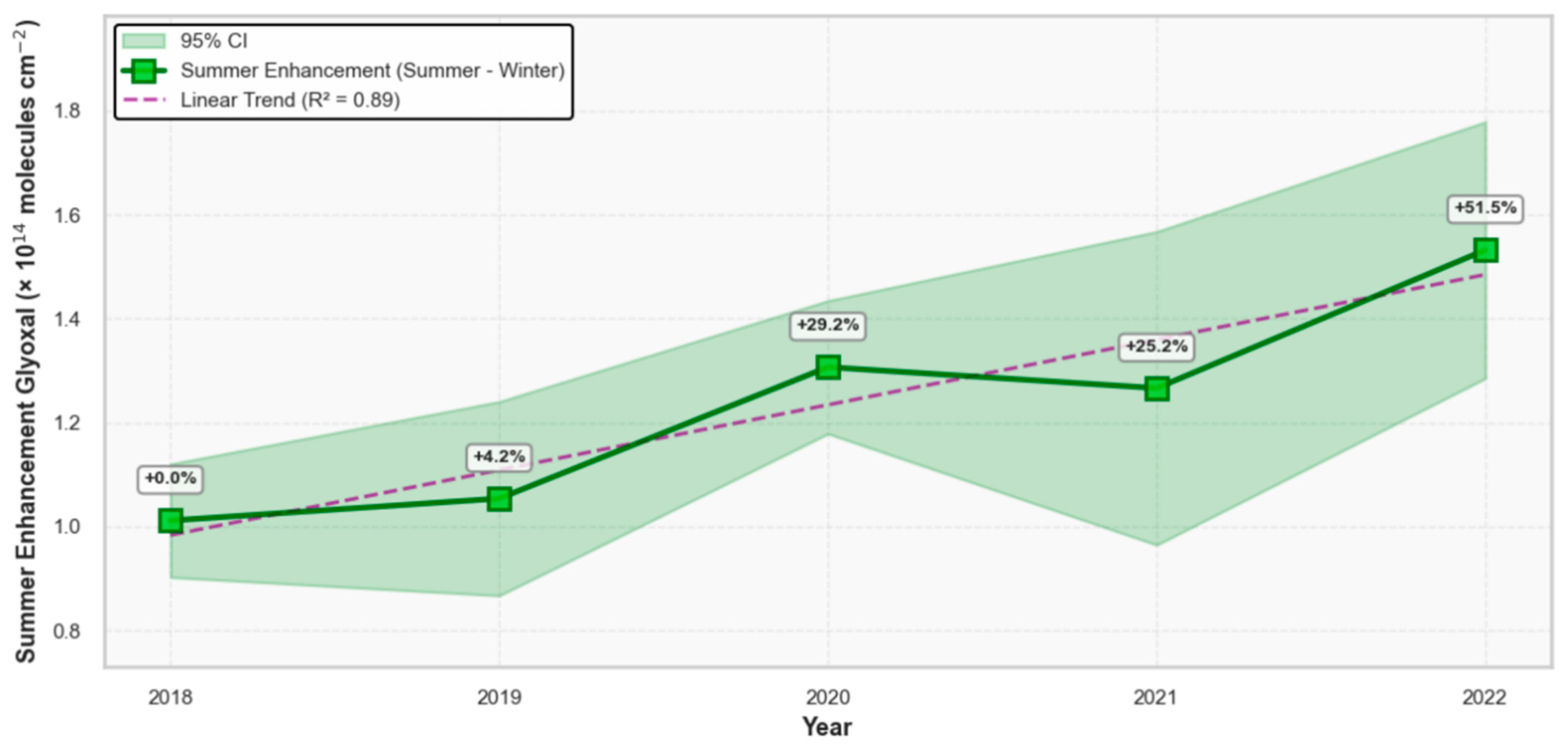
The summer glyoxal enhancement (May–October) in Houston above the winter baseline from 2018 to 2022 is depicted in Figure 4, which demonstrates a strong increasing trend with R2 = 0.89, suggesting good statistical confidence. Summer glyoxal enhancement increased from 1.0 to 1.51 × 10¹⁴ molecules cm−2 throughout this five-year period, a 51% increase above 2018 levels. This significant rise in summer glyoxal enhancement points to higher BVOC emissions during the peak growing season, which is probably caused by more vegetation, warmer temperatures, or more urban greenery in the Houston region. Since glyoxal is a secondary oxidation product of VOCs, rising glyoxal levels may also reflect heightened photochemical activity during summer months.

4.3. Temporal Trends of NDVI and Glyoxal During the Summer Peak Growing Season

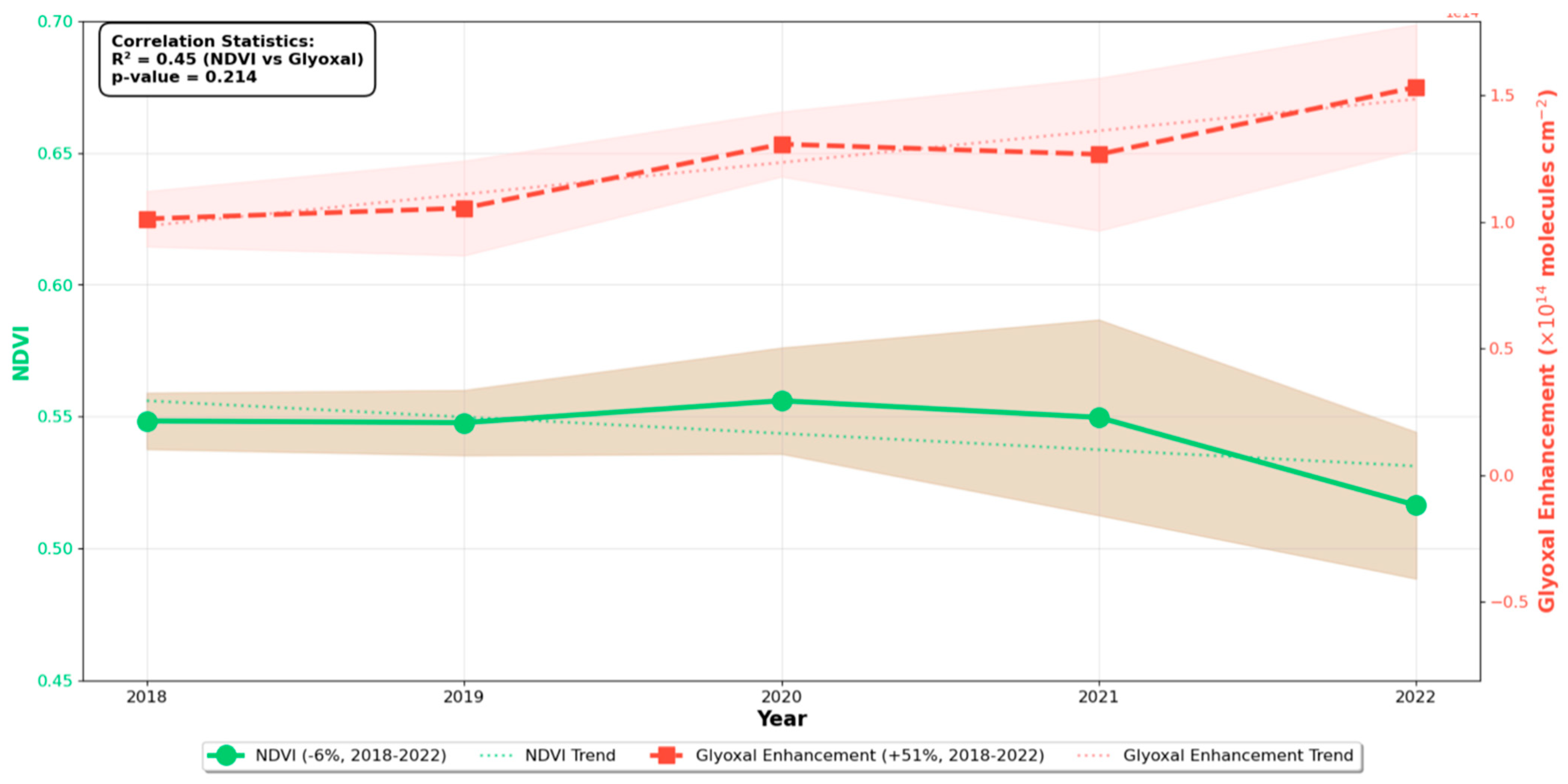
Figure 5 shows the temporal trends of NDVI and glyoxal levels during the summer growing season (May–October) in Houston from 2018 to 2022. From roughly 0.55 in 2018 to 0.52 in 2022, the NDVI dropped by 1.46% year, indicating that vegetation might have become less dense or green over time. The correlation analysis between NDVI and glyoxal summer enhancements yields an R2 value of 0.45, meaning NDVI explains about 45% of the changes in glyoxal, with a p-value of 0.214. This indicates that the statistical strength is insufficient for this association to be deemed significant. Glyoxal levels, on the other hand, rose by almost 13% annually, from roughly 1.0 × 10¹⁴ molecules/cm2 in 2018 to 1.5 × 10¹⁴ molecules/cm2 in 2022. These opposite trends are puzzling because the biogenically produced glyoxal would be expected to increase with more greenery.

4.4. Isoprene and Glyoxal

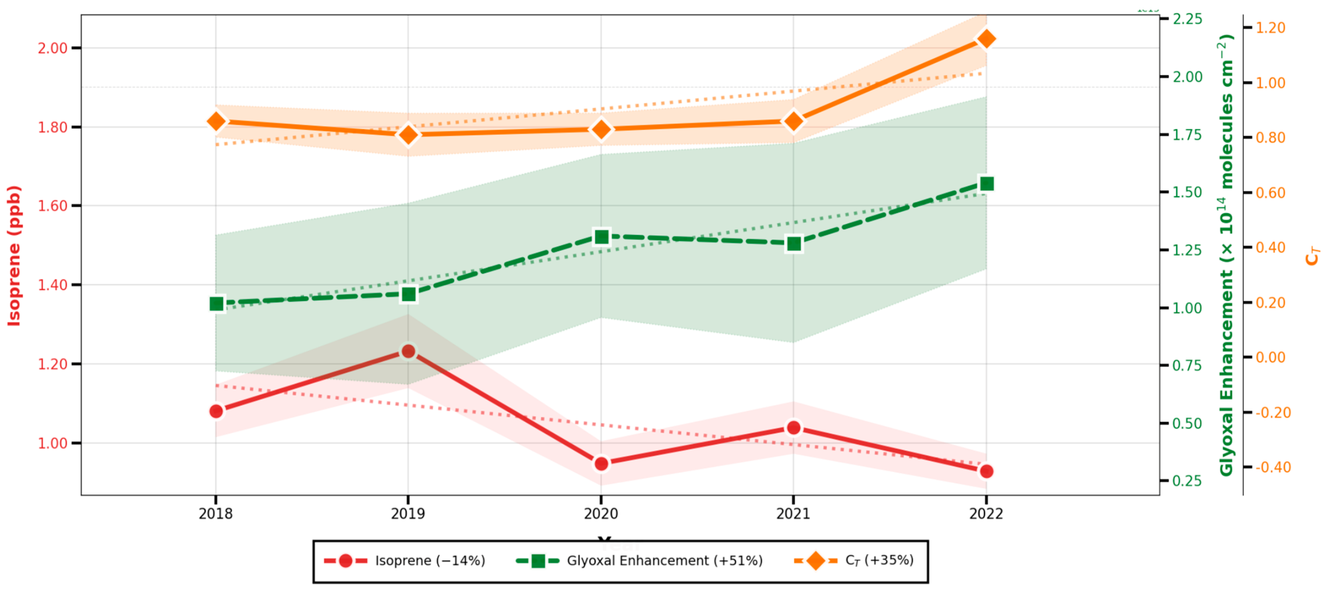
Isoprene is the primary biogenic precursor of glyoxal. The time series of isoprene and glyoxal enhancement in Houston throughout the peak growing season (May–October) between 2018 and 2022 are displayed in Figure 6. There are opposing trends in these two variables.
While isoprene decreased from 1.08 ppb to 0.92 ppb (a 14% decline over 5 years), biogenically produced glyoxal increased by 51% over the same period. The negative correlation between isoprene and glyoxal enhancement (R2 = 0.68, p = 0.088) suggests that other biogenic VOC precursors, enhanced photochemical oxidation, or increased vegetation activity beyond isoprene sources are contributing to the glyoxal increase.
It is known that variations in boundary layer heights (BLHs) impact ambient concentrations of any trace gas in the boundary layer [43], including isoprene, and efforts have been undertaken to account for this [44]. BLHs are determined by surface sensible heat fluxes and/or mechanical shear [45,46]. These processes have been described in multiple analyses, specifically for the area of Houston with its typical coastal Texas prairie land-use/land cover [43,47,48,49,50,51]. Surface heat fluxes in turn are determined by the amount of incoming solar radiation and surface properties (i.e., surface albedo and the soil humidity, which determines the partitioning between latent and sensible heat fluxes). While ambient temperature is also impacted by surface heat fluxes, other processes contribute as well, i.e., advection and radiative properties of the atmosphere through clouds and greenhouse gases. While solar irradiation increased over the longer period 2004–2023, which coincides with decreasing pollution levels in the Houston area, it showed only minor changes during 2018–2022 [52]. In the extreme case of hot and dry conditions, BLHs can reach maximum levels, as surface sensible heat fluxes can largely exceed surface latent heat fluxes and cause enhanced buoyancy, but these conditions can also suppress isoprene emissions due to reduced vegetation activity, as reflected in NDVI. Despite interannual differences in precipitation on the background of long-term increasing precipitation in the Houston area [27], ambient isoprene levels showed a slight decrease during 2018–2022, while temperature increased [22]. Overall, the variability in isoprene is still within the 95% confidence interval and thus not significant for this time period. However, according to [22], this five-year period constitutes one of the highest isoprene levels in the time period 2004–2023. The major finding is the decoupling of increasing glyoxal concentrations from ambient isoprene mixing ratios (Figure 6) and f vegetation greenness, as reflected in the NDVI data (Figure 5).
During the daytime, isoprene reacts with OH and O3. The atmospheric lifetime of isoprene is about 1.4 h, assuming an OH radical concentration of 2.0 × 10⁶ molecules cm−3 as a 12 h daytime average [42,53].
The minimum lifetime of isoprene would occur around noontime due to maximum daytime concentrations of OH in combination with elevated O3. In the study, only the 3 h time period centered around the 13:00 LT satellite overpass during summertime was considered. During this time period, an average OH mixing ratio of 0.5–0.7 pptv, which corresponds to 1.35–1.88 × 10⁷ molecules cm−3, has been observed in Houston in earlier field campaigns [54]. Considering this OH concentration, the noontime isoprene lifetime will only range between 9 and 12 min. At this time of the day, mixing ratios of isoprene represent an equilibrium between emission and removal rates, with transport processes being marginal.
At the same time, isoprene fluxes reach daytime maximum values due to the combination of maximum amount of available photosynthetic active radiation (PAR) and elevated daytime ambient temperatures [55,56,57,58]. It should be noted that emissions of isoprene, not isoprene concentrations, drive glyoxal production. Therefore, our subsequent analysis focuses on the estimate of isoprene emissions rather than on surface isoprene concentrations.
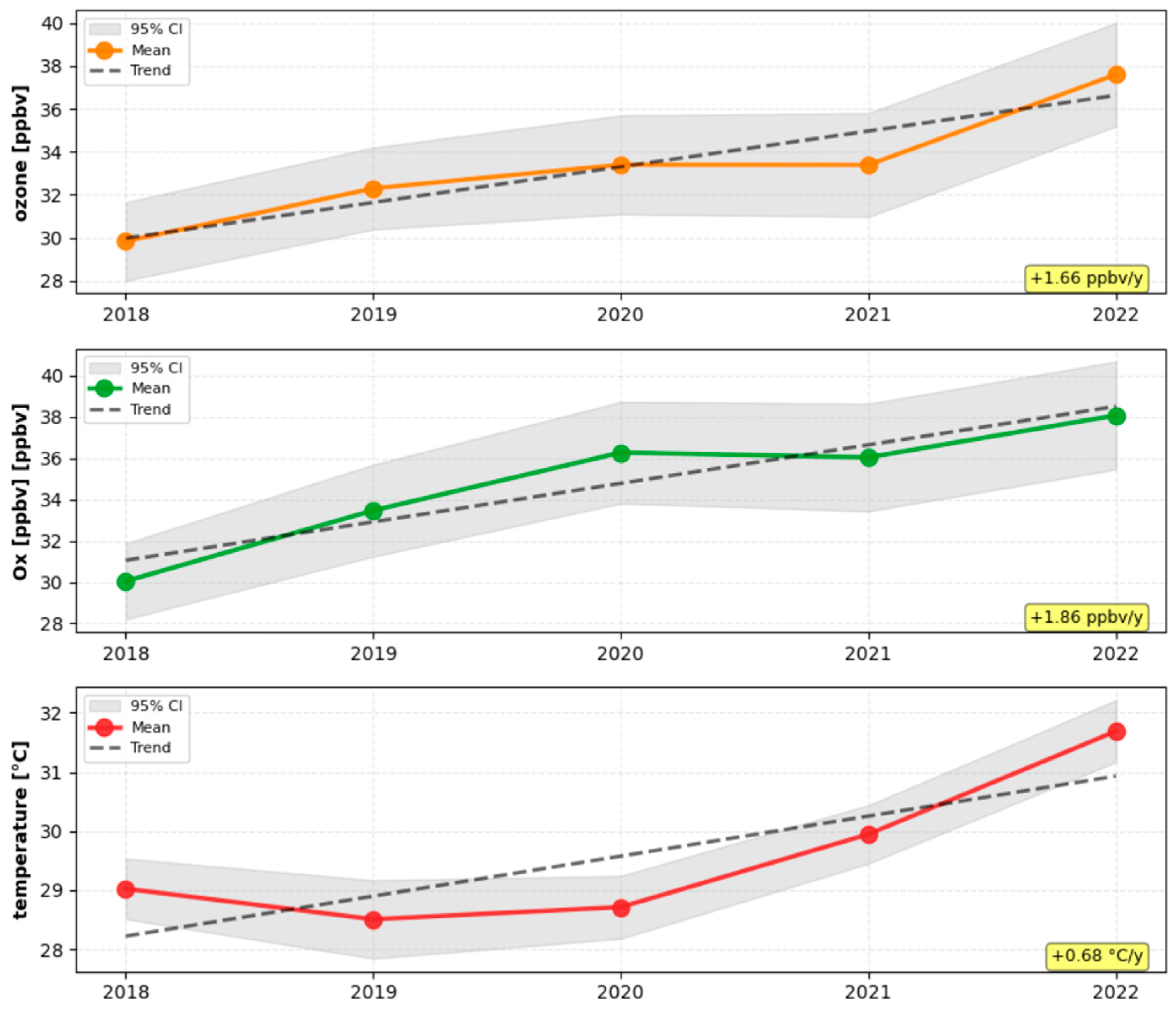
Figure 7 shows annual mean mixing ratios of O3, Ox (Ox: O3 + NO2), and surface temperature with 95% confidence intervals for the growing season noontime period around 13:00 LT. All parameters exhibit significant increasing trends: O3 (+1.66 ppbv/year), Ox (+1.86 ppbv/year), and temperature (+0.68 °C/year). The synchronous increase in O3 and Ox indicates enhanced photochemical oxidant production. The absolute values and the Figure 5 increase in O3 and Ox mixing ratios only differ slightly, making O3 by far the dominant contributor to Ox at this location. Rising temperatures drive increased biogenic emissions, while elevated oxidant levels accelerate isoprene-to-glyoxal conversion, mechanistically linking these trends to the observed increases in glyoxal (Figure 3).
According to [57], isoprene emission I can be estimated as follows:
I = I S × C L × C T
with I S being the isoprene emission at standard conditions, C L describing the light, and C T describing the temperature dependence of isoprene emissions. In this study, only noontime conditions are considered. Thus, only the temperature dependence term C T is taken into account:
C T = exp C T 1 T T S R T S T 1 + exp C T 2 T T M R T S T
with the ideal gas constant R (8.314 J K−1 mol−1), and the standard temperature Ts (303 K). CT1 (95,000 J mol−1), CT2 (230,000 J mol−1), and TM (314 K) are empirically derived values. Based on the temperature time series in Figure 7, there is an increase in isoprene emissions of ≈35 ± 6% in the time period 2018–2022 (Figure 6). The uncertainty of ±6% corresponds to the 95% confidence interval, which is derived by utilizing the recorded temperature values from Figure 7 in the isoprene emission equation.
Figure 6 shows a decrease in ambient isoprene of about 14 ± 10% over the five years 2018–2022. The ±10% uncertainty indicates the 95% confidence interval derived from the trend analysis of ambient isoprene. This decrease suggests removal rates for isoprene, which would compensate for the increased isoprene emissions. According to Figure 7, ozone mixing ratios increased by ≈28 ± 7%, which may cause a corresponding loss of isoprene. The ±7% uncertainty indicates the 95% confidence interval derived from the trend analysis of ozone mixing ratios illustrated in Figure 7. According to a previous study on long-term VOC data, the annual variation in OH might have increased by about 2%/year over the time frame 2004–2023, which also relates to an increase in global radiation of the same magnitude for the daytime periods 11:00–16:00 LT during those years [22]. This would translate into enhanced photochemical processes by ≈10 ± 5% in these five years.
The loss processes for isoprene through OH and O3 altogether increased (≈38%) in the time frame 2018–2022, slightly overcompensating the increased emission of isoprene (≈35%), resulting in an overall decrease in ambient isoprene mixing ratios by ≈−3%. While this value does not match the observed isoprene decrease of −14%, it is within the combined uncertainties. Also, the decrease in isoprene mixing ratios was not found to be statistically significant. On the other hand, the increased isoprene emissions (≈35%) in combination with enhanced photochemically processes induced by a more pronounced annual variation in OH (≈10%) falls short of the observed glyoxal enhancement increase of 51%; it lies again within the combined uncertainties.
Over multiple years, vegetated areas slightly decreased in the Houston area due to ongoing urbanization processes, while in parallel the vegetation greenness as determined by NDVI values also decreased. Nevertheless, based on remote sensing glyoxal data over the Houston area, which have become available for a first set of years, our analysis suggests that the remaining vegetated areas increasingly contributed to the atmospheric glyoxal budget through enhanced isoprene emissions due to changes in ambient temperature and photochemical processes. This supports an analysis of a long-term record of isoprene in the vicinity of the Houston area [22], but expands these results to a larger regional area covered by satellite measurements. While our study is limited to five years, it clearly shows changes in the atmospheric abundance of glyoxal, which should be addressed in more detail once longer datasets become available.
If the vegetation area is shrinking, what is causing the significant rise in atmospheric glyoxal? Two competing hypotheses could explain this pattern: (1) increasing per-plant biogenic emission rates from the remaining vegetation due to elevated temperatures and enhanced metabolic activity, or (2) increased anthropogenic VOC emissions from expanding urban and industrial activities associated with Houston’s rapid growth.

5. Conclusions

An analysis of vegetation greenness based on NDVI data over the Houston, Texas area, over two decades (2002–2022) revealed a slight, albeit steady, decrease of about 2.0% per decade. This happened on the background of continuous urbanization causing fragmentation of vegetated areas of similar magnitude. As vegetation is a dominant source for atmospheric glyoxal through the emission of isoprene, the first available tropospheric column data for glyoxal from TROPOMI were analyzed for the time period 2018–2022 over Houston. The research findings show an unusual pattern in Houston: while vegetation greenness stayed relatively stable or decreased slightly, glyoxal emissions increased significantly by ≈51 ± 20% over the five-year period. This contradicts what is normally expected, where more vegetation should produce more glyoxal. Instead, less active vegetation would be causing more glyoxal. Even more surprising, observation of isoprene mixing ratios during the satellite overpasses decreased by 14 ± 10% over these five years, when normally isoprene converts to glyoxal initiated by reactions with the hydroxyl radical (OH) and the two, isoprene and glyoxal, would be expected to show similar trends.
Additional data including ozone and ambient temperature reveal important environmental changes: temperature increased by 0.68 °C per year, while ozone mixing ratios increased by ≈28. Increased ambient noontime temperatures were found to enhance the temperature-dependent isoprene emission term CT by about ≈35, while higher levels of ozone may have reduced ambient isoprene mixing ratios through reactions of ozone with isoprene. Earlier studies indicated a 2.1%/year increase in the annual variation in OH based on 20 years of observations of volatile organic compounds in the vicinity of Houston. It is concluded that Houston’s slightly declining vegetation has been emitting more isoprene due to increasing temperature and, in combination with higher oxidant levels, has been causing more glyoxal per unit area. Plants can emit elevated levels of volatile organic compounds even when they are less green and healthy. Furthermore, the rising temperatures and oxidant concentrations create favorable atmospheric conditions that enhance glyoxal formation through chemical reactions. The combination of changes in vegetation emission behavior, rising temperatures, and increased oxidative conditions is driving the substantial increase in atmospheric glyoxal abundance observed over Houston.
This study is based on a first and limited glyoxal dataset of five years. Nevertheless, this dataset reveals a significant increase in biogenically driven glyoxal over the Houston area. Future studies with longer glyoxal records should gain more insights into the intrinsic isoprene–glyoxal relations in a changing environment.

Author Contributions

Conceptualization, B.R.; Methodology, B.R.; Software, S.B.; Validation, B.R.; Formal analysis, S.B.; Investigation, S.B. and B.R.; Resources, B.R.; Data curation, B.R.; Writing—original draft, S.B.; Writing—review & editing, B.R.; Visualization, S.B.; Supervision, B.R. All authors have read and agreed to the published version of the manuscript.

Funding

This research received no external funding.

Institutional Review Board Statement

Not applicable.

Informed Consent Statement

Not applicable.

Data Availability Statement

The glyoxal data supporting the findings of the study are publicly available at https://glyretro.aeronomie.be/index.php/component/users/?view=login&Itemid=101 (accessed on 1 September 2025).

Acknowledgments

The author gratefully acknowledges the guidance and support of the research supervisor throughout this study. Support from the University of Houston is also sincerely appreciated for providing the academic environment and resources that enabled this research.

Conflicts of Interest

The authors declare no conflict of interest.

References

  1. Chen, Y.; Su, W.; Wang, Z.; Huo, Y.; Xun, S.; Chen, X.; He, B.; Liu, C. Application of Space-Based Glyoxal Observation for Estimating Global Nonmethane Volatile Organic Compounds Emissions from Urban Sources and Biomass Burning. Environ. Sci. Technol. Lett. 2025, 12, 209–215. [Google Scholar] [CrossRef] [Scilit]
  2. Lun, X.; Lin, Y.; Chai, F.; Fan, C.; Li, H.; Liu, J. Reviews of Emission of Biogenic Volatile Organic Compounds (BVOCs) in Asia. J. Environ. Sci. 2020, 95, 266–277. [Google Scholar] [CrossRef] [Scilit]
  3. Fu, T.-M.; Jacob, D.J.; Wittrock, F.; Burrows, J.P.; Vrekoussis, M.; Henze, D.K.; Fu, C.; Jacob, D.J.; Wittrock, F.; Burrows, J.P.; et al. Global Budgets of Atmospheric Glyoxal and Methylglyoxal, and Implications for Formation of Secondary Organic Aerosols. J. Geophys. Res. Atmos. 2008, 113, 15303. [Google Scholar] [CrossRef] [Scilit]
  4. Volkamer, R.; Platt, U.; Wirtz, K. Primary and Secondary Glyoxal Formation from Aromatics: Experimental Evidence for the Bicycloalkyl−Radical Pathway from Benzene, Toluene, and p-Xylene. J. Phys. Chem. A 2001, 105, 7865–7874. [Google Scholar] [CrossRef] [Scilit]
  5. Nishino, N.; Arey, J.; Atkinson, R. Formation Yields of Glyoxal and Methylglyoxal from the Gas-Phase OH Radical-Initiated Reactions of Toluene, Xylenes, and Trimethylbenzenes as a Function of NO2 Concentration. J. Phys. Chem. A 2010, 114, 10140–10147. [Google Scholar] [CrossRef] [Scilit]
  6. Chan Miller, C.; Jacob, D.J.; Marais, E.A.; Yu, K.; Travis, K.R.; Kim, P.S.; Fisher, J.A.; Zhu, L.; Wolfe, G.M.; Hanisco, T.F.; et al. Glyoxal Yield from Isoprene Oxidation and Relation to Formaldehyde: Chemical Mechanism, Constraints from SENEX Aircraft Observations, and Interpretation of OMI Satellite Data. Atmos. Chem. Phys. 2017, 17, 8725–8738. [Google Scholar] [CrossRef] [Scilit]
  7. Kesselmeier, J.; Staudt, M. Biogenic Volatile Organic Compounds (VOC): An Overview on Emission, Physiology and Ecology. J. Atmos. Chem. 1999, 33, 23–88. [Google Scholar] [CrossRef] [Scilit]
  8. Sharkey, T.D.; Wiberley, A.E.; Donohue, A.R. Isoprene Emission from Plants: Why and How. Ann. Bot. 2008, 101, 5–18. [Google Scholar] [CrossRef] [Scilit]
  9. Fitzky, A.C.; Sandén, H.; Karl, T.; Fares, S.; Calfapietra, C.; Grote, R.; Saunier, A.; Rewald, B. The Interplay Between Ozone and Urban Vegetation—BVOC Emissions, Ozone Deposition, and Tree Ecophysiology. Front. For. Glob. Change 2019, 2, 50. [Google Scholar] [CrossRef] [Scilit]
  10. Gu, S.; Guenther, A.; Faiola, C. Effects of Anthropogenic and Biogenic Volatile Organic Compounds on Los Angeles Air Quality. Environ. Sci. Technol. 2021, 55, 12191–12201. [Google Scholar] [CrossRef] [Scilit] [PubMed]
  11. Ren, Y.; Qu, Z.; Du, Y.; Xu, R.; Ma, D.; Yang, G.; Shi, Y.; Fan, X.; Tani, A.; Guo, P.; et al. Air Quality and Health Effects of Biogenic Volatile Organic Compounds Emissions from Urban Green Spaces and the Mitigation Strategies. Environ. Pollut. 2017, 230, 849–861. [Google Scholar] [CrossRef] [Scilit]
  12. Ma, M.; Gao, Y.; Wang, Y.; Zhang, S.; Ruby Leung, L.; Liu, C.; Wang, S.; Zhao, B.; Chang, X.; Su, H.; et al. Substantial Ozone Enhancement over the North China Plain from Increased Biogenic Emissions Due to Heat Waves and Land Cover in Summer 2017. Atmos. Chem. Phys. 2019, 19, 12195–12207. [Google Scholar] [CrossRef] [Scilit]
  13. Chan Miller, C.; Jacob, D.J.; González Abad, G.; Chance, K. Hotspot of Glyoxal over the Pearl River Delta Seen from the OMI Satellite Instrument: Implications for Emissions of Aromatic Hydrocarbons. Atmos. Chem. Phys. 2016, 16, 4631–4639. [Google Scholar] [CrossRef] [Scilit]
  14. Guenther, A. Seasonal and Spatial Variations in Natural Volatile Organic Compound Emissions-Guenther-1997-Ecological Applications-Wiley Online Library. Ecol. Appl. 1997, 7, 34–45. [Google Scholar] [CrossRef]
  15. Yang, Y.; Sun, F.; Chen, Y.; Yang, S.; Dai, Y.; Qin, Y.; Zhang, N.; Shu, Z.; Yan, H.; Ge, X.; et al. Impact of Temperature on the Biogenic Volatile Organic Compound (BVOC) Emissions in China: A Review. J. Environ. Sci. 2026, 159, 649–660. [Google Scholar] [CrossRef] [Scilit] [PubMed]
  16. Zuazo, I.; Torre-Pascual, E.; García, J.A. Evaluation of Satellite Vegetation Indices for BVOCs Emission Modelling. Case Study: Basque Country. In Springer Proceedings in Complexity; Springer: Cham, Switzerland, 2022; pp. 303–308. [Google Scholar]
  17. Leuchner, M.; Rappenglück, B. VOC Source–Receptor Relationships in Houston During TexAQS-II. Atmos. Environ. 2010, 44, 4056–4067. [Google Scholar] [CrossRef] [Scilit]
  18. Rappenglück, B.; Lubertino, G.; Alvarez, S.; Golovko, J.; Czader, B.; Ackermann, L. Radical Precursors and Related Species from Traffic as Observed and Modeled at an Urban Highway Junction. J. Air Waste Manag. Assoc. 2013, 63, 1270–1286. [Google Scholar] [CrossRef] [Scilit]
  19. Ahmed, M.; Rappenglück, B.; Das, S.; Chellam, S. Source Apportionment of Volatile Organic Compounds, CO, SO2 and Trace Metals in a Complex Urban Atmosphere. Environ. Adv. 2021, 6, 100127. [Google Scholar] [CrossRef] [Scilit]
  20. Sadeghi, B.; Pouyaei, A.; Choi, Y.; Rappenglueck, B. Influence of Seasonal Variability on Source Characteristics of VOCs at Houston Industrial Area. Atmos. Environ. 2022, 277, 119077. [Google Scholar] [CrossRef] [Scilit]
  21. Li, G.; Zhang, R.; Fan, J.; Tie, X. Impacts of Biogenic Emissions on Photochemical Ozone Production in Houston, Texas. J. Geophys. Res. Atmos. 2007, 112, 10309. [Google Scholar] [CrossRef] [Scilit]
  22. Ahmed, M.; Ahmad, M.; Rappenglueck, B. Twenty Years (2004–2023) Observation of Non-Methane Hydrocarbons in a Subtropical Coastal Environment—Indications of Increased Isoprene Emissions. Atmos. Environ. 2025, 343, 120993. [Google Scholar] [CrossRef] [Scilit]
  23. Census Bureau United States Census. Available online: https://www.census.gov/popclock/ (accessed on 14 November 2025).
  24. Texas Urban Planning Agency Growth Challenges and Opportunities in the Texas Triangle. Available online: https://texasup.org/uncategorized/growth-challenges-and-opportunities-in-the-texas-triangle/?utm_source=chatgpt.com (accessed on 14 November 2025).
  25. Madeline, S. The Impact of a Rapidly Growing Urban Area on Changing Precipitation Patterns; University of Houston: Houston, TX, USA, 2023. [Google Scholar]
  26. Li, Z.; Li, X.; Wang, Y.; Quiring, S.M. Impact of Climate Change on Precipitation Patterns in Houston, Texas, USA. Anthropocene 2019, 25, 100193. [Google Scholar] [CrossRef] [Scilit]
  27. Statkewicz, M.D.; Talbot, R.; Rappenglueck, B. Changes in Precipitation Patterns in Houston, Texas. Environ. Adv. 2021, 5, 100073. [Google Scholar] [CrossRef] [Scilit]
  28. Statkewicz, M.D.; Rappenglueck, B. A Comparative Analysis of the Sea Breeze on the Texas Gulf Coast and Its Impact on Precipitation. Urban Clim. 2023, 49, 101568. [Google Scholar] [CrossRef] [Scilit]
  29. Gu, J.; Li, X.; Huang, C.; Okin, G.S. A Simplified Data Assimilation Method for Reconstructing Time-Series MODIS NDVI Data. Adv. Space Res. 2009, 44, 501–509. [Google Scholar] [CrossRef] [Scilit]
  30. Yengoh, G.T.; Dent, D.; Olsson, L.; Tengberg, A.E.; Tucker, C.J., III. Use of the Normalized Difference Vegetation Index (NDVI) to Assess Land Degradation at Multiple Scales: Current Status, Future Trends, and Practical Considerations; Springer: Berlin/Heidelberg, Germany, 2015. [Google Scholar]
  31. Mokarram, M.; Soleimanpour, L.; Hojati, M.; Mokarram, M. Applied Remote Sensing for Determination of Vegetation Index. J. Environ. 2016, 5, 19–23. [Google Scholar]
  32. Zhai, Y.; Roy, D.P.; Martins, V.S.; Zhang, H.K.; Yan, L.; Li, Z. Conterminous United States Landsat-8 Top of Atmosphere and Surface Reflectance Tasseled Cap Transformation Coefficients. Remote Sens. Environ. 2022, 274, 112992. [Google Scholar] [CrossRef] [Scilit]
  33. Worku, M.A.; Feyisa, G.L.; Beketie, K.T.; Garbolino, E. Spatiotemporal Dynamics of Vegetation in Response to Climate Variability in the Borana Rangelands of Southern Ethiopia. Front. Earth Sci. 2023, 11, 991176. [Google Scholar] [CrossRef] [Scilit]
  34. Kleipool, Q.; Ludewig, A.; Babic, L.; Bartstra, R.; Braak, R.; Dierssen, W.; Dewitte, P.J.; Kenter, P.; Landzaat, R.; Leloux, J.; et al. Pre-Launch Calibration Results of the TROPOMI Payload on-Board the Sentinel-5 Precursor Satellite. Atmos. Meas. Tech. 2018, 11, 6439–6479. [Google Scholar] [CrossRef] [Scilit]
  35. Woiwode, W.; Oelhaf, H.; Gulde, T.; Piesch, C.; Maucher, G.; Ebersoldt, A.; Keim, C.; Höpfner, M.; Khaykin, S.; Ravegnani, F.; et al. MIPAS-STR measurements in the Arctic UTLS in winter/spring 2010: Instrument characterization, retrieval and validation. Atmos. Meas. Tech. 2012, 5, 1205–1228. [Google Scholar] [CrossRef] [Scilit]
  36. Lerot, C.; Hendrick, F.; Van Roozendael, M.; Alvarado, L.M.A.; Richter, A.; De Smedt, I.; Theys, N.; Vlietinck, J.; Yu, H.; Van Gent, J.; et al. Glyoxal Tropospheric Column Retrievals from TROPOMI-Multi-Satellite Intercomparison and Ground-Based Validation. Atmos. Meas. Tech. 2021, 14, 7775–7807. [Google Scholar] [CrossRef] [Scilit]
  37. Chen, Y.; Su, W.; Xing, C.; Yin, H.; Lin, H.; Zhang, C.; Liu, H.; Hu, Q.; Liu, C. Kilometer-Level Glyoxal Retrieval via Satellite for Anthropogenic Volatile Organic Compound Emission Source and Secondary Organic Aerosol Formation Identification. Remote Sens. Environ. 2022, 270, 112852. [Google Scholar] [CrossRef] [Scilit]
  38. Stutz, J.; Wong, K.W.; Lawrence, L.; Ziemba, L.; Flynn, J.H.; Rappenglück, B.; Lefer, B. Nocturnal NO3 Radical Chemistry in Houston, TX. Atmos. Environ. 2010, 44, 4099–4106. [Google Scholar] [CrossRef] [Scilit]
  39. Myriokefalitakis, S.; Vrekoussis, M.; Tsigaridis, K.; Wittrock, F.; Richter, A.; Brühl, C.; Volkamer, R.; Burrows, J.P.; Kanakidou, M. The Influence of Natural and Anthropogenic Secondary Sources on the Glyoxal Global Distribution. Atmos. Chem. Phys. 2008, 8, 4965–4981. [Google Scholar] [CrossRef] [Scilit]
  40. Atkinson, R.; Arey, J. Atmospheric Degradation of Volatile Organic Compounds. Chem. Rev. 2003, 103, 4605–4638. [Google Scholar] [CrossRef] [Scilit] [PubMed]
  41. Atkinson, R.; Baulch, D.L.; Cox, R.A.; Crowley, J.N.; Hampson, R.F.; Hynes, R.G.; Jenkin, M.E.; Rossi, M.J.; Troe, J. Evaluated Kinetic and Photochemical Data for Atmospheric Chemistry: Volume II—Gas Phase Reactions of Organic Species. Atmos. Chem. Phys. 2006, 6, 3625–4055. [Google Scholar] [CrossRef] [Scilit]
  42. Huo, D.; Huang, X.; Dou, X.; Ciais, P.; Li, Y.; Deng, Z.; Wang, Y.; Cui, D.; Benkhelifa, F.; Sun, T.; et al. Carbon Monitor Cities: Near-real-time daily estimates of CO2 emissions from 1500 cities worldwide. Sci. Data 2022, 9, 533. [Google Scholar] [CrossRef] [Scilit] [PubMed]
  43. Cuchiara, G.C.; Li, X.; Carvalho, J.; Rappenglück, B. Intercomparison of Planetary Boundary Layer Parameterization and Its Impacts on Surface Ozone Concentration in the WRF/Chem Model for a Case Study in Houston/Texas. Atmos. Environ. 2014, 96, 175–185. [Google Scholar] [CrossRef] [Scilit]
  44. Akther, T.; Rappenglueck, B.; Osibanjo, O.; Retama, A.; Rivera-Hernández, O. Ozone Precursors and Boundary Layer Meteorology Before and During a Severe Ozone Episode in Mexico City. Chemosphere 2023, 318, 137978. [Google Scholar] [CrossRef] [Scilit]
  45. Arya, S.P. Air Pollution Meteorology and Dispersion; Oxford University Press: Oxford, UK, 1999. [Google Scholar]
  46. Stull, R.B. An Introduction to Boundary Layer Meteorology; Springer Science+Business Media: Dordrecht, The Netherlands, 2012; Volume 13. [Google Scholar] [CrossRef] [Scilit]
  47. Cuchiara, G.C.; Rappenglück, B. Simulating the Influence of Convective Decay Parameterization for a Case Study in Houston, TX. Atmos. Environ. 2019, 204, 68–77. [Google Scholar] [CrossRef] [Scilit]
  48. Li, X.; Rappenglueck, B. A Study of Model Nighttime Ozone Bias in Air Quality Modeling. Atmos. Environ. 2018, 195, 210–228. [Google Scholar] [CrossRef] [Scilit]
  49. Cuchiara, G.C.; Rappenglück, B. Performance Analysis of WRF and LES in Describing the Evolution and Structure of the Planetary Boundary Layer. Environ. Fluid Mech. 2018, 18, 1257–1273. [Google Scholar] [CrossRef] [Scilit]
  50. Cuchiara, G.C.; Rappenglück, B. Single-Column Model and Large Eddy Simulation of the Evening Transition in the Planetary Boundary Layer. Environ. Fluid Mech. 2017, 17, 777–798. [Google Scholar] [CrossRef] [Scilit]
  51. Wilmot, C.S.M.; Rappenglück, B.; Li, X.; Cuchiara, G. MM5 v3.6.1 and WRF v3.5.1 Model Comparison of Standard and Surface Energy Variables in the Development of the Planetary Boundary Layer. Geosci. Model Dev. 2014, 7, 2693–2707. [Google Scholar] [CrossRef] [Scilit]
  52. Anshika; Soneye-Arogundade, O.O.; Rappenglück, B. Evaluating Diffuse Radiation Models: A 20-Year Case Study in Houston and Implications for Solar Panel Tilt Optimization. Theor. Appl. Clim. 2026. revised. [Google Scholar]
  53. Atkinson, R.; Arey, J. Gas-Phase Tropospheric Chemistry of Biogenic Volatile Organic Compounds: A Review. Atmos. Environ. 2003, 37, 197–219. [Google Scholar] [CrossRef] [Scilit]
  54. Mao, J.; Ren, X.; Chen, S.; Brune, W.H.; Chen, Z.; Martinez, M.; Harder, H.; Lefer, B.; Rappenglück, B.; Flynn, J.; et al. Atmospheric oxidation capacity in the summer of Houston 2006: Comparison with summer measurements in other metropolitan studies. Atmos. Environ. 2010, 44, 4107–4115. [Google Scholar] [CrossRef] [Scilit]
  55. Forkel, R.; Klemm, O.; Graus, M.; Rappenglück, B.; Stockwell, W.R.; Grabmer, W.; Held, A.; Hansel, A.; Steinbrecher, R. Trace Gas Exchange and Gas Phase Chemistry in a Norway Spruce Forest: A Study with a Coupled 1-Dimensional Canopy Atmospheric Chemistry Emission Model. Atmos. Environ. 2006, 40, 28–42. [Google Scholar] [CrossRef] [Scilit]
  56. Guenther, A.B.; Jiang, X.; Heald, C.L.; Sakulyanontvittaya, T.; Duhl, T.; Emmons, L.K.; Wang, X. The Model of Emissions of Gases and Aerosols from Nature Version 2.1 (MEGAN2.1): An extended and updated framework for modeling biogenic emissions. Geosci. Model Dev. 2012, 5, 1471–1492. [Google Scholar] [CrossRef] [Scilit]
  57. Guenther, A.B.; Zimmerman, P.R.; Harley, P.C.; Monson, R.K.; Fall, R. Isoprene and Monoterpene Emission Rate Variability: Model Evaluations and Sensitivity Analyses. J. Geophys. Res. Atmos. 1993, 98, 12609–12617. [Google Scholar] [CrossRef] [Scilit]
  58. Guenther, A.; Hewitt, C.N.; Erickson, D.; Fall, R.; Geron, C.; Graedel, T.; Harley, P.; Klinger, L.; Lerdau, M.; McKay, W.A.; et al. A global model of natural volatile organic compound emissions. J. Geophys. Res. Atmos. 1995, 100, 8873–8892. [Google Scholar] [CrossRef] [Scilit]
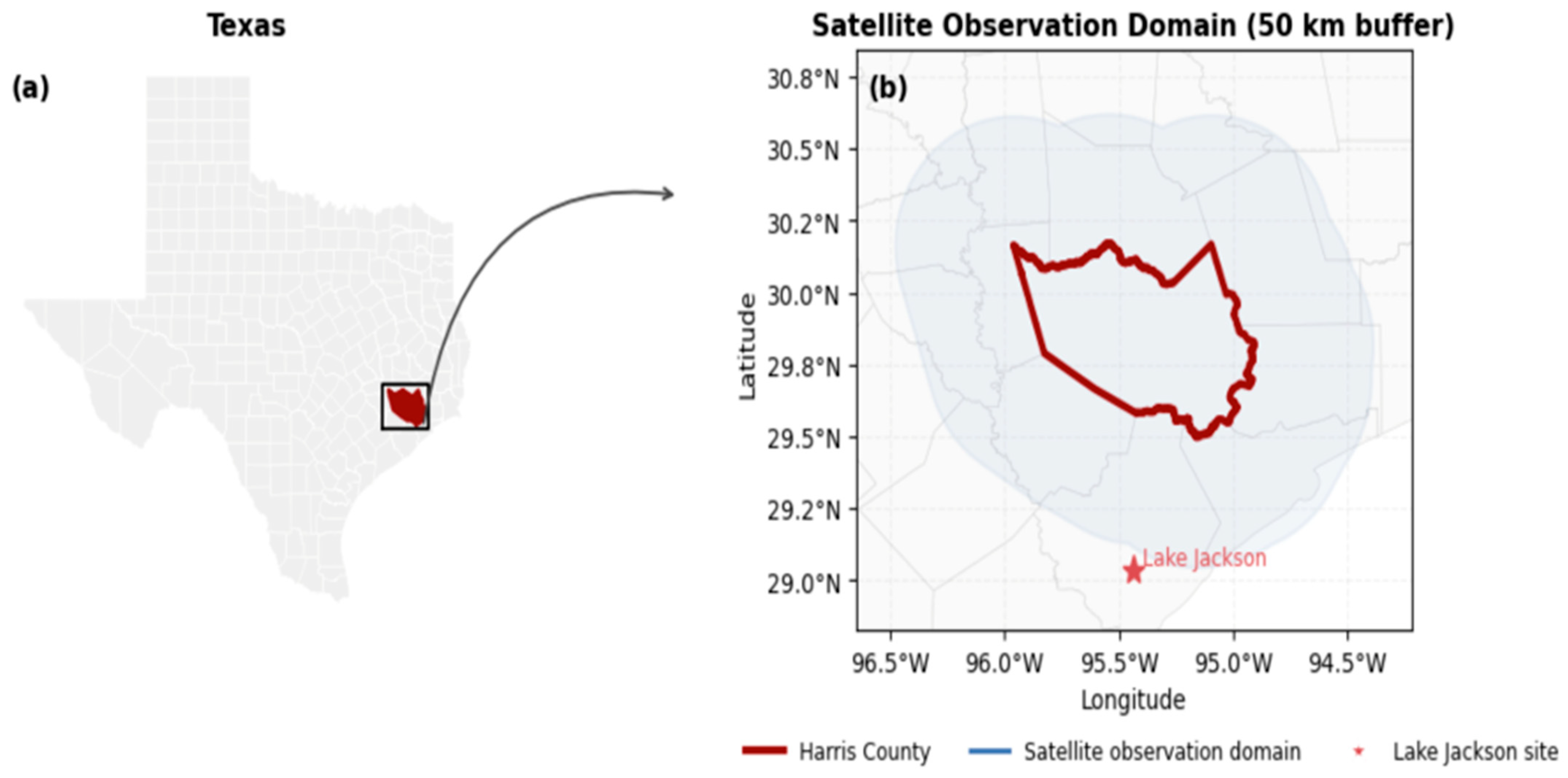
Figure 1. Study area and satellite observation domain. (a) Harris County location in Texas; (b) County boundary, 50 km observation domain, and Lake Jackson site.
Atmosphere 17 00100 g001
Figure 2. Yearly average NDVI comparison between the peak summer (May–October) and winter (November–April) seasons from 2002 to 2022.
Atmosphere 17 00100 g002
Figure 3. Annual variation in glyoxal VCD over Houston (2018–2022). Encircled is the summertime enhancement of glyoxal.
Atmosphere 17 00100 g003
Figure 4. Annual mean VCD glyoxal over Houston during the summer growing season (May–October) from 2018 to 2022. The percentages indicate the increase in glyoxal with regard to the preceding year. The green-shaded area represents the 95% confidence interval around the linear trend line.
Atmosphere 17 00100 g004
Figure 5. Temporal trends of NDVI and glyoxal enhancement during the summer peak growing season (May–October) over Houston in the time frame 2018–2022. The shaded areas represent 95% confidence intervals for NDVI (green/tan) and glyoxal enhancement (red/pink) trend lines.
Atmosphere 17 00100 g005
Figure 6. Temporal trends of isoprene, glyoxal enhancement, and CT during the peak growing season (May–October) in the time frame 2018–2022.
Atmosphere 17 00100 g006
Figure 7. Temporal trends in ozone, Ox, and temperature in the time frame 2018–2020.
Atmosphere 17 00100 g007
Table 1. MODIS NDVI product.
ItemMODIS NDVI Product
File nameVegetation Indices 16-Day L3 Global 250 m Version 6
Spatial resolution250 m
Input imageMODIS/TERRA MOD09Q1
Composition16-day
Data (years)2002–2022
Seasonal averages were divided into two periods: the summer peak growing season (May–October), representing peak vegetation activity, and the dormant season ‘winter growing season’ (November–April), when vegetation growth is minimal.
Table 2. TROPOMI Glyoxal Data.
Parameter Description
Satellite NameTROPOMI (Tropospheric Monitoring Instrument) onboard the Sentinel-5 Precursor satellite
Data Period UsedJanuary 2018–December 2022
Target VariableTropospheric Glyoxal (C2H2O2),
Vertical Column Density—VCD (molecules/cm2)
Spatial Resolution7 × 3.5 km2 (improved to 5 × 3.5 km2 since August 2019)
Disclaimer/Publisher’s Note: The statements, opinions and data contained in all publications are solely those of the individual author(s) and contributor(s) and not of MDPI and/or the editor(s). MDPI and/or the editor(s) disclaim responsibility for any injury to people or property resulting from any ideas, methods, instructions or products referred to in the content.