Abstract
Knowledge of ionospheric plasma altitudinal distribution is crucial for the effective operation of radio wave propagation, communication, and navigation systems. High-frequency sounding radars—ionosondes—provide unbiased benchmark measurements of ionospheric plasma density due to a direct relationship between the frequency of sound waves and ionospheric electron density. But ground-based ionosonde observations are limited by the F2 layer peak height and cannot probe the topside ionosphere. GNSS Radio Occultation (RO) onboard Low-Earth-Orbiting satellites can provide measurements of plasma distribution from the lower ionosphere up to satellite orbit altitudes (~500–600 km). The main goal of this study is to investigate opportunities to obtain full observation-based ionospheric electron density profiles (EDPs) by combining advantages of ground-based ionosondes and GNSS RO. We utilized the high-rate Ebre and El Arenosillo ionosonde observations and COSMIC-2 RO EDPs colocated over the ionosonde’s area of operation. Using two types of ionospheric remote sensing techniques, we demonstrated how to create the combined ionospheric EDPs based solely on real high-quality observations from both the bottomside and topside parts of the ionosphere. Such combined EDPs can serve as an analogy for incoherent scatter radar-derived “full profiles”, providing a reference for the altitudinal distribution of ionospheric plasma density. Using the combined reference EDPs, we analyzed the performance of the International Reference Ionosphere model to evaluate model–data discrepancies. Hence, these new profiles can play a significant role in validating empirical models of the ionosphere towards their further improvements.
1. Introduction
Space-based technologies have become integral to everyday life and present unprecedented opportunities for research and application development. But their operation depends on the ability to monitor, evaluate, and mitigate space climate phenomena with long-term effects on the Earth’s ionosphere. The ionosphere, as the ionized part of the Earth’s atmosphere, extends between ~60 km to ~1000 km. Plasma concentrated around the ionospheric ionization peak (height range of about 250–450 km) impacts the space system operation most significantly, affecting sub- and trans-ionospheric radio wave propagation, satellite communication links, and navigation system precision.
There are challenges of practical interest in the study of the Earth’s ionosphere that demand detailed knowledge of ionospheric plasma density distribution in space and time. The ionospheric electron density profile (EDP) Ne(h), as a function of electron density Ne versus height, is one of the most important products for operational space weather monitoring and ionospheric research. Our knowledge of how plasma is distributed in the ionosphere at different altitudes is largely based on remote sensing observations: ionosondes [1,2], incoherent scatter radars (ISR) [3], and radio occultation (RO) measurements from Low-Earth-Orbiting (LEO) satellites [4,5].
Ionosondes, a type of high-frequency (HF) sounding radar, are used for remote sensing of the ionosphere for many decades [6,7,8,9,10,11]. The ionosondes provide accurate unbiased measurements of the ionospheric plasma density due to direct relationships between the measured frequency of full reflection from the particular ionospheric layer and the electron density in that layer. The ionosondes sweep in frequency from about 1–20 MHz and record tracings of reflected high-frequency radio pulses in the form of an ionogram. Typically, ionograms are recorded every 5–15 min. Directly from ionogram image recordings, one can identify echoes in the ordinary and extraordinary modes and can scale critical frequencies of major ionospheric layers and their virtual heights [12]. The critical frequency of the F2 layer (foF2), which is the largest o-ray frequency of the F2 layer reflection, is related directly to electron density at the F2 peak as NmF2 [el/cm3] = 1.24 × 10⁴ × (foF2 [MHz])2. The height of the ionospheric layer can be obtained throughout the true height inversion procedure based on the reflection layer’s virtual height when the time delay of the echo is measured and how the electron density from the bottomside altitudes effect the wave propagation in plasma. For more details on ionogram inversion principles and specific implementations, see [13,14,15]. An important limitation of the ionosondes is that they only measure the bottomside part of an EDP up to the F2 peak height; the topside part of an Ne(h) profile is derived by fitting a model to the measured peak electron density. Therefore, ionosondes remain the “ground truth reference” for electron density specification in the lower ionosphere up to the height of the main ionospheric F2 peak. The prevalent type of operational ionosondes now are digital ionosondes—DPS (Digisonde-Portable-Sounder) [16,17].
RO observations from GNSS receivers onboard LEO satellites have served as an important source for specification of the lower neutral atmosphere, ionosphere, and plasmasphere for over 25 years since the seminal GPS/MET experiment [18,19]. The GNSS RO technique allows reliable measurements of ionospheric electron density vertical distribution on a global scale, tested and validated through extensive comparisons with independent observations. COSMIC-1 (Constellation Observing System for Meteorology, Ionosphere, and Climate) [20,21,22], the first multi-satellite RO constellation, launched in April 2006, delivered an impressive amount of 1500–2500 RO soundings of the ionosphere and atmosphere per day on a global scale for more than ten years. The high quality of COSMIC-1 RO ionospheric observations was evaluated through direct and statistical comparisons provided by the major benchmark instruments—ground-based ionosondes and incoherent scatter radars—by different research teams [23,24,25,26,27,28,29,30].
The operational follow-on mission to the COSMIC-1 [31]—the COSMIC-2 mission—was successfully launched in June 2019 [32]. Six identical satellites placed into a low-inclination (24°) orbit of ~550 km altitude offer an unprecedentedly dense observational coverage of the entire equatorial and low-latitude region around the globe—up to 5000 EDPs per day [33]. The advanced dual-frequency onboard GNSS receiver tracks both GPS and GLONASS signals. Due to such an orbit orientation, the COSMIC-2 GNSS RO events occur mainly within ±30–40° geographic latitudes. The high quality of COSMIC-2 GNSS RO ionospheric observations was confirmed using as reference the manually scaled ionograms from the global network of ground-based ionosondes [34].
This study aims to explore ways of combining the two most advanced techniques of ionosphere probing, ionosondes and GNSS RO, to overcome their individual limitations in determining the altitudinal distribution of ionospheric plasma density. Fortunately, the Ebre Observatory and El Arenosillo ionosondes—two of Europe’s southernmost vertical HF sounding stations—conducted high-rate campaigns, providing high cadence (1–5 min) ionograms. This enables the investigation of cases with two independent ionospheric measurement colocations to understand the overall performance of combined electron density distribution reconstructions.
2. Materials and Methods
This study utilizes data from the Ebre ionosonde’s high-rate campaigns. The first dataset with 1-min resolution ionograms corresponded to the October 2022 solar eclipse event, covering the time interval from 8:30 UT to 16:00 UT on 24, 25, and 26 October 2022. This period was characterized by quiet geomagnetic conditions (Kp 1–2) and a medium solar activity level (~75 SFU). For the October 2022 event, the high-rate 1-min resolution ionosonde soundings were also coordinated with the El Arenosillo ionosonde. Thus, for the period of 24–26 October 2022, there were available 1-min cadence ionograms for two separate locations in the Spanish sector.
Another campaign using high-rate 1-min sampling of atmospheric soundings was carried out on 19–20 March 2024. This time period was close to the equinox and was characterized by the high solar activity level (~170 SFU). The El Arenosillo ionosonde was operated with 5-min sounding intervals, and data from this station were also included in the analysis.
It is important to highlight that all ionograms for this study were processed manually in so-called “expert mode” by the ionogram interpretation specialists. Such expert scaling of digital ionograms allows researchers to obtain the precise virtual height–frequency inversion for the electron density profiles, as well as accurate estimates of the major F2 peak parameters [35]. For example, Dandenault et al. [36] reported that the accuracy of the expert-mode scaling had less than 5% uncertainty. The ARTIST-5 (Automated Real Time Ionogram Scaler with True height, [11]) software with the expert input mode was used to process ionograms from local Ebre Observatory repositories and from the DIDBase (Digital Ionogram Data Base) [37].
Figure 1 illustrates the steps of HF ionospheric sounding recordings, retrieving of the frequency-altitude dependences of HF signals reflected from the ionosphere (ionograms), and the true-height inversion of the resulting ionogram to the electron density profiles Ne(h) for that particular sounding interval. The left panel shows a typical sample of the scaled ionogram, including HF signal reflections (h’(f) traces) from the bottomside ionosphere, the computed electron density profile Ne(h), and a list of URSI-standard ionospheric parameters; the right panel displays the resulting inverted Ne(h) profile from this ionogram. It is important to note that in the ionosonde-based EDPs, only the bottomside part comes from real measurements (from ~80 km up to the F2 layer ionization peak (200–400 km depending on location, local time, and solar activity level)), whereas the topside part of such profiles is derived by fitting a model to the measured peak electron density [38]. As noted earlier, the high-rate campaign ionograms were manually scaled and inverted by Ebre Observatory experts, and the ionosonde-derived EDPs selected for this study underwent thorough review.
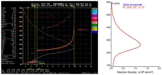
Figure 1.
Example (from (left) to (right)) of the ground-based HF (ionosonde) sounding recording with results of the ionogram processing and ionosonde-derived electron density profile Ne(h).
Our study also utilized COSMIC-2 electron density profiles as Level 2 data products provided by the UCAR COSMIC Data Analysis and Archive Center (CDAAC). These “ionPrf” files of ionospheric electron density profiles in netCDF format are publicly available via the CDAAC web portal [39]. Each “ionPrf” file contains information about altitude, latitude, and longitude of the RO tangent point and the corresponding electron density (Ne) value. CDAAC routinely processes RO observations as ionospheric EDP products using the Abel inversion technique from the ionospheric delay observations along the receiver–transmitter link. The retrieval technique for ionospheric electron density from GNSS RO measurements using the Abel inversion method is described in more detail by [40,41,42,43].
The data from all six COSMIC-2 satellites, marked further as C2E1 to C2E6, are available for both high-rate ionosonde campaign periods. Figure 2 shows the COSMIC-2 RO tangent point projections over the Ebre and El Arenosillo ionosondes’ area of operation in the October 2022 and March 2024 periods, illustrating the RO–ionosonde colocation geometry.
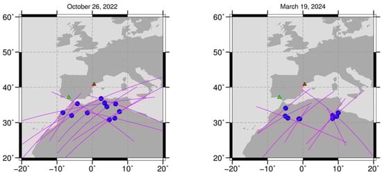
Figure 2.
COSMIC-2 RO observations with EDP tangent point projections (pink lines) for 26 October 2022 and 19 March 2024. The blue dots corresponded to the F2 layer peak locations derived from COSMIC-2 RO profiles. Red and green triangles pinpoint the Ebre and El Arenosillo ionosonde locations, respectively.
Our colocation criteria for the GNSS RO vs. ionosonde measurements are based on the spatial correlation factor of ionospheric plasma density variability. For the quiet-time midlatitude ionosphere, the correlation distance (correlation coefficient r > 0.70) can be considered as approximately 1500–3000 km in an east-west direction and 1000–1800 km in a north-south direction [44,45]. At low and equatorial latitudes, this correlation distance is shorter due to significantly larger temporal and spatial variability of the equatorial ionosphere, and it can be considered as 1000–1500 km in an east-west direction and 500–1000 km in a north-south direction [45]. It is also necessary to note that ionosonde soundings are not vertical incidences only; they detect echoes from the ionosphere within a wider angle of ~15° or more around the zenith, depending on the transmitting and receiving antenna patterns. This effect is also used for Directograms and Skymap Digisonde products, which estimate echo directions and plasma drift velocities [11].
Since the Ebre and El Arenosillo ionosondes are located close to southern midlatitudes, it is reasonable to select the maximal distance of ~1000 km (10°) as the criterion for a reliable colocation between the two independent ionospheric soundings from the ground and from an LEO. For selected COSMIC GNSS RO EDPs, the tangent point coordinates of the F2 peak point should be within a 10° radius of the ionosonde location, and a clear ionogram should be available within a ±5 min interval of the colocation time. With the most typical ionogram cadence of 15 min, the advantage of these high-rate ionosonde campaigns is that we can obtain more precise colocations in temporal domain.
Generally, the COSMIC-2 RO-derived peak parameters, peak density NmF2, and peak height hmF2 are in good agreement with the true values, similar to the ones derived from ground-based measurements. However, some RO profiles can be affected by uncertainties resulting from equatorial ionization anomaly impacts on RO soundings, because the Abel inversion retrieval method relies on a spherical symmetry assumption, which is not always valid at low latitudes [46,47,48,49]. To mitigate such issues, all COSMIC-2 RO electron density profiles were visually inspected in order to exclude potentially distorted or plasma-affected irregularities within the profiles. A couple of sample cases of COSMIC-2 RO electron density profiles, which were filtered out during quality control, are presented in Figure 3.
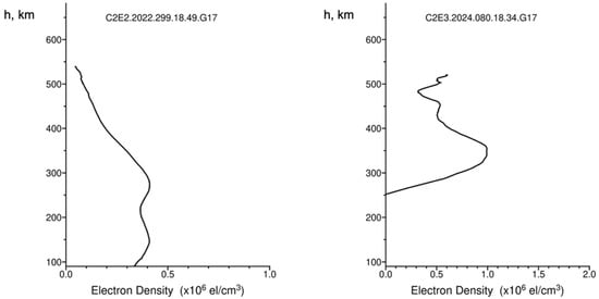
Figure 3.
Examples of COSMIC-2 RO electron density profiles distorted due to the impact of the equatorial ionization anomaly.
3. Results
For the set of colocations between COSMIC-2 RO and two ionosondes corresponding to the high-rate sounding campaigns in October 2022 and March 2024, we analyzed EDPs derived using two independent techniques with the data processing steps and selection criteria described in the previous sections. The analysis was performed not only by comparison of the F2 layer peak values derived from colocated EDPs, but also the shape of density distribution on the bottomside sections of the profiles from the observation lower limit to the F2 layer peak. In order to avoid Abel inversion related uncertainties in the absolute values of COSMIC-2 RO EDPs, each RO profile has been adjusted to match the unbiased F2 peak density values obtained from the colocated ionogram closest in time. This process was made separately for the Ebre and El Arenosillo ionosonde colocations. Such techniques are often used to calibrate EDPs derived from the incoherent scatter radar soundings when critical frequency measurements from a nearby ionosonde are applied to adjust the incoherent scatter radar plasma density profile [50,51].
As a result, we selected high-quality data products for the representative local time intervals corresponding to the geomagnetically quiet ionospheric conditions at moderate (October 2022) and high (March 2024) solar activity levels. While our result descriptions primarily focused on Ebre ionosonde observations, data from El Arenosillo was analyzed as well. Figure 4 illustrates several representative cases with the colocation events between COSMIC-2 RO and Ebre ionosonde EDPs in October 2022 (Day-Of-Year (DOY) 297-299). Figure 5 shows similar results, but for March 2024 (DOY 079-080). For each event, we combined the ionogram recordings and colocated EDP comparisons. The GNSS RO observations from LEO satellites do not provide redundant EDPs over the same locations daily, but as we mentioned before, the high-rate HF sounding campaigns provide opportunities to assess more colocation events due to the larger number of available ionograms within a time window. As a result, we can obtain precise RO–ionosonde EDP colocations for various local time conditions.
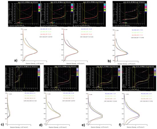
Figure 4.
(a–f) Representative examples of EDP colocation events between COSMIC-2 RO and the Ebre ionosonde combining ionogram recording and EDP comparisons for the October 2022 high-rate sounding campaign. The black line displays the COSMIC-2 RO EDP; the blue, green, and red lines show the time sequences of several ionosonde-derived EDPs. File names like “C2E1.2022.297.15.20.R01” mean COSMIC-2 satellite C2E1, year 2022, DOY (day-of-year) 297, time 15:20 UT, “R01”–tracking GLONASS satellite PRN 01. Ionosonde file names in plot captions share a similar structure.
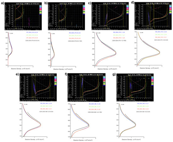
Figure 5.
The same as in Figure 4, but for the March 2024 high-rate sounding campaign (a–g).
In Figure 4a, we present the case of the closest-in-time colocation between two COSMIC-2 RO EDPs and time sequences of the Ebre ionosonde ionograms. Here, we have two COSMIC-2 occultations with a GLONASS R01 transmitter at ~15:20 UT on DOY 297, 2022, and with GPS G23 one minute later at ~15:21 UT that day. There are 1-min sequence ionosonde ionograms (15:19–15:22 UT, local daytime conditions) matching in time with these RO EDPs (three ionograms are placed on the top part of Figure 4a). The lower panel in Figure 4a displays COSMIC-2 RO EDPs (black lines) for these two cases overlaid on EDPs derived from the Ebre ionogram inversions (color lines, color corresponded to different sounding times). These results correspond to the afternoon ionosphere with well-developed daytime ionospheric layers. The COSMIC-2 RO and ionosonde profiles closely match near the F2 ionization peak by shape, and both techniques show the location of the F2 peak at an altitude of ~290 km. In the bottom section of all profiles, there are recognized E and F1 ionosphere layers, although some differences exist. The COSMIC-2 RO profiles show a more structured altitudinal density distribution within a 100–170 km range. These differences can be due to limitations in HF soundings, specifically in the E–F valley region where reflections from less dense upper layers cannot be obtained (e.g., [52]).
Other panels (b–d) in Figure 4 present cases of EDP colocations between COSMIC-2 RO and ionosonde for different local time conditions. The local time for the Ebre and El Arenosillo ionosonde locations is UTC + 01. Figure 4b corresponds to the pre-sunset hours (~17 LT) when both ionosonde and RO techniques show a decreasing of plasma density in the bottomside ionosphere and an absence of the developed E and F1 ionosphere layers. Figure 4c shows typical nighttime conditions: plasma density decreases across the entire profile while the F2 layer height increases. Figure 4d–f present cases of EDP colocations for daytime conditions of DOY 298–299, 2022. For the two cases (d–e), COSMIC-2 RO-derived profiles are reduced in the bottomside part of the ionosphere, which is below ~130 km, but still provide a reasonable performance around the F2 peak, with shape and density values close to the ionosonde-derived ones. The case (d) also shows some distortion in the topside part due to equatorial anomaly effects, which should be taken into account for future analyses.
Figure 5 shows representative examples of EDP colocation events that occurred during the second high-rate sounding campaign in March 2024 (DOY 079-080). For this period, we also have cases in different local times. Figure 5a,b illustrate nighttime conditions with typical low-density values and the F2 peak location above 300 km. For the case in Figure 5a, profiles are very well aligned, and for the case in Figure 5b, some differences exist in the bottomside area at the background of very low-density values. Figure 5c–f correspond to sunlit daytime conditions at different local times. Apart from pretty good agreement for these cases around the F2 layer, some discrepancies exist in the bottomside regions and relatively small differences are present near the F2 peak location. These differences can be explained in the same manner as for the October 2022 cases. We should note that the March 2024 period was characterized by high solar activity with ~170 SFU, and overall plasma density levels across profiles and near the F2 peaks are larger than those observed during the October 2022 campaign.
Figure 6 presents the EDP colocations between COSMIC-2 RO and the El Arenosillo ionosonde. Here, we selected representative daytime cases to investigate possible longitudinal differences between two ionosondes. The upper panel corresponds to the October 2022 high-rate sounding campaign and the bottom panel to the March 2024 campaign. The electron density profiles derived from GNSS RO and ionogram inversions show good agreement around the F2 layer peak, similar to the Ebre ionosonde findings. The bottomside discrepancies were more pronounced for the October 2022 cases. For the cases in March 2024, these differences in the EDP shape and in absolute values along profiles look less significant at the background of larger ionospheric plasma densities.
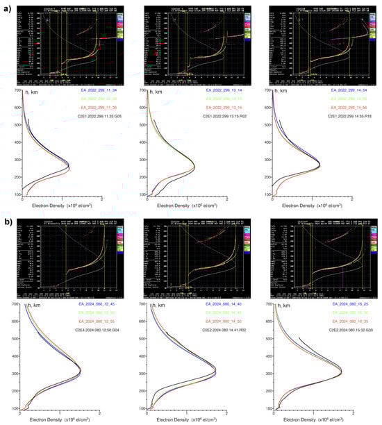
Figure 6.
Representative examples of EDP colocation events between COSMIC-2 RO and the El Arenosillo ionosonde combining ionogram recording and EDP comparisons for high-rate sounding campaigns on October 2022, panel (a), (daytime conditions, left to right 11:35, 13:15 and 14:55 UT hours) and March 2024, panel (b) (daytime conditions, left to right 12:50, 14:45 and 16:30 UT hours).
A comparative analysis of all these representative cases reveals generally good agreement in COSMIC-2 RO and ionosonde data in the bottomside parts of EDPs, whereas topside can exhibit significant variability. This is evidence of discrepancies in the topside part of these profiles. Thus, for practically all the analyzed cases, values of electron density in the topside part of the ionosonde-derived EDPs were lower than in RO profiles.
Since in the ionosonde-derived EDPs the topside part is obtained by model extrapolation fitting to the peak electron density value (no real data in the topside), COSMIC-2 experimental data can make an important contribution for investigating the topside ionosphere. Such combinations allow us to avoid fundamental limitations of the ground-based HF ionospheric soundings, which cannot measure plasma density above the F2 layer peak due to the lack of HF reflections from the less dense upper regions. At the same time, the unbiased measurements of plasma density in the bottomside ionosphere and at the F2 layer peak can mitigate GNSS RO retrieving uncertainties. Also, we should note that for RO missions operating in LEOs, there still exist limitations for the maximum altitudes of RO soundings pre-defined by the operational orbit (e.g., ~500–550 km for COSMIC-2 missions). The RO soundings from geostationary orbit potentially can solve this limitation as demonstrated by the GOES-based RO retrievals [53].
4. Discussion
Having precise in-time colocations between the Ebre and El Arenosillo ionosondes with COSMIC-2 RO EDPs allows us to combine these two different techniques of ionosphere probing in order to obtain a set of reference EDPs that cover an altitudinal range from 100 to 500–550 km. In such cases, the combined electron density profiles are constructed on the basis of only real observations without any artificial extrapolation. Both ionosonde and COSMIC-2 RO measurements provide already proven high-accuracy measurements within their areas of operation. These combined “best of the best” EDPs from ionosondes and RO are being calibrated to the unbiased values of the F2 layer peak plasma density and can serve as an analogy for incoherent scatter radar-derived “full profiles” as references for the altitudinal distribution of ionospheric plasma density. Such EDPs definitely can be used for ionospheric model validation.
Within this study framework, we examined this opportunity for the validation of the profile-based empirical International Reference Ionosphere (IRI) model. IRI is an empirical (data-based) model representing primary ionospheric parameters based on a long data record that exists from ground- and space-based observations of the Earth’s ionosphere. The core model describes monthly averages of electron density, electron temperature, ion temperature, and ion composition globally in the altitude range from 60 to 2000 km. The IRI simulates the ionospheric vertical electron density profile by dividing it into six sub-regions, including the topside, the F2 bottomside, and the F1 layer. The F2 layer peak serves as a main anchor point for the F2 region. This means that the electron densities in the topside and bottomside areas are normalized to the F2-peak electron density NmF2. The full vertical electron density profile is described by a set of mathematical expressions, each valid in a defined range of altitude [54]. These expressions are described in the following sections starting from the topside down to the D region. All densities are in el/m3, all frequencies are in MHz, and heights are in km [55,56].
Here, we used the most up-to-date version of the IRI model, IRI-2020, which was released in 2022 and is freely available for the research community (http://irimodel.org/). The main input parameters of the IRI model are location, time, sunspot number or solar radio flux, and magnetic Ap/Kp index. We used the URSI coefficients to specify the F2 layer peak parameters and actual sunspot number and solar radio flux indices. The foF2 STORM model option was turned off because this study deals with the quiet geomagnetic conditions. The “NeQuick topside” option was used for the topside electron density profile specification. For modeling hmF2, we used the default option of the Shubin-COSMIC model, which was based on hmF2 data derived from ionosonde and COSMIC-1 RO observations [57].
Figure 7 illustrates comparison of the IRI-2020 calculated EDPs with the reference profiles combined from ionosonde and COSMIC-2 RO measurements during the selected night, day, and evening hours for 24–26 October 2022 and 19–20 March 2024. It is important to note that IRI is a climatological model. It provides predictions of the monthly average values of ionospheric electron densities, e.g., in the form of EDPs for a selected location and conditions. These profiles could not reflect day-by-day variability of the ionosphere. For some cases, IRI can show that its profile shape is in excellent agreement with other observations, like in Figure 7a, or with some discrepancies near the F2 peak, like in Figure 7d. Also, reasonable agreement between updated IRI-2020 profiles and real observation data was found during the daytime; IRI tends to slightly underestimate density around the F2 peak. Also, the model overestimates density around the F2 peak during the night hours and in the topside ionosphere. Overall, these results are in good agreement with the incoherent radar—IRI comparisons presented in [58].
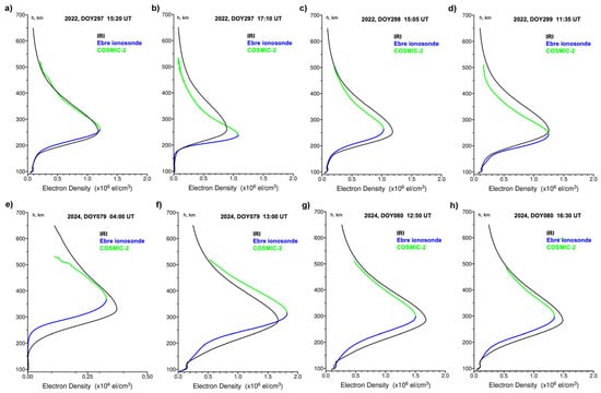
Figure 7.
Comparison of the electron density profiles derived from the IRI-2020 (black line) and the reference profiles combined from ionosonde (blue) and COSMIC-2 RO (green) measurements. Panels (a–d) corresponded to the October 2022 high-rate campaign observations and panels (e–h) corresponded to the March 2024 campaign.
In order to assess the performance of the IRI-2020 model in representing a real shape of electron density vertical distribution, we additionally compared our reference EDPs from the ionosonde and COSMIC-2 model with the IRI-2020 model simulation results generated with user-specified input of the F2 layer peak parameters (foF2 and hmF2). For this case, we used the real values of foF2 and hmF2 from our reference profiles to adjust the main anchor point in the IRI model formulation to the real parameters of the ionospheric peak.
Figure 8 presents the results of standard and adjusted versions of the IRI model outputs compared with the RO-ionosonde combined EDPs. We selected a few representative cases for daytime ionosphere conditions and overplotted the reference combined EDPs (indicated by bluegreen lines describing ionosonde and RO parts), standard IRI EDP output (black line), and adjusted IRI profiles with user-specified F2 layer peak parameters derived from the corresponding combined EDPs (red dots). Top and bottom panels in Figure 8 illustrate cases corresponding to the October 2022 and the March 2024 campaigns, respectively. The obtained results demonstrate clear differences in the EDPs’ shapes and peak values (up to 20% in density) in the model simulation outputs between the standard IRI and the corrected version with the real F2 layer peak values.
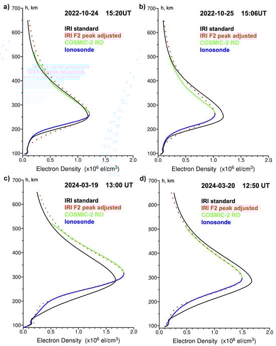
Figure 8.
Comparison of the IRI-2020 adjusted EDPs (red dots) with reference combined EDPs (blue-green line). The standard IRI output is shown as a black line. Panels (a,b) corresponded to the 24–25 October 2022 afternoon conditions and panels (c,d) corresponded to the 19–20 March 2024 noon hours.
The data–model discrepancies in the standard IRI outputs for the F2 peak values near the same local time on two consecutive days can result from the climatological nature of the model, driven by monthly averaged solar activity indices, which cannot reproduce accurately day-to-day ionospheric variability. When we adjusted the model ingesting the real observations even in single anchor points at the F2 layer peak, the absolute data–model differences became essentially smaller, especially around the main peak of ionospheric ionization. With this adjustment approach, we can better depict differences between observations and models in the bottomside ionosphere (E–F layers range), as well as in the topside ionosphere above the F2 layer peak up to ~500 km altitude, where we still have real observations. The biggest data–model discrepancies were found for the October 2022 moderate solar activity period. The model overestimated plasma density for the bottomside ionosphere by up to 45% (140–180 km altitudinal range). Above the F2 layer peak, the model also tended to overestimate observations by up to 15%. For the high solar activity (March 2024) and near noon hours, the data–model discrepancies with adjusted IRI were also mainly pronounced in the bottomside of the profile, but estimated differences did not exceed 10%, and the model tended to underestimate measurements there.
The obtained results demonstrate a significant discrepancy in most cases for the standard IRI model output both in absolute values of electron density and in altitudes. At the same time, we found pretty good agreement between the adjusted IRI profiles within an altitudinal range of ~±50 km around the F2 layer peak and the reference values, but some noticeable discrepancies exist in the topside and bottomside parts of the ionospheric plasma density vertical distributions. So, the IRI model still needs to be improved for a more precise electron density representation, and the combined electron density profiles derived from real observations by ground-based ionosondes and by satellite-based GNSS RO can contribute towards this important task.
5. Conclusions
By analyzing high-sampling-rate observations from the Ebre and El Arenosillo ionosonde stations with colocated COSMIC-2 RO measurements, we demonstrated how to create the combined ionospheric EDPs based solely on real high-quality observations from both the bottomside and topside parts of the ionosphere. Such combined EDPs can serve as an analogy for incoherent scatter radar-derived “full profiles”, providing a reference for the altitudinal distribution of ionospheric plasma density. These reference profiles offer a valuable data source for validating and further improving empirical ionospheric models.
Author Contributions
Conceptualization, I.C. and D.A.; methodology, I.C. and D.A.; software, I.Z.; validation, I.C., D.A. and I.Z.; formal analysis, I.C., D.A. and I.Z.; investigation, I.C., D.A., I.Z., D.H., V.d.P., V.N.-P., A.S. and I.G.; resources, D.H., V.d.P., V.N.-P., A.S. and I.G.; data curation, D.H., V.d.P., V.N.-P., A.S. and I.G.; writing—original draft preparation, I.C.; writing—review and editing, I.C., D.A. and I.Z.; visualization, I.Z., I.C. and D.A.; supervision, I.C.; project administration, I.C. and D.A.; funding acquisition, I.C. and D.A. All authors have read and agreed to the published version of the manuscript.
Funding
This research was funded by the PITHIA-NRF project. The PITHIA-NRF project has received funding from the European Union’s Horizon 2020 research and innovation program under grant agreement No. 101007599. This research was partially funded by the National Science Foundation (Grant 2054356) and the National Aeronautics and Space Administration (Grants C22K0658 and 80NSSC20K1733).
Institutional Review Board Statement
Not applicable.
Informed Consent Statement
Not applicable.
Data Availability Statement
We acknowledge the COSMIC CDAAC for providing RO electron density profiles from the COSMIC-2 mission (UCAR COSMIC Program, https://doi.org/10.5065/t353-c093). Raw ionograms from the Ebre and El Arenosillo digisondes are available through the GIRO database (http://giro.uml.edu/, accessed on 25 June 2025) and were scaled using the SAO Explorer tool (https://ulcar.uml.edu/SAO-X/SAO-X.html, accessed on 25 June 2025).
Conflicts of Interest
The authors declare no conflicts of interest.
Abbreviations
The following abbreviations are used in this manuscript:
| RO | Radio Occultation |
| COSMIC | Constellation Observing System for Meteorology, Ionosphere, and Climate |
| GNSS | Global Navigation Satellite System |
| EDP | Electron density profile |
| IRI | International Reference Ionosphere |
References
- Reinisch, B. Ionosonde. In The Upper Atmosphere; Dieminger, W., Hartmann, G.K., Leitinger, R., Eds.; Springer: Berlin/Heidelberg, Germany, 1996; pp. 370–381. [Google Scholar]
- Huang, X.; Reinisch, B.W. Vertical electron density profiles from the digisonde network. Adv. Space Res. 1996, 18, 121–129. [Google Scholar] [CrossRef]
- Farley, D.T. Incoherent scatter power measurements; a comparison of various techniques. Radio Sci. 1969, 4, 139–142. [Google Scholar] [CrossRef]
- Jakowski, N.; Leitinger, R.; Angling, M. Radio occultation techniques for probing the ionosphere. Ann. Geophys. 2004, 47, 1049–1066. [Google Scholar] [CrossRef]
- Tsai, L.C.; Liu, C.H.T.; Tsai, W.H.; Liu, C.H.T. Tomographic imaging of the ionosphere using the GPS/MET and NNSS data. J. Atmos. Sol.-Terr. Phys. 2002, 64, 2003–2011. [Google Scholar] [CrossRef]
- Appleton, E.V.; Ingram, L.J. Magnetic storms and upper atmosphere ionisation. Nature 1935, 136, 548–549. [Google Scholar] [CrossRef]
- Booker, H.G.; Wells, H.W. Scattering of radio waves by the F-region of the ionosphere. Terr. Magn. Atmos. Electr. 1938, 43, 249–256. [Google Scholar] [CrossRef]
- Ratcliffe, J.A. A quick method for analysing ionospheric records. J. Geophys. Res. 1951, 56, 463–485. [Google Scholar] [CrossRef]
- Yonezawa, T.; Arima, Y. On the seasonal and non-seasonal annual variations and the semi-annual variation in the noon and midnight electron densities of the F2 layer in middle latitudes. J. Radio Res. Labs 1959, 6, 293–309. [Google Scholar]
- Reinisch, B.W. Modern Ionosondes. In Modern Ionospheric Science; Kohl, H., Ruster, R., Schlegel, K., Eds.; European Geophysical Society: Katlenburg-Lindau, Germany, 1996; pp. 440–458. [Google Scholar]
- Galkin, I.A. Ionospheric Imaging with Ionosondes: Historical Perspective and Prospective Insight. In 100 Years of the International Union of Radio Science; Wilkinson, P., Cannon, P.S., Stone, W.R., Eds.; URSI Press: Gent, Belgium, 2021; Chapter 29, Section 2; pp. 520–528. ISBN 9789463968034. [Google Scholar]
- Piggott, W.R.; Rawer, K. URSI Handbook of Ionogram Interpretation and Reduction; Piggott, W.R., Rawer, K., Eds.; Report UAG 23A; World Data Center A for Solar-Terrestrial Physics, NOAA: Boulder, CO, USA, 1978. Available online: https://repository.library.noaa.gov/view/noaa/10404/noaa_10404_DS1.pdf (accessed on 26 June 2025).
- Titheridge, J.E. The real height analysis of ionograms: A generalized formulation. Radio Sci. 1988, 23, 831–849. [Google Scholar] [CrossRef]
- Reinisch, B.W.; Huang, X. Automatic calculation of electron density profiles from digital ionograms: 3. Processing of bottomside ionograms. Radio Sci. 1983, 18, 477–492. [Google Scholar] [CrossRef]
- Scotto, C. Electron density profile calculation technique for Autoscala ionogram analysis. Adv. Space Res. 2009, 44, 756–766. [Google Scholar] [CrossRef]
- Reinisch, B.W.; Galkin, I.A.; Khmyrov, G.M.; Kozlov, A.V.; Bibl, K.; Lisysyan, I.A.; Cheney, G.P.; Huang, X.; Kitrosser, D.F.; Paznukhov, V.V.; et al. New Digisonde for research and monitoring applications. Radio Sci. 2009, 44, RS0A24. [Google Scholar] [CrossRef]
- DPS4D Specification. Digisonde-4D System Manual, Version 1.2.6. 2020. Available online: https://digisonde.com/pdf/Digisonde4DManual_LDI-web.pdf (accessed on 25 June 2025).
- Hajj, G.A.; Romans, L.J. Ionospheric electron density profiles obtained with the Global Positioning System: Results from the GPS/MET experiment. Radio Sci. 1998, 33, 175–190. [Google Scholar] [CrossRef]
- Schreiner, W.S.; Sokolovskiy, S.V.; Rocken, C.; Hunt, D.C. Analysis and validation of GPS/MET radio occultation data in the ionosphere. Radio Sci. 1999, 34, 949–966. [Google Scholar] [CrossRef]
- Rocken, C.; Kuo, Y.H.; Scheriner, W.S.; Hunt, D.; Sokolovskiy, S.; Mccormick, C. COSMIC system description. Terr. Atmos. Ocean. Sci. 2000, 12, 119–138. [Google Scholar] [CrossRef]
- Anthes, R.A.; Bernhardt, P.A.; Chen, Y.; Cucurull, L.; Dymond, K.F.; Ector, D.; Healy, S.B.; Ho, S.-P.; Hunt, D.C.; Kuo, Y.; et al. The COSMIC/FORMOSAT-3 mission: Early results. Bull. Am. Meteorol. Soc. 2008, 89, 313–333. [Google Scholar] [CrossRef]
- Anthes, R.A. Exploring Earth’s atmosphere with radio occultation: Contributions to weather, climate and space weather. Atmos. Meas. Tech. 2011, 4, 1077–1103. [Google Scholar] [CrossRef]
- Lei, J.; Syndergaard, S.; Burns, A.G.; Solomon, S.C.; Wang, W.; Zeng, Z.; Roble, R.G.; Wu, Q.; Kuo, Y.-H.; Holt, J.M.; et al. Comparison of COSMIC ionospheric measurements with ground-based observations and model predictions: Preliminary results. J. Geophys. Res. Space Phys. 2007, 112, A07308. [Google Scholar] [CrossRef]
- Kelley, M.C.; Wong, V.K.; Aponte, N.; Coker, C.; Mannucci, A.J.; Komjathy, A. Comparison of COSMIC occultation-based electron density profiles and TIP observations with Arecibo incoherent scatter radar data. Radio Sci. 2009, 44, RS4011. [Google Scholar] [CrossRef]
- Chu, Y.H.; Su, C.L.; Ko, H.T. A global survey of COSMIC ionospheric peak electron density and its height: A comparison with ground-based ionosonde measurements. Adv. Space Res. 2010, 46, 431–439. [Google Scholar] [CrossRef]
- Krankowski, A.; Zakharenkova, I.; Krypiak-Gregorczyk, A.; Shagimuratov, I.; Wielgosz, P. Ionospheric electron density observed by FORMOSAT-3/COSMIC over the European region and validated by ionosonde data. J. Geod. 2011, 85, 949–964. [Google Scholar] [CrossRef]
- Cherniak, I.V.; Zakharenkova, I.E. Validation of FORMOSAT-3/COSMIC radio occultation electron density profiles by incoherent scatter radar data. Adv. Space Res. 2014, 53, 1304–1312. [Google Scholar] [CrossRef]
- Habarulema, J.B.; Katamzi, Z.T.; Yizengaw, E. A simultaneous study of ionospheric parameters derived from FORMOSAT-3/COSMIC, GRACE, and CHAMP missions over middle, low, and equatorial latitudes: Comparison with ionosonde data. J. Geophys. Res. Space Phys. 2014, 119, 7732–7744. [Google Scholar] [CrossRef]
- McNamara, L.F.; Thompson, D.C. Validation of COSMIC values of foF2 and M(3000)F2 using ground-based ionosondes. Adv. Space Res. 2015, 55, 163–169. [Google Scholar] [CrossRef]
- Pedatella, N.M.; Yue, X.; Schreiner, W.S. An improved inversion for FORMOSAT-3/COSMIC ionosphere electron density profiles. J. Geophys. Res. Space Phys. 2015, 120, 8942–8953. [Google Scholar] [CrossRef]
- Yue, X.; Schreiner, W.S.; Pedatella, N.; Anthes, R.A.; Mannucci, A.J.; Straus, P.R.; Liu, J.-Y. Space weather observations by GNSS radio occultation: From FORMOSAT-3/COSMIC to FORMOSAT-7/COSMIC-2. Space Weather. 2014, 12, 616–621. [Google Scholar] [CrossRef]
- Schreiner, W.S.; Weiss, J.P.; Anthes, R.A.; Braun, J.; Chu, V.; Fong, J.; Hunt, D.; Kuo, Y.-H.; Meehan, T.; Serafino, W.; et al. COSMIC-2 radio occultation constellation: First results. Geophys. Res. Lett. 2020, 47, e2019GL086841. [Google Scholar] [CrossRef]
- Weiss, J.P.; Schreiner, W.S.; Braun, J.J.; Xia-Serafino, W.; Huang, C.Y. COSMIC-2 Mission Summary at Three Years in Orbit. Atmosphere 2022, 13, 1409. [Google Scholar] [CrossRef]
- Cherniak, I.; Zakharenkova, I.; Braun, J.; Wu, Q.; Pedatella, N.; Schreiner, W.; Weiss, J.-P.; Hunt, D. Accuracy assessment of the quiet-time ionospheric F2 peak parameters as derived from COSMIC-2 multi-GNSS radio occultation measurements. J. Space Weather. Space Clim. 2021, 11, 18. [Google Scholar] [CrossRef]
- Chen, C.F.; Reinisch, B.W.; Scali, J.L.; Huang, X.; Gamache, R.R.; Buonsanto, M.J.; Ward, B.D. The accuracy of ionogram-derived N(h) profiles. Adv. Space Res. 1994, 14, 43–46. [Google Scholar] [CrossRef]
- Dandenault, P.B.; Dao, E.; Kaeppler, S.R.; Miller, E.S. An estimation of human-error contributions to historical ionospheric data. Earth Space Sci. 2020, 7, e2020EA001123. [Google Scholar] [CrossRef]
- Reinisch, B.W.; Galkin, I.A. Global ionospheric radio observatory (GIRO). Earth Planets Space 2011, 63, 377–381. [Google Scholar] [CrossRef]
- Reinisch, B.W.; Huang, X. Deducing topside profiles and total electron content from bottomside ionograms. Adv. Space Res. 2001, 27, 23–30. [Google Scholar] [CrossRef]
- UCAR COSMIC Program. COSMIC-2 Data Products [IonPrf Dataset]; UCAR/NCAR—COSMIC: Boulder, CO, USA, 2019. [Google Scholar] [CrossRef]
- Syndergaard, S.; Schreiner, W.S.; Rocken, C.; Hunt, D.C.; Dymond, K.F. Preparing for COSMIC: Inversion and analysis of iono- spheric data products. In Atmosphere and Climate: Studies by Occultation Methods; Foelsche, U., Kirchengast, G., Steiner, A.K., Eds.; Springer: New York, NY, USA, 2006; pp. 137–146. [Google Scholar]
- Tsai, L.C.; Tsai, W.H.; Schreiner, W.S.; Berkey, F.T.; Liu, J.Y. Comparisons of GPS/MET retrieved ionospheric electron density and ground based ionosonde data. Earth Planets Space 2001, 53, 193–205. [Google Scholar] [CrossRef]
- Chou, M.Y.; Lin, C.C.H.; Tsai, H.F.; Lin, C.Y. Ionospheric electron density inversion for global navigation satellite systems radio occultation using aided Abel inversions. J. Geophys. Res. Space Phys. 2017, 122, 1386. [Google Scholar] [CrossRef]
- Healy, S.B.; Haase, J.; Lesne, O. Abel Transform Inversion of Radio Occultation Measurements Made with a Receiver inside the Earth’s Atmosphere. Ann. Geophys. 2022, 20, 1253–1256. [Google Scholar] [CrossRef]
- Rush, C.M.; Edwards, W.R. An automated mapping technique for representing the hourly behavior of the ionosphere. Radio Sci. 1976, 11, 931–937. [Google Scholar] [CrossRef]
- Klobuchar, J.A.; Kunches, J.M. Eye on the ionosphere: The spatial variability of ionospheric range delay. GPS Solut. 2000, 3, 70–74. [Google Scholar] [CrossRef]
- Yue, X.; Schreiner, W.S.; Lei, J.; Sokolovskiy, S.V.; Rocken, C.; Hunt, D.C.; Kuo, Y.H. Error analysis of Abel retrieved electron density profiles from radio occultation measurements. Ann. Geophys. 2010, 28, 217–222. [Google Scholar] [CrossRef]
- Yue, X.; Schreiner, W.S.; Rocken, C.; Kuo, Y.H.; Lei, J. Artificial ionospheric wave number 4 structure below the F2 region due to the Abel retrieval of radio occultation measurements. GPS Solut. 2012, 16, 1–7. [Google Scholar] [CrossRef]
- Mannucci, A.J.; Ao, C.O.; Pi, X.; Iijima, B.A. The impact of large scale ionospheric structure on radio occultation retrievals. Atmos. Meas. Tech. 2011, 4, 2837–2850. [Google Scholar] [CrossRef]
- Kulikov, I.; Mannucci, A.J.; Pi, X.; Raymond, C.; Hajj, G.A. Electron density retrieval from occulting GNSS signals using a gradient-aided inversion technique. Adv. Space Res. 2011, 47, 289–295. [Google Scholar] [CrossRef]
- Evans, J.V. Theory and practice of ionosphere study by Thomson scatter radar. Proc. IEEE 1969, 57, 496–530. [Google Scholar] [CrossRef]
- Sato, T.; Ito, A.; Oliver, W.L.; Fukao, S.; Tsuda, T.; Kato, S.; Kimura, I. Ionospheric incoherent scatter measurements with the middle and upper atmosphere radar: Techniques and capability. Radio Sci. 1989, 24, 85–98. [Google Scholar] [CrossRef]
- Lobb, R.J.; Titheridge, J.E. The valley problem in bottomside ionogram analysis. J. Atmos. Sol.-Terr. Phys. 1977, 39, 35–42. [Google Scholar] [CrossRef]
- Zakharenkova, I.; Cherniak, I.; Gleason, S.; Hunt, D.; Freesland, D.; Krimchansky, A.; McCorkel, J.; Ramsey, G. Ionospheric Electron Density Profiles Retrievals from GPS Observations Onboard Geostationary GOES Satellites: First Results and Validation. J. Space Weather. Space Clim. 2023, 13, 23. [Google Scholar] [CrossRef]
- Bilitza, D.; Truhlik, V.; Yoshihara, O.; Moldwin, M.B. Development and Improvement of the International Reference Ionosphere with special emphasis on the topside and extension to the plasmasphere. Ann. Geophys. 2024, 67, SA443. [Google Scholar] [CrossRef]
- Bilitza, D.; Pezzopane, M.; Truhlik, V.; Altadill, D.; Reinisch, B.W.; Pignalberi, A. The International Reference Ionosphere Model: A Review and Description of an Ionospheric Benchmark. Rev. Geophys. 2022, 60, e2022RG000792. [Google Scholar] [CrossRef]
- Bilitza, D. IRI the International Standard for the Ionosphere. Adv. Radio Sci. 2018, 16, 1–11. [Google Scholar] [CrossRef]
- Shubin, V.N. Global median model of the F2-layer peak height based on ionospheric radio-occultation and ground based Digisonde observations. Adv. Space Res. 2015, 56, 916–928. [Google Scholar] [CrossRef]
- Cherniak, I.; Dzubanov, D.; Zakharenkova, I.E. Accuracy of IRI profiles of ionospheric density and temperatures derived from comparisons to Kharkov incoherent scatter radar measurements. Adv. Space Res. 2011, 51, 639–646. [Google Scholar] [CrossRef]
Disclaimer/Publisher’s Note: The statements, opinions and data contained in all publications are solely those of the individual author(s) and contributor(s) and not of MDPI and/or the editor(s). MDPI and/or the editor(s) disclaim responsibility for any injury to people or property resulting from any ideas, methods, instructions or products referred to in the content. |
© 2025 by the authors. Licensee MDPI, Basel, Switzerland. This article is an open access article distributed under the terms and conditions of the Creative Commons Attribution (CC BY) license (https://creativecommons.org/licenses/by/4.0/).