Research on Air Temperature Inversion Method Based on Land Surface Temperature of Different Land Surface Cover

Abstract

This study explores a method for deriving air temperature (AT) from land surface temperature (LST) based on different urban land-use types, aiming to address the accuracy of urban heat island (UHI) effect measurements. Using Wuhan as a case study, the research integrates remote sensing data with ground meteorological observations to develop various models, analyze their accuracy and applicability, and generate LST and AT maps to validate model reliability. The results indicate that when establishing the LST–AT relationship, polynomial regression performs best for water bodies (R² = 0.905), while random forest yields the highest R² for built-up areas, cropland, and vegetation at 0.942, 0.953, and 0.924, respectively. Due to the characteristics of the algorithms, it is recommended to prioritize random forest for prediction when the sample range covers the observed data range and to use BP neural networks when it does not. The generated maps reveal that in summer, using LST significantly overestimates UHI intensity in the study area, while differences between UHI intensities in winter are negligible. In resource-constrained scenarios, LST can be directly used to assess the UHI effect.

1. Introduction

The urban heat island (UHI) effect leads to increased energy consumption and greenhouse gas emissions [1,2], negatively impacting urban air quality and raising the frequency of extreme weather events [3]. Therefore, efficiently measuring UHI and assessing its severity is critical for addressing the environmental changes brought by urbanization.

Methods for measuring the UHI effect primarily fall into two categories: land surface temperature (LST) and air temperature (AT) [4]. The surface urban heat island (SUHI) effect is assessed using remote sensing to measure LST, providing high-resolution urban thermal environment imagery suitable for large-scale monitoring. However, LST measurements are influenced by surface characteristics and weather conditions and reflect LST rather than actual AT. In contrast, the atmospheric urban heat island (AUHI) effect is evaluated by measuring near-surface AT at meteorological stations, which directly reflects temperature differences perceived by humans and offers good temporal continuity. However, its spatial resolution is limited, as it depends on the distribution of meteorological stations, making it challenging to provide continuous urban thermal environment information [5]. For these reasons, researchers have attempted to derive AT from LST to better understand and monitor the UHI effect on a larger spatial scale.

Some scholars have used physical meteorological parameters to establish the relationship between LST and AT [6,7,8,9,10]. For instance, Majkowska et al. developed linear and nonlinear regression models to estimate AT in Poznań [11]. Azevedo et al. estimated the temporal variation of the urban heat island index using differences in sensible heat flux, wind, and urban length scales [12]. Oke et al. proposed a diurnal UHI model based on weather factors, incorporating cloud fraction and type, as well as the −1/2 power of wind speed [13]. Theeuwes et al. analyzed meteorological station data from Western Europe, solar radiation, diurnal temperature range, wind speed, and vertical temperature gradients to determine UHI intensity by observing screen-level temperatures, solar radiation, and rural 10 m wind speeds [14]. Although these studies have demonstrated accurate conversions between LST and AT, they often require specific information on wind speed and direction, which can only be measured point-by-point, making it difficult to obtain large-scale AT data [15,16].

Other researchers have established statistical models to estimate AT from LST. For example, Pradhan et al. proposed an empirical equation for calculating AT from remotely sensed LST data in the Himalayan region [17]. Hassaballa et al. compared the correlation between LST estimated via the split-window algorithm and observed AT [18]. Mutiibwa et al. evaluated the applicability and limitations of using LST as a substitute or input variable to predict AT in complex mountainous terrain [19]. He et al. developed a method for predicting AT in glacial regions using random forest models and ERA5 data [20]. Ye et al. incorporated vegetation index, LST, and slope as factors into long short-term memory (LSTM) neural networks, predicting AT at unobserved locations based on meteorological station data [21]. However, these studies often rely on a single model, lacking comparisons between different models. Additionally, the relationship between LST and AT is influenced by factors such as land cover and land-use (LCLU) types, urban structure, and regional climatic conditions [22,23]. Different LCLU types correspond to varying thermal environments, necessitating a more precise understanding of the LST–AT relationship. Figure 1 shows the workflow diagram of this study.

Thus, the objectives of this study are as follows:

• To establish relationships between LST and AT for different land-use types and evaluate the applicability of various modeling methods.
• To integrate the derived relationships with LST imagery to generate spatially continuous AT maps.

2. Materials and Methods

2.1. Study Area

Wuhan, located between latitudes 29°58′–31°22′ N and longitudes 113°41′–115°05′ E, is the capital city of Hubei Province, China (Figure 2). Since the reform and opening-up policy, Wuhan has experienced rapid population growth, a high urbanization rate, and significant land-use changes [24]. By the end of 2023, the city had a permanent population of 13.774 million, and an urbanization rate of 84.66%. Wuhan features a humid subtropical monsoon climate characterized by hot summers and cold winters (Figure 3 and Figure 4). Summer spans from June to August, and winter lasts from December to February. The monthly average temperature in summer is between 25 and 30 °C, while the monthly average temperature in winter is between 4 and 7 °C. The annual average relative humidity is 76%, marking it as a typical hot-summer, cold-winter climate zone. Given these climatic conditions, it is necessary to analyze the urban heat island (UHI) effect separately for summer and winter seasons to improve the thermal environment.

2.2. Data Sources

The land-use data were obtained from the Annual China Land Cover Dataset (CLCD) published by Yang Jie et al. This dataset integrates data from the China Land-Use/Cover Dataset (CLUDs) and classifies land use into nine categories: farmland, forest, shrubland, grassland, water, ice/snow, barren land, impervious surfaces, and wetlands [25]. Wuhan is a highly developed provincial capital, where there are no ice and snow areas, and the proportion of wetlands and bare land is extremely low. Forests, shrubs, and grasslands show consistency in their impact on the thermal environment. Therefore, this study performed a reclassification based on this foundation and conducted statistics on the remote sensing data using Envi software (version 4.2). Ice and snow, as well as wetland types without corresponding data, were removed, and the bare land type, which accounts for less than 0.1%, was merged into the built-up area. The three categories of forest, shrub, and grassland were combined into one category (vegetation), as shown in

Table 1. Land-Use Classification Table.

Original Type	Reclassified Type
farmland	farmland
forest	vegetation
shrubland	vegetation
grassland	vegetation
water	water
ice/snow	no corresponding area
barren land	build
impervious surfaces	build
wetlands	no corresponding area

.

The satellite remote sensing data were sourced from the Landsat-7 ETM+ and Landsat-8 OLI datasets provided by the United States Geological Survey (USGS), with a spatial resolution of 30 m × 30 m. Each downloaded Landsat dataset includes three adjacent paths (Path/Row: 122/39, 123/38, and 123/39). The data were collected at approximately 11:00 a.m. Additionally, MODIS data from NASA, with a spatial resolution of 1 km × 1 km, were utilized. To ensure data quality, only images with less than 5% cloud cover from 2013 to 2019 were selected [26]. The information on the remote sensing images is shown in

Table 2. Remote sensing data list (Imaging time is in Beijing time).

Data Number	Acquisition Date	Imaging Time	Cloud Coverage
1	11 October 2013	10:52	0%
2	28 November 2013	10:52	0%
3	1 December 2014	10:54	2%
4	29 July 2015	10:56	0%
5	17 October 2015	10:56	0%
6	6 December 2016	10:58	0%
7	13 April 2017	10:58	3%
8	29 April 2017	10:58	0%
9	26 November 2018	10:52	0%
10	25 August 2019	10:43	0%

.

Meteorological data used for model training included hourly air temperature records from various stations in Wuhan, sourced from the Hubei Meteorological Bureau. Although the distribution of meteorological stations within the study area is relatively scattered, the model only requires data collection for training rather than directly using meteorological station data to evaluate the thermal environment; therefore, the impact is minimal. These stations cover most land-use types, with their geographic distribution shown in the corresponding figure. Meteorological data for error analysis were sourced from the U.S. National Weather Service (NWS), which collaborates with the World Meteorological Organization (WMO) to provide global meteorological data, including temperature, precipitation, and wind speed.

2.3. Research Methods

2.3.1. Land Surface Temperature Retrieval

To enhance the correlation between surface temperature and air temperature, this study utilizes high-accuracy Landsat series data. Starting in January 2024, NASA will discontinue the provision of atmospheric transmittance queries and will instead provide processed data directly. Consequently, the previously commonly used single-window algorithm is no longer applicable. By consulting the guidelines from the U.S. Geological Survey regarding the processing of Landsat Level-2 scientific products, which includes specifications for the scaling factors and offsets for each band, the following algorithm can be used to scale the ST-B6 (thermal infrared) band in remote sensing images:

$$Ts=DN\ast 0.00341802+149-273.15$$

(1)

where $Ts$ represents the surface temperature in degrees Celsius, and $DN$ denotes the band digital number.

However, due to sensor malfunctions on the Landsat 7 satellite, some remote sensing images have missing data. There are four locations where missing images overlap with study sites, so this research employs MODIS series images as supplements [27].

First, read the remote sensing data in ENVI (version 4.2), obtaining the thermal infrared dataset’s bands 31 and 32. The radiance calibration coefficients for each band are extracted and scaled using the following formulas:

$$B_{31}=0.00084002\ast ({DN}_{31}-1577.334)$$

(2)

$$B_{32}=0.00072970\ast ({DN}_{32}-1658.22)$$

(3)

where $B_i$ is the radiance of each band, and $DN$ is the displayed value of the band. Then, the reflectance dataset included in the remote sensing data is located, selecting spatial and spectral subsets near Wuhan, and performing geometric correction on the reflectance data. After the correction is completed, the split-window algorithm’s calculations are performed. The formula is as follows:

$$Ts=A_0+A_1\ast T_{31}-A_2\ast T_{32}$$

(4)

In this equation, $Ts$ refers to the surface temperature, while $T_{31}$ and $T_{32}$ are the brightness temperatures of MODIS’s 31st and 32nd bands, respectively. The parameters $A_0$, $A_1$, and $A_2$ of the split-window algorithm are defined as follows:

$$\begin{gathered} A_0=\left[D_{32}\right(1-C_{31}-D_{31})/(D_{31}{C}_{31}-D_{31}{C}_{32}\left)\right]a_{31}-\left[D_{31}\right(1 \\ -C_{32}-D_{32})/(D_{32}{C}_{31}-D_{31}{C}_{32}\left)\right]a_{32} \end{gathered}$$

(5)

$$\begin{gathered} A_1=1+D_{31}/(D_{31}{C}_{31}-D_{31}{C}_{32})+\left[D_{32}\right(1-C_{31} \\ -D_{31})/(D_{32}{C}_{31}-D_{31}{C}_{32}\left)\right]b_{32} \end{gathered}$$

(6)

$$\begin{gathered} A_2=D_{31}/(D_{32}{C}_{31}-D_{31}{C}_{32})+\left[D_{31}\right(1-C_{32}-D_{32})/(D_{32}{C}_{31} \\ -D_{31}{C}_{32}\left)\right]b_{32} \end{gathered}$$

(7)

Intermediate parameters in these formulas are defined as follows:

$$C_i={\mathsf{Ɛ}}_i\ast {\tau }_i\left(\mathsf{ɵ}\right)$$

(8)

$$D_i=[1-{\tau }_i(\mathsf{ɵ}\left)\right][1+(1-{\mathsf{Ɛ}}_i\left){\tau }_i\right(\mathsf{ɵ}\left)\right]$$

(9)

where ${\tau }_i\left(\mathsf{ɵ}\right)$ is the atmospheric transmittance at angle ɵ, and ${\mathsf{Ɛ}}_i$ is the surface emissivity for band i. Additional values for atmospheric transmittance, surface emissivity, and brightness temperature are required to perform surface temperature retrieval.

The atmospheric transmittance ${\tau }_i\left(\mathsf{ɵ}\right)$ is a fundamental parameter for calculating surface temperature, indicating the ability of the atmosphere to transmit electromagnetic waves (such as light, infrared radiation, etc.). It represents the proportion of incident radiation energy that can pass through the atmosphere to reach the surface or a specific level, typically calculated based on atmospheric water vapor content. In this study, MODIS bands 2 and 19 are used to retrieve atmospheric moisture content, which is then used to obtain atmospheric transmittance. The atmospheric moisture content of any pixel in the MODIS image can be calculated using the following formula:

$$w_i={({\displaystyle \frac{\left[\alpha -\ln \left(\frac{{\rho }_{19}}{{\rho }_2}\right)\right]}{\beta }})}^2$$

(10)

Here, $w_i$ is the atmospheric moisture content (g/cm²), while $\alpha$ and $\beta$ are constants set at 0.02 and 0.6321, respectively. ${\rho }_2$ and ${\rho }_{19}$ are the ground reflectance values for bands 2 and 19. The simulated equations are utilized as follows:

$${\tau }_{31}\left(\mathrm{ɵ}\right)=2.89798-1.88366\ast \mathrm{e}\mathrm{x}\mathrm{p}\left({\displaystyle \frac{w_{31}}{21.22704}}\right)$$

(11)

$${\tau }_{32}\left(\mathrm{ɵ}\right)=-3.59289-4.60414\ast \mathrm{e}\mathrm{x}\mathrm{p}\left({\displaystyle \frac{w_{32}}{32.70639}}\right)$$

(12)

Thus, atmospheric transmittance can be obtained.

Surface emissivity refers to the ability of surface materials to emit radiation relative to a black body (an ideal radiator) at the same temperature. Its value typically ranges between 0 and 1, where 1 signifies perfect radiation (black body) and 0 signifies no radiation. Surface emissivity depends on factors such as material, surface roughness, temperature, and wavelength, meaning it is influenced by the land-use status of the region. The study area is divided into three categories: water surface, urban areas, and natural surfaces. A mixed pixel decomposition method is utilized to calculate the emissivity for natural surfaces and urban areas based on vegetation coverage, which is calculated as follows:

First, the Normalized Difference Vegetation Index (NDVI) must be obtained. This is a widely used remote sensing metric primarily used to assess the health, density, and growth of vegetation coverage. NDVI quantifies greenness and biomass by combining data from red and near-infrared bands. NDVI values typically range from −1 to 1, with higher values indicating healthier and denser vegetation. Values between 0 and 1 represent areas with sparse or dense vegetation. Values close to 0 typically indicate no vegetation and may include bare soil, water bodies, or urbanized areas, while negative values indicate non-vegetative surface features such as water bodies, clouds, snow, or ice. The calculation is as follows:

$$NDVI=(NIR-RED)/(NIR+RED)$$

(13)

where $NIR$ is the reflectance value for the near-infrared band, and $RED$ is the reflectance value for the red band; both are obtainable from remote sensing data. After obtaining the NDVI, the vegetation coverage ($P_v$) can be calculated. This value measures the coverage rate of surface vegetation, with higher values indicating more abundant vegetation. The calculation is as follows:

$$P_v=(NDVI-{NDVI}_{min})/({NDVI}_{max}-{NDVI}_{min})$$

(14)

where ${NDVI}_{min}$ represents the minimum NDVI within the study area, generally indicating bare land or built-up areas, and ${NDVI}_{max}$ represents the maximum NDVI within the study area, usually indicating dense vegetation. After that, surface emissivity ${\mathsf{Ɛ}}_i$ can be obtained. For vegetated and arable areas, the following formula applies:

$${\mathsf{Ɛ}}_i=-0.0461{P_v}^2+0.0614P_v+0.9625$$

(15)

For built-up areas, the formula is

$${\mathsf{Ɛ}}_i=-0.0671{P_v}^2+0.086P_v+0.9589$$

(16)

For water bodies, since their radiative properties are almost equivalent to a black body, constants are directly used: ε₃₁ = 0.996, ε₃₂ = 0.992.

The radiance temperature must be calculated using the Planck function, which describes the spectral distribution of black-body radiation, expressing the relationship between the radiation intensity emitted by a black body at a specific temperature and wavelength. The Planck function can explain how the radiation intensity emitted by an object varies across different wavelengths; in this study, it takes the following forms:

$$T_{31}=1304.413871/ln(1+729.541636/{DN}_{31})$$

(17)

$$T_{32}=1196.978785/ln(1+474.684780/{DN}_{32})$$

(18)

At this point, all parameters in Formula (4) have been obtained. By substituting these parameters and handling any outliers, the surface temperature can be derived.

To account for errors arising from the mixed use of different remote sensing data, we also employ the method developed by Huanfeng Shen et al. [28]. to calibrate remotely sensed images of varying resolutions. The principle of this method is that the error values for different-resolution images at any given location are the same. Before calibration, it is essential that all data from different sensors is re-projected and sampled onto a common spatial grid. Thus, we defined a common coordinate system (WGS1984) for both Landsat and MODIS data within ArcGIS. The equation for calibration is as follows:

$$F\left(i,t_2\right)=F\left(i,t_1\right)+M\left(i,t_2\right)-M\left(i,t_1\right)$$

(19)

where $F\left(i,t_2\right)$ is the temperature corresponding to the missing moment of the high-resolution satellite, $F\left(i,t_1\right)$ is the known temperature at another moment, and $M\left(i,t_2\right)$ and $M\left(i,t_1\right)$ are the temperatures from the medium-resolution satellite at two different times. Therefore, this research retrieves images from the Landsat 7 satellite prior to its malfunction and compares them with MODIS images from the same period to determine the discrepancies, subsequently calibrating the MODIS images during the research period to estimate the air temperature values corresponding to the missing points in the Landsat 7 images.

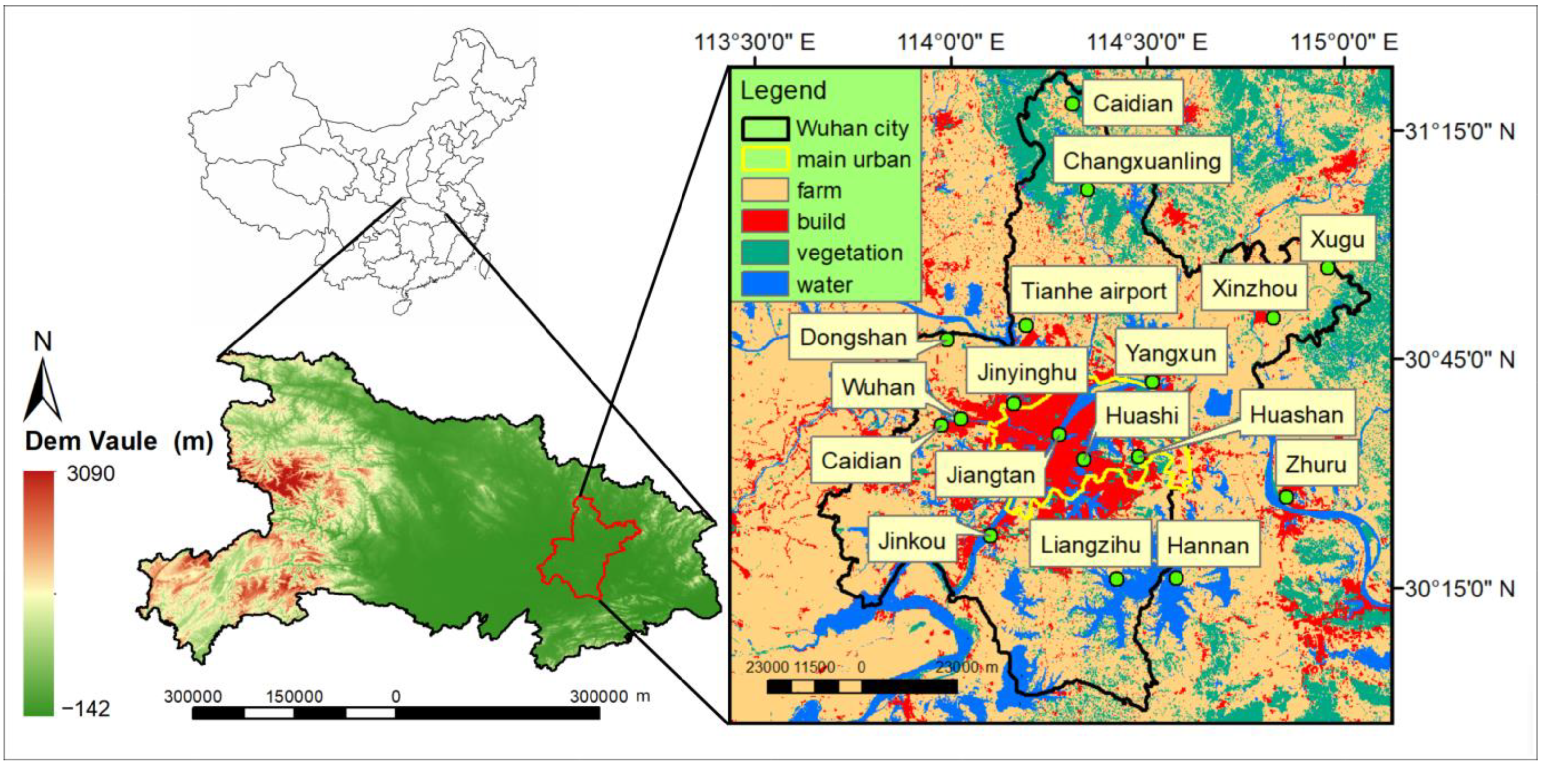
In this way, we obtained surface temperature and air temperature data for 17 sites on 13 cloudless days between 2013 and 2019. By combining this with the land-use distribution map, we matched the land use, surface temperature, and air temperature for each site, filtering out values with significant discrepancies. Ultimately, we obtained 233 data sets, with 84 sets from arable land, 77 from urban areas, 25 from vegetation, and 22 from water bodies. The land-use types and sample sizes for each site are detailed below (

Table 3. Meteorological Monitoring Points in Wuhan and Their Corresponding Land Surface Types.

Serial Number	Station	Number of Samples	Type
1	Wuhan	13	farmland
2	Caidian	13	built-up areas
3	Xinzhou	13	built-up areas
4	Jiangtan	10	water bodies
5	Huashan	12	vegetation
6	Huashi	12	built-up areas
7	Hannan	12	water bodies
8	Yangxun	13	farmland
9	Xugu	13	farmland
10	Tianhe airport	10	farmland
11	Caidian	13	vegetation
12	Changxuanling	13	farmland
13	Jinkou	9	farmland
14	Liangzihu	13	farmland
15	Dongshan	13	built-up areas
16	Jinyinhu	13	built-up areas
17	Zhuru	13	built-up areas

).

2.3.2. Prediction Methods for Land Surface Temperature and Air Temperature

To improve model accuracy, different LST–AT relationships were established for each land-use type using various modeling approaches.

• Regression Fitting

According to Agnieszka et al., the linearity of the LST–AT relationship depends on the built-up index [11]. Polynomial and exponential fitting methods were used, with models defined as follows:

$$AT=a_0+a_1\ast LST+a_2\ast {LST}^2+a_3\ast {LST}^3$$

(20)

$$AT=a_2\ast {LST}^{a_1}+a_0$$

(21)

where $a_0$, $a_1$, $a_2$, and $a_3$ are regression coefficients, AT is air temperature, and LST is land surface temperature. In traditional fitting, regression coefficients are determined by minimizing the sum of squared errors (SSE) between predicted and actual values using the least squares method.

2.

Random Forest (RF)

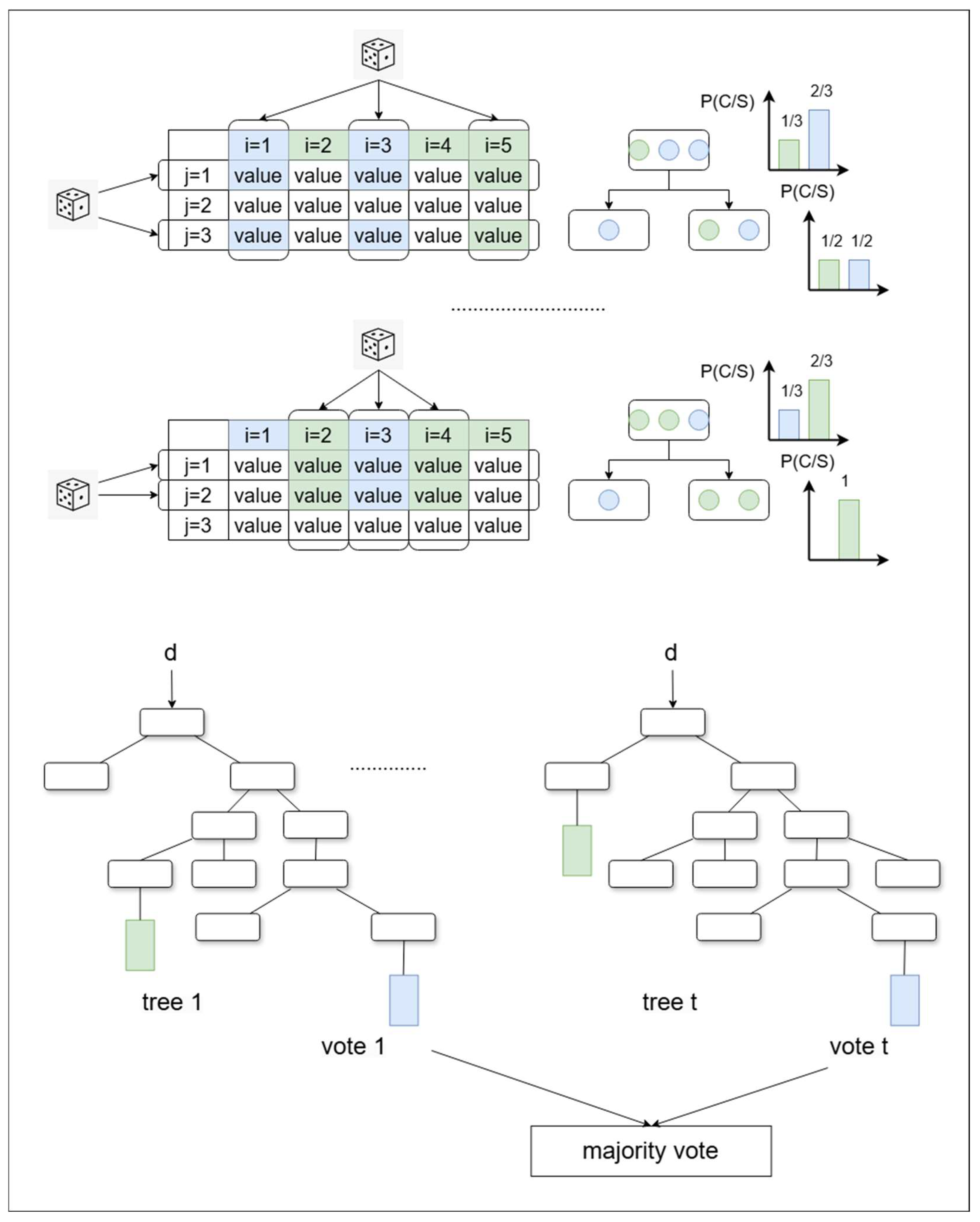
The Random Forest algorithm is an ensemble learning method primarily used for classification and regression tasks. It consists of multiple decision trees, improving model accuracy and robustness through ensemble learning. The steps of the Random Forest algorithm are as follows (Figure 5):

Initially, the Bootstrap Sampling method is employed to randomly extract multiple subsets (sample sets) from the original training dataset. Each subset is typically the same size as the original dataset, but sampling allows for duplicates. By providing different training data for each tree, the diversity of the model is increased, thereby enhancing the overall performance of the ensemble model.

Next, when training each decision tree, a random subset of features is selected from all available features. This random feature selection makes the constructed trees less correlated, allowing for more effective use of different features’ information and reducing the risk of overfitting.

Subsequently, decision trees are built using the selected feature subsets and sample sets. The tree construction process follows classic decision tree algorithms (such as CART) by selecting the best partition features to split the dataset into two subsets. This process stops when the subsets can no longer be split, a specific depth is reached, or other stopping criteria are met.

Finally, the Random Forest model is evaluated using metrics such as cross-validation and mean absolute error. Based on the assessment results, model parameters are tuned, including the number of trees, maximum depth, and minimum sample split size, to ensure that the model possesses good generalization capability [29].

In this study, the model type is first specified as regression. To ensure accuracy, the number of decision trees is set to 100. There are no restrictions on the maximum depth of the decision trees; by default, the trees will continue to grow until stopping conditions are satisfied (the sample count at each leaf node is less than the minimum leaf size), or all samples are completely split. The minimum leaf size is set to 3, requiring at least three samples at each node, which helps reduce model complexity and minimize overfitting risk. The feature function is left at its default setting, such that during each split, the model randomly selects the square root of the number of features for evaluation. The “Out-of-Bag” method is enabled to ascertain the importance of each feature’s contribution to the model.

3.

BP Neural Network

The backpropagation (BP) neural network is a feedforward neural network training algorithm that adjusts weights by backpropagating errors to minimize output errors. The steps of the BP neural network are outlined as follows (Figure 6):

First, the network parameters are initialized, determining the number of layers and the number of neurons in each layer. A BP neural network typically consists of an input layer, one or more hidden layers, and an output layer. Each connection’s weights and each neuron’s biases are randomly initialized to small values, ensuring sufficient learning capacity for the network.

Next, forward propagation occurs, where input data is fed into the network through the input layer. Once the input layer receives the data, the input signals are passed to the first hidden layer. Each neuron in the hidden layer calculates a weighted sum and computes its output using an activation function. After processing all hidden layers, the signal reaches the output layer, where the network output is calculated.

Following this, error evaluation occurs, calculating the error between the network output and the actual target values. Common metrics, such as Mean Squared Error (MSE), are used for this calculation. The calculated error is then backpropagated to compute the gradients of the weights concerning the error. Gradient descent algorithms, including Stochastic Gradient Descent (SGD), momentum, RMSProp, and Adam, are commonly used to adjust the weights.

The updated formula is as follows:

$$w_{new}=w_{old}-\eta ·\nabla E$$

(22)

where $w_{new}$ is the updated weight, $w_{old}$ is the original weight, $\eta$ is the learning rate, and $\nabla E$ is the error gradient.

After these steps are completed, forward propagation, error calculation, backpropagation, and weight updating are continuously repeated for each batch or the entire training dataset until the predefined number of training iterations (epochs), error thresholds are reached, or training is stopped based on validation set performance. Finally, independent data is used to validate the network’s generalization ability and prevent overfitting, assessing the model’s real-world application effectiveness [30].

In this study, the data is first normalized, scaling input and output data to the range of 0 to 1. The training set and test set are then divided in a 19:1 ratio. The hidden layer is set to have four neurons, creating a feedforward neural network. The hidden layer activation function uses the hyperbolic tangent function, while the output layer uses a linear function. The maximum number of iterations is set to 1000, with a learning rate of 0.01 and an error target of 1 × 10⁻⁶. Prediction performance metrics such as Root Mean Square Error (RMSE) and Absolute Error are calculated and displayed. Finally, the output data is denormalized to return to its original scale, with standard gradient descent used as the optimization algorithm. Due to the random nature of the path taken during training in the BP neural network, the results of each training session may differ. In this study, the error for this method is taken as the average value of 10 training sessions.

Given the relatively small sample size in this study, full-batch training was utilized. Importing the dataset once facilitates smoother convergence, while a more stable gradient update path may help find better local minima in certain situations, without significantly increasing computation time.

4.

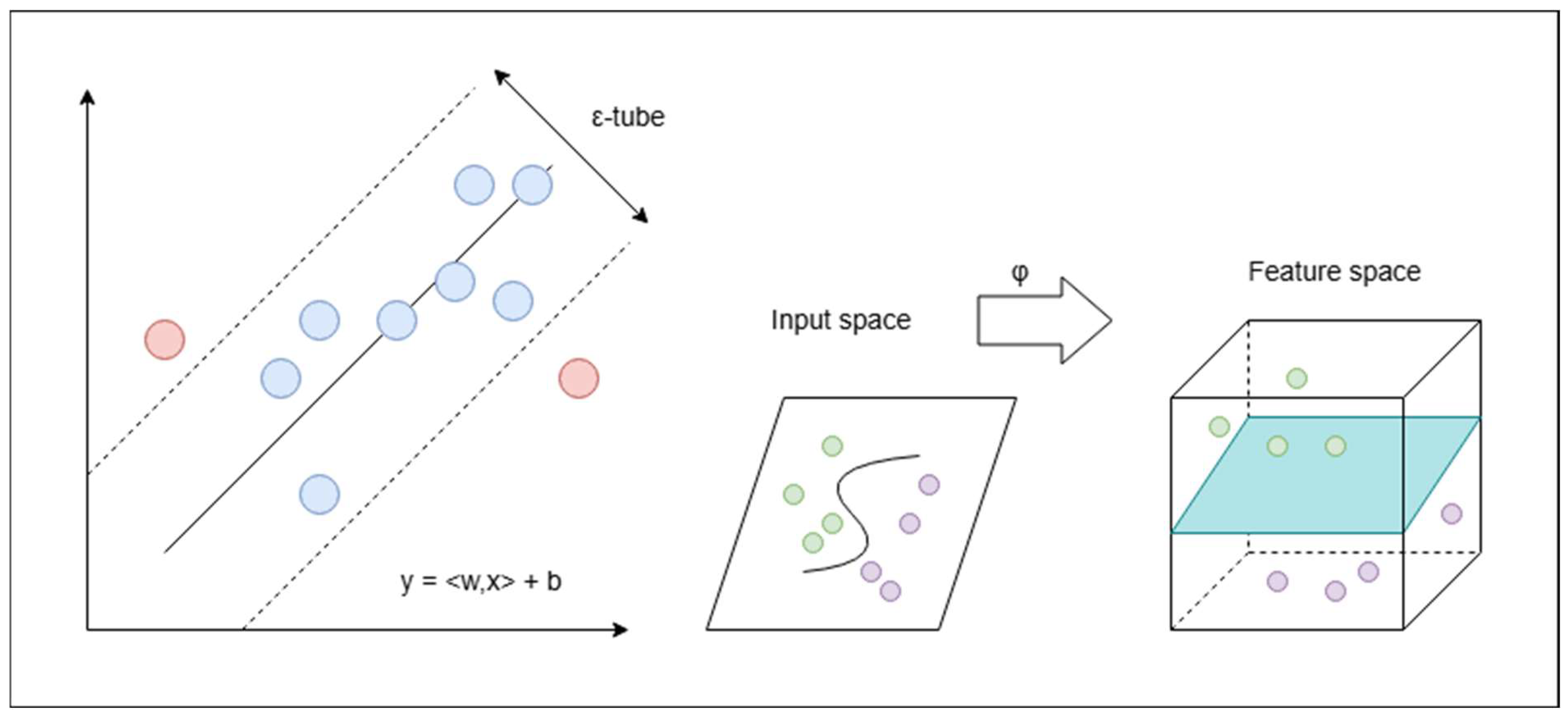
Support Vector Regression (SVR)

Support Vector Regression (SVR), based on Support Vector Machines (SVM), performs regression using a kernel function to enable nonlinear mapping of data [31]. Support Vector Regression (SVR) is a regression method based on Support Vector Machines (SVM). SVR attempts to find a function that can predict continuous target variables within a desired error range. The steps of SVR are as follows (Figure 7):

Data preprocessing is the initial step, preparing data for model training and testing, and selecting suitable features for modeling. The features are then scaled to ensure the convergence and stability of the model.

Next, an appropriate kernel function is chosen for the nonlinear mapping of the data. The choice of kernel function significantly impacts SVR’s performance. Common kernel functions include linear kernel, RBF kernel (Radial Basis Function), and polynomial kernel. Once the kernel function is determined, the model penalty parameter $C$ and insensitive loss function $\epsilon$ must be defined. The penalty parameter $C$ controls the model’s overfitting on training data and its generalization capability. A smaller $C$ increases tolerance for errors, while a larger $C$ aims for precise regression of training samples. The insensitive loss function $\epsilon$ defines a margin, allowing prediction errors less than $\epsilon$ not to incur penalties, reducing sensitivity to small errors.

The next step involves solving the optimization problem to identify the support vectors. SVR aims to minimize the following objective function by solving its Lagrange dual problem:

$${\displaystyle \frac{1}{2}}{\left|\left|w\right|\right|}^2+C\sum ({\xi }_i+{\xi }_i^{\ast })$$

(23)

where ${\xi }_i$ and ${\xi }_i^{\ast }$ are the slack variables for non-support vectors, and $w$ is the weight vector. This problem can be solved using suitable optimization algorithms, such as Sequential Minimal Optimization.

Finally, the model’s performance on the test set is evaluated using performance metrics such as Mean Squared Error (MSE) and R² to assess the effectiveness of the SVR model on the test set, thereby determining the model fit. Cross-validation can be employed to further validate the model’s performance and ensure its robustness.

In this study, the Radial Basis Function (RBF) is used as the kernel function. The penalty factor is set to 4.0, imposing stricter penalties on misclassifications, with the goal of reducing training errors. The kernel function parameter is set to 0.8, controlling the function’s width and thus the model’s complexity. The allowable error margin for the model is set at 0.01. After setting all parameters, the optimization is conducted using the Sequential Minimal Optimization algorithm. This algorithm simplifies the optimization problem by selecting two Lagrange multipliers, transforming the optimization issue into smaller sub-problems to be solved progressively, effectively utilizing memory and accelerating convergence. At each step, the algorithm selects two variables while fixing the others, converting the optimization problem into one regarding only these two variables.

3. Results

3.1. Land-Use Classification

To better describe the dynamics of land-use changes in Wuhan’s main urban area in terms of land-use characteristics and socioeconomic development, the analysis focused on areas with significant changes. The dynamics of land use in Wuhan’s main urban area from 2013 to 2019 are summarized in

Table 4. Land-Use Changes in Wuhan’s Main Urban Area (2013–2020).

Year/Type	2013 (km2)	2020 (km2)
farmland	332.37 (33.9%)	301.38 (30.8%)
vegetation	19.76 (2.0%)	20.86 (2.1%)
water bodies	189.1 (19.3%)	181.43 (18.6%)
built-up areas	427.67 (43.5%)	465.21 (47.5%)

. The distribution of land use from 2013 to 2019 is shown in Figure 8.

It was observed that cropland and built-up areas accounted for the majority of the land use within the study area, while water bodies constituted approximately 20%, and forested areas were the least represented. During this period, built-up areas continued to expand, with their proportion increasing from 43.5% to 47.5%. Meanwhile, water bodies saw a slight decrease from 19.3% to 18.6%, and vegetation proportions remained relatively stable. This indicates that urbanization in the study area has continued but at a slower pace compared to the period before 2013.

3.2. Land Surface Temperature

3.2.1. Summer Land Surface Temperature Distribution

Due to Wuhan’s monsoon climate, which is characterized by a significant temperature difference between winter and summer, the heat island and cool island effects are concentrated in the summer and winter, while they are not significant during the other periods. Therefore, the discussion will be divided into two parts. Summer is defined as the period from June to August, and winter is defined as December to February. However, due to limitations in cloud cover, only the cloud images from August and December can be used to represent summer and winter, respectively. Figure 9a shows the summer LST distribution in the main urban area of Wuhan in 2020. The data indicate a significant temperature range, with a maximum of 70 °C and a minimum of 24 °C, resulting in an average temperature of 44.8 °C. Although the maximum temperature within the study area is quite high, the areas experiencing extremely high temperatures are small in size. The vast majority of the region has temperatures ranging between 26 °C and 45 °C. Therefore, in the map, areas with temperatures above 45 °C are marked in red.

In terms of coverage, the strong heat island effect revealed by LST encompasses nearly the entire built-up area of the city. The heat island effect is particularly severe near Wuhan Station in the upper-central part of the city, likely due to the presence of industrial bases and transportation hubs in these areas. The release of waste heat alone can cause a substantial temperature rise. Comparing these urban heat island zones with the rural average temperature (38 °C) reveals that the heat island intensity derived from LST can reach 32 °C in the most affected areas.

In addition to built-up areas and cropland, vegetation also merits attention. Although Wuhan has scattered vegetation patches, their temperatures are comparable to cropland and have limited impact on the surrounding thermal environment. This indicates that dispersed vegetation provides minimal relief from the heat island effect [32].

Water bodies and vegetation exhibit similar cooling trends. Smaller, fragmented lakes near the city center have an average LST of 35 °C, with weak surrounding cooling effects, while the Yangtze River, which traverses the city, maintains an average LST of 30 °C. Temperatures in areas near the river are significantly lower than those in the surrounding regions. This difference likely arises from the higher thermal capacity of larger lakes and rivers, which allows them to absorb heat more effectively [33].

Overall, LST observations indicate the following heat island intensity hierarchy: built-up areas > cropland > vegetation > water bodies. While the heat island effect is pronounced in built-up areas, vegetation’s cooling effect is minor, whereas water bodies display a notable cooling effect.

3.2.2. Winter Land Surface Temperature Analysis

Figure 9b illustrates the winter LST distribution in Wuhan’s main urban area in 2020. Unlike summer, winter exhibits a different pattern of heat and cold island distribution. The temperature range is smaller in winter, with a maximum of 24.8 °C, a minimum of −0.8 °C, and an average of 10.9 °C.

The average LST of built-up areas is 0.5 °C lower than that of cropland, suggesting the presence of a cold island rather than a heat island in the city center. Furthermore, the smaller temperature span and uniform distribution indicate a milder heat island effect in winter compared to summer. The distribution pattern of heat islands also changes, with strong heat islands appearing not only in industrial and transportation hub areas but also in Tianxingzhou, an island at a fork of the Yangtze River.

Industrial heat islands are likely caused by waste heat from factories, while the heat island effect on Tianxingzhou may stem from the river’s flow facilitating water circulation. Flowing water can carry heat and mitigate cooling, while increased fog formation creates an insulating layer that slows heat loss, keeping the island relatively warm.

Vegetation displays a cold island effect in winter, likely due to reduced biological activity. Transpiration and respiration rates drop significantly, especially for deciduous plants.

Water bodies exhibit notable seasonal differences. In both summer and winter, rivers maintain an approximately 5 °C higher average temperature than lakes. This disparity may be attributed to the higher flow rates of rivers, which enable continuous heat exchange via convection and diffusion. Additionally, rivers receive inflows from regions with varying temperatures and have larger surface areas to absorb solar radiation, preventing rapid cooling like static water bodies [34].

Overall, winter LST varies greatly among land-use types. A single land-use type may act as a heat island or a cold island depending on specific site conditions.

3.3. Validation of Air Temperature Prediction Model Accuracy

Using the methods described above, five models were developed for each of the four land-use types to predict the relationship between LST and AT.

Table 5. Error Analysis of the Five Models.

Method Category	Land-Use Type	MSE	R2
Polynomial Fitting	built-up areas	2.739	0.904
	farmland	2.77	0.902
	vegetation	2.283	0.915
	water bodies	2.189	0.905
Exponential Fitting	built-up areas	3.081	0.877
	farmland	2.961	0.887
	vegetation	2.386	0.937
	water bodies	3.111	0.892
Random Forest	built-up areas	1.885	0.942
	farmland	1.856	0.953
	vegetation	2.463	0.924
	water bodies	4.127	0.784
BP Neural Network	built-up areas	1.992	0.923
	farmland	2.156	0.907
	vegetation	2.375	0.907
	water bodies	2.521	0.895
SVR	built-up areas	2.441	0.92
	farmland	2.873	0.889
	vegetation	2.229	0.905
	water bodies	2.917	0.885

summarizes the prediction errors for each model.

$$SSE={{\sum }_{i=1}^n(y_i-{\widehat{y}}_i)}^2,MSE={\displaystyle \frac{SSE}{n}},RMSE=\sqrt{MSE},R^2=1-{\displaystyle \frac{SSE}{{\sum _{i=1}^n(y_i-\overline{y})}^2}},$$

where ${\widehat{y}}_i$ represents the predicted value, $y_i$ represents the actual value, $n$ is the sample size, and $\overline{y}$ is the mean of the actual values.

Based on the error analysis, the model with the highest coefficient of determination (R²) for each land-use type was selected as the final model. Polynomial fitting was chosen for water bodies (R² = 0.905), while the random forest algorithm was used for the remaining types: built-up areas (R² = 0.942), cropland (R² = 0.953), and vegetation (R² = 0.924). Using the selected models, calculations were performed separately for each land-use type. Furthermore, even if a model performs well in error analysis, it may perform poorly when predicting new data. Therefore, actual calculations are needed to determine whether the model has sufficient generalization capability. Therefore, in Section 3.4.1, we re-evaluate the model by actually plotting the air temperature cloud map.

3.4. Air Temperature Mapping

3.4.1. Generation of Air Temperature Maps

After establishing preliminary models, the models were applied to retrieve temperature data from remote sensing images and generate air temperature maps. However, discrepancies were observed between modeled and measured data for built-up areas in summer and water bodies in winter. To address this, a secondary model (BP neural network) was used as an alternative, yielding improved results (Figure 10).

By comparing LST and AT maps, it is evident that both indicate higher temperatures in industrial zones within the city center compared to surrounding areas. Regarding the effects of land-use types on thermal environments, both LST and AT reveal consistent trends, differing only in the intensity of the urban heat island (UHI).

In summer, the maximum AT in Wuhan’s main urban area reached 44.8 °C, the minimum was 28.8 °C, and the average was 33.9 °C. The UHI intensity derived from LST reached a peak of 32 °C, while the highest AT-derived UHI intensity was only 11 °C. Furthermore, areas of high UHI intensity were limited to industrial zones. These findings align with Zander et al., who concluded that LST-based assessments significantly overestimate UHI intensity compared to AT-based assessments [35].

In winter, the maximum AT in Wuhan’s main urban area was 20.6 °C, the minimum was 0.7 °C, and the average was 7.8 °C. The distribution of thermal environments reflected by LST and AT was similar, and the discrepancies between the two were much smaller than in summer. The differences in UHI intensity between LST- and AT-based assessments were negligible, suggesting that LST can be directly used for UHI studies in winter without significant loss of accuracy.

The discrepancies in map accuracy arose from the nature of the random forest algorithm. This method predicts outcomes based on localized rules from training data. When input data fall outside the training range, random forest models struggle to provide accurate predictions. In this study, measured data ranged from 5 °C to 45 °C. However, in summer, the LST of built-up areas and cropland exceeded this range, and in winter, the temperature of lakes fell below it. Out-of-range data were flagged as invalid in the air temperature maps. This issue reflects the challenge of using a training dataset of only a few hundred samples to model millions of pixels. Additionally, the random forest algorithm is limited to adjusting tree count and depth, making fine-tuning more challenging [36].

In contrast, the BP neural network effectively addresses these issues. First, LST and AT are continuous physical variables, and BP neural networks excel at fitting continuous functions. Unlike the decision tree-based segmentation of random forests, BP neural networks better capture and model the smooth relationships between inputs and outputs. This enables reasonable predictions even for out-of-range input data, avoiding the extreme results produced by random forests. Second, BP neural networks offer a wide range of tunable parameters, including the number of hidden layers, neurons per layer, activation functions, and learning rates. This flexibility allows the model to more accurately reflect real-world conditions [37].

3.4.2. Comparison Between Predicted Values and Actual Values

To evaluate the accuracy of the air temperature maps, predictions were compared with actual measurements on six days in 2020. Using the trained models and LST maps, spatially continuous air temperature maps were generated.

$$SSE={{\sum }_{i=1}^n(y_i-{\widehat{y}}_i)}^2,MSE={\displaystyle \frac{SSE}{n}},RMSE=\sqrt{MSE},\mathrm{M}\mathrm{A}\mathrm{E}={\displaystyle \frac{1}{n}}{\sum }_{i=1}^n\mid y_i-{\widehat{y}}_i\mid ,$$

$$\mathrm{COR}={\displaystyle \frac{{\sum }_{i=1}^n\left(y_i-\overline{y}\right)\left(\widehat{y_i}-\overline{\widehat{y}}\right)}{\sqrt{{\sum }_{i=1}^n{\left(y_i-\overline{y}\right)}^2\cdot {\sum }_{i=1}^n{\left(\widehat{y_i}-\overline{\widehat{y}}\right)}^2}}},R^2=1-{\displaystyle \frac{SSE}{{\sum _{i=1}^n(y_i-\overline{y})}^2}},$$

where ${\widehat{y}}_i$ represents the predicted value, $y_i$ represents the actual value, $n$ is the sample size, and $\overline{\widehat{y}}$ and $\overline{y}$ are the mean values of the predicted and actual values (

Table 6. Error Analysis of the Final Models.

Method Category	Number of Samples	R2	SSE	MSE	MAE	RMSE	COR
BP Neural Network-farmland	42	0.8872	405.7767	9.6614	2.6385	3.1083	0.95
BP Neural Network-built-up areas	30	0.86226	348.8008	11.6267	3.021	3.4098	0.94
BP Neural Network-vegetation	12	0.85466	101.9875	8.499	1.9234	2.9153	0.94
Polynomial Fitting-water bodies	12	0.87293	150.9664	12.5805	2.8031	3.5469	0.95
Total	96	0.8762	1007.5314	10.4951	2.6892	3.2396	0.94

).

Error analysis revealed that the R² values for all land-use types exceeded 0.85, indicating that the models effectively captured the relationship between LST and AT. Comparing water bodies and cropland with similar sample sizes, it was observed that the BP neural network achieved lower R² and mean absolute error (MAE) values than polynomial fitting. This suggests that the BP neural network better fits the overall trend of the data and provides a more comprehensive explanation of the LST–AT relationship, though it was slightly less accurate in terms of prediction precision.

Figure 11 illustrates that model errors were lower during summer and winter but higher during transitional seasons (with measured values ranging between 15 °C and 30 °C). This is likely due to the region’s frequent and intense climate changes during transitional seasons, which are challenging for models to capture accurately.

4. Discussion

• The influence of different land-use types on the thermal environment revealed by surface temperature and air temperature is consistent, with the phenomenon of heat island intensity being built-up areas > arable land > vegetation > water bodies [38]. However, the surface temperature in built-up areas is much higher than the air temperature, and cool islands in vegetation are not evident, while water bodies show pronounced surface and air-cool islands. During summer, the surface heat island indicates that there is a widespread strong heat island in Wuhan’s main urban area, with both heat islands and cool islands being very distinct, and there are significant temperature differences between various urban regions. Yet, the summer air heat island shows that most areas in the main urban area do not have heat islands, with strong heat islands confined to a small area, indicating that there is a significant disparity between evaluations based on surface temperature and air temperature in summer. Relying solely on one type for assessment may lead to erroneous policies; both measurement methods must be taken into account.
• The distribution of heat/cool islands in winter differs significantly from that in summer. Whether based on surface temperature or air temperature, the average temperature in built-up areas is 0.5 °C lower than that in arable land, indicating the presence of cool islands in the city center rather than heat islands. However, the occurrence of cool islands in winter is not conducive to human thermal comfort, suggesting that the thermal environment in the study area is not ideal. Vegetation displays both heat islands and cool islands in winter, which may not be due to differences in the thermal regulation capacity of the plants themselves but rather due to the duration of sunlight exposure [39]. Most plants experience restricted life activities in winter, with significantly reduced transpiration, particularly for deciduous plants [40]. Differences among various water bodies in winter are considerable, with average temperature differences between rivers and lakes exceeding 5 °C for both surface and air temperatures. This phenomenon may arise because rivers, compared to lakes, have higher flow rates, allowing heat to be continually exchanged through diffusion and convection due to the flow [41]. Overall, the thermal environment distribution reflected by surface temperature and air temperature in winter is very similar, without the significant differences seen in summer. The temperature differences between the two measurements in various regions are quite close, and the variation in heat island intensity assessed using surface temperature and air temperature is minimal. Both heat islands and cool islands exhibit consistent geographical distributions. This indicates that directly using surface temperature to study winter heat islands may not have a significant impact.
• Error analysis shows that polynomial fitting achieves an R² of around 0.9, while the R² of machine learning models correlates positively with sample size. When sample sizes are small, R² may fall below 0.8, but with sufficient data, it can exceed 0.95. Therefore, polynomial fitting is preferable for small sample predictions, while machine learning methods are better suited for large datasets.
• For the specific task of modeling the LST–AT relationship, the availability of AT data is often limited due to reliance on meteorological stations or manual measurements. Data continuity is further constrained by satellite revisit periods and cloud cover, while air temperature above water bodies is particularly challenging to obtain. These limitations result in a restricted sample size and range. If the sample range cannot cover the required prediction range, BP neural networks are recommended due to their ability to generalize beyond the training data range [42]. If sufficient samples are available to cover the prediction range, random forests perform better based on error analysis.
• Further discussion can be made regarding the predicted results. As shown in Figure 10, if we categorize the predicted values and actual values into high temperatures (above 25 °C) and low temperatures (below 25 °C), it becomes apparent that the model effectively reflects the trends under low-temperature conditions. However, it exhibits considerable fluctuations under high-temperature conditions, with the maximum temperature difference reaching 8 °C for the set that deviates the most. This situation may be attributed to the differing natural conditions between winter and summer.
  In summer, solar radiation is intense, and the longer daylight hours result in a more vigorous heat exchange between the surface and the air, leading to a rapid increase in surface temperature. Simultaneously, increased summer precipitation may intensify air convection, causing temperature fluctuations [43].
  Conversely, winter exhibits relatively high humidity, with abundant moisture in the air, possibly influencing the relationship between air temperature and surface temperature through the interaction of temperature and humidity, resulting in more consistent low-temperature characteristics.
  Therefore, future improvements to the model need to consider the complexities during high-temperature periods, possibly by increasing the sample size or adding additional variables for prediction.

5. Conclusions

This study aimed to establish a method for obtaining spatially continuous air temperature data using only LST by modeling the relationship between LST and AT across different land-use types. The findings are as follows:

• LST maps revealed the following UHI intensity hierarchy in summer: built-up areas > cropland > vegetation > water bodies. Built-up areas exhibited a strong heat island effect, vegetation provided minimal cooling, and water bodies demonstrated a significant cooling effect. In winter, temperatures varied widely across land-use types, and a single type could manifest as either a heat or cold island depending on its specific characteristics.
• Polynomial regression performed best for water bodies (R² = 0.905), while random forests achieved the highest R² for built-up areas (R² = 0.942), cropland (R² = 0.953), and vegetation (R² = 0.924).
• Air temperature maps generated using the established models and LST data showed that relying solely on LST significantly overestimates UHI intensity in summer. In winter, differences between LST- and AT-based UHI intensities were minimal, suggesting that LST can be directly used to evaluate UHI effects under resource constraints.
• Comparisons between predicted and observed air temperatures revealed high accuracy in summer and winter but lower accuracy during transitional seasons. This discrepancy likely results from the region’s highly variable climate during these periods, requiring larger datasets to improve model performance.