Abstract
This study presents a comprehensive analysis of the impact of Storm Laura, which was observed over Europe and the Baltic Sea on 12 March 2020, on the thermosphere–ionosphere system. The investigation of ionospheric disturbances caused by the meteorological storm was carried out using a combined modeling approach, incorporating the regional AtmoSym and the global GSM TIP models. This allowed for the consideration of acoustic and internal gravity waves (AWs and IGWs) generated by tropospheric convective sources and the investigation of wave-induced effects in both the neutral atmosphere and ionosphere. The simulation results show that, three hours after the activation of the additional heat source, an area of increased temperature exceeding 100 K above the background level formed over the meteorological storm region. This temperature change had a significant impact on the meridional component of the thermospheric wind and total electron content (TEC) variations. For example, meridional wind changes reached 80 m/s compared a the meteorologically quiet day, while TEC variations reached 1 TECu. Good agreement was obtained with experimental TEC maps from CODE (Center for Orbit Determination in Europe), MOSGIM (Moscow Global Ionospheric Map), and WD IZMIRAN (West Department of Institute of Terrestrial Magnetism, Ionosphere and Radio Wave Propagation Russian Academy of Sciences), which revealed a negative TEC value effect over the meteorological storm region.
1. Introduction
The study of the influence of processes occurring in the neutral atmosphere on the state of the ionosphere is an important task. The ionosphere is affected by numerous heliophysical processes both from above and below [1]. The ionospheric response to disturbances propagating from below remains one of the key topics in ionospheric research. Similarly to the ionospheric response to geomagnetic disturbances, variations in the thermosphere–ionosphere system during intense meteorological storms in the troposphere can reach up to 20% [2,3]. Meteorological events, such as tropical cyclones, contribute to the transfer of heat, energy, and mass, thereby playing a crucial role in maintaining thermal equilibrium in the atmosphere and at the ocean surface [4,5,6]. Meteorological phenomena, particularly strong tropospheric convection, are generally believed to generate a broad spectrum of acoustic waves (AWs) and internal gravity waves (IGWs). These include IGWs with scales ranging from tens to hundreds of kilometers and periods from 5 min to several hours. These waves propagate upward and reach thermospheric altitudes, increasing amplitudes by two orders of magnitude due to the decrease in the medium density. This amplification can lead to the development of nonlinear processes before dissipation occurs, influencing the parameters of the thermosphere–ionosphere system [7,8,9,10,11,12,13]. Recent studies incorporating experimental data from satellite [14] and vertical sounding [15], global navigation satellite system (GNSS) observations [11,16,17], as well as numerical modeling results [18,19], indicate a wave coupling between different atmospheric layers. Atmospheric gravity waves, particularly AWs and IGWs, propagating from meteorological storm regions, have a significant impact on the ionosphere and can lead to plasma instabilities [11,20,21]. The most common and frequently observed ionospheric response to such waves is the formation of traveling ionospheric disturbances (TIDs).
Meteorological convective events generate atmospheric waves with a wide range of wavelengths. To determine the characteristic features of the atmospheric and ionospheric response to such events, a detailed analysis of a sufficient number of cases is required. In this study, a meteorological storm over the Baltic Sea in March 2020 was selected for analysis. The aim of this research was to perform a numerical study of the propagation of AWs and IGWs from a tropospheric source with the subsequent detection of the same waves in experimental data to confirm changes in TEC due to their heating of the thermosphere.
2. Modeling Methodology and Processing of Experimental Data
Experimental methods for studying the impact of meteorological storms on the thermosphere and ionosphere, including satellite observations, do not always allow for the isolation of the meteorological effects on thermospheric and ionospheric parameters due to the lack of sufficient high-resolution spatial and temporal data. To gain a more detailed understanding of the thermosphere–ionosphere system, it is necessary to further develop mathematical modeling methods. A significant number of global upper atmosphere models exist; however, most of them are unable to reproduce the effects of processes occurring in the lower atmosphere [22]. In recent years, several high-resolution regional models have been actively developed, enabling the consideration of lower atmospheric processes in the state of the thermosphere–ionosphere system. In this study, ionospheric disturbances caused by meteorological events in the troposphere were studied using both experimental data and regional AtmoSym and global GSM TIP models.
2.1. Modeling of TEC Variations in the GSM TIP During a Meteorological Storm
During a meteorological storm, AWs and IGWs propagate from the disturbance region. Reaching the heights of the lower thermosphere, they effectively dissipate, causing heating of the neutral gas. The increase in the neutral component temperature Tn leads to significant changes in the composition and dynamics of the thermosphere, which also affects the variations in ionospheric parameters—in particular, the TEC.
To numerically determine the temporal variations in TEC, we employed a comprehensive approach [23] that accounts for the propagation of AWs and IGWs generated by a tropospheric meteorological source. Figure 1 presents a schematic representation of the main stages of this approach. In Figure 1, is experimentally obtained pressure variations, which are used in the calculations as the lower boundary condition.
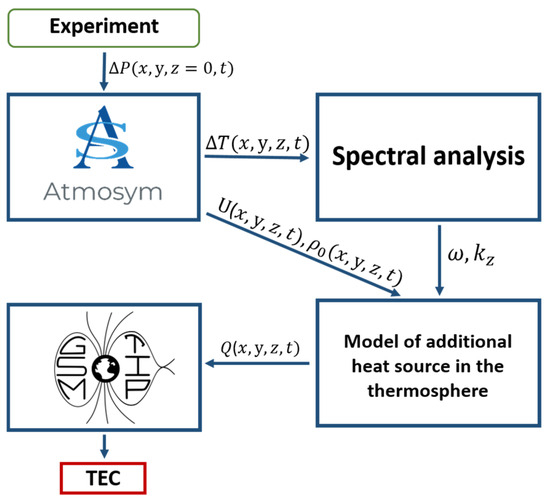
Figure 1.
Schematic representation of the comprehensive approach for determining model TEC variations during a meteorological storm.
At the first stage, wave propagation from the meteorological source is modeled using the regional numerical model AtmoSym [24]. AtmoSym is a high-resolution neutral atmosphere model that describes the propagation of AWs and IGWs while accounting for nonlinear and dissipative processes. The numerical method used enables accurate calculations of infrasonic and internal gravity wave behavior over several tens of hours. AtmoSym is a non-hydrostatic model and operates at altitudes z from 0 to 500 km.
Previously, in [25], a uniqueness theorem was proven for a problem where pressure variations are specified as the lower boundary condition. Therefore, following [25], the AtmoSym model can incorporate experimental microbarograph data on surface pressure variations (at altitude z = 0) during meteorological storms with wind gusts exceeding 25 m/s.
The output of the AtmoSym model consists of time-dependent three-dimensional fields of scalar and vector hydrodynamic functions, which allow for the estimation of disturbance amplitudes in the upper atmosphere caused by waves from an atmospheric front. At the second stage, the temperature variations obtained from the AtmoSym calculations are used to determine their frequencies ω and vertical wavenumbers via windowed Fourier analysis. The spectral characteristics such as ω and , along with the horizontal velocity and background density of the medium parameters, calculated by AtmoSym at different locations and time moments, enable the determination of the wave-induced heat flux density in the atmosphere [26]:
where is the amplitude of horizontal velocity oscillations, and β .
In the third stage, is converted into the heating rate . The value of is then used as an input parameter for the Global Self-Consistent Model of the Thermosphere, Ionosphere, and Protonosphere (GSM TIP) [27,28], where it is included as an additional term in the thermal balance equation for neutral components.
The GSM TIP model is based on the numerical integration of a system of quasi-hydrodynamic equations, including continuity, momentum, and thermal balance equations for neutral and charged particles in the cold near-Earth plasma, along with the equation for the electric potential. It operates within an altitude range from 80 km to a geocentric distance (~15 Earth’s radius), taking into account the mismatch of geographical and geomagnetic axes. GSM TIP provides global distributions of temperature, the components of the mass-averaged velocity vector, and the concentrations of neutral components in the Earth’s upper atmosphere (O2, N2, O, NO, N(2D), N(4S)). It also calculates the temperature, velocities, and densities of atomic (O⁺, H⁺) and molecular ions (N₂⁺, O₂⁺, NO⁺), as well as electrons. Additionally, it provides the two-dimensional distribution of the electric potential arising from ionospheric and magnetospheric sources. At the fourth and final stage, the GSM TIP model produces global TEC distribution maps, generated at predefined time intervals.
2.2. TEC Measured Using GNSS Data
Methods based on the reception and processing of signals from GNSS are widely used to study spatial and temporal variations in ionospheric parameters. In particular, these observations provide spatial and temporal distributions of TEC. Global and regional TEC maps are highly valuable for studying the ionospheric response to various geophysical disturbances. Currently, several centers generate global and regional TEC maps [29,30]. In this study, to analyze the ionospheric state during the meteorological storm, we utilized TEC maps from the CODE (Center for Orbit Determination in Europe) [31], MOSGIM (Moscow Global Ionospheric Map) [32], and the WD IZMIRAN (West Department of Institute of Terrestrial Magnetism, Ionosphere and Radio Wave Propagation Russian Academy of Sciences) [33,34]. Table 1 presents the key characteristics of the TEC maps produced by these centers.

Table 1.
Key characteristics of the TEC maps used in this study.
To identify the ionospheric effects caused by tropospheric processes, we analyzed the difference between vertical TEC values obtained from observations on 12 March 2020 (a meteorologically disturbed day) and 10 March 2020 (a meteorologically quiet day).
3. Results and Discussion
3.1. Description of Storm Laura and the Helio-Geophysical Conditions During Its Passage
Storm Laura hit Denmark and southern Sweden on 12 March 2020. It was named Laura by the Danish Meteorological Institute, and is known as Hanna by the Free University of Berlin. It originated in the North Atlantic and caused meteorological disturbances, with wind gusts exceeding 30 m/s over the North and Baltic Seas, and with maximum gusts reaching 38 m/s. The storm moved rapidly, reaching the southern Baltic within a several hours. Figure 2 shows the trajectory of this storm over Europe.
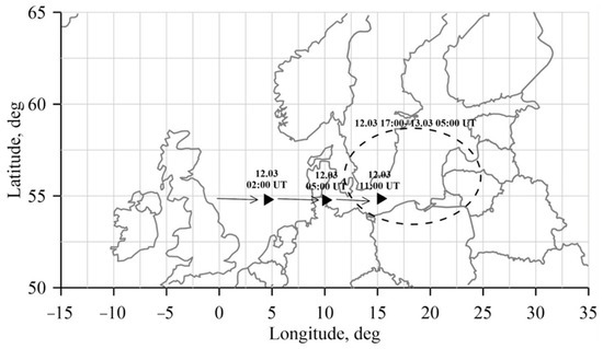
Figure 2.
Schematic representation of Storm Laura’s movement on 12 March 2020. The dashed line indicates the characteristic region of meteorological disturbances over the Baltic Sea during Storm Laura.
When studying the impact of intense meteorological events on the thermosphere–ionosphere system, it is essential to rule out other geophysical factors that could significantly influence the state of the ionosphere, particularly solar and geomagnetic activity. Figure 3 presents solar and geomagnetic activity data for 5–20 March 2020. As shown in Figure 3, the heliogeophysical conditions remained quiet throughout the study period. The Kp index did not exceed 3, the Dst index remained above −20 nT and showed no significant daily variations, and the F10.7 solar flux index remained stable in the range of 68–72 s.f.u. During the period we considered, there was a slight increase in geomagnetic activity, as can be determined from the changes in the geomagnetic indices Kp and Dst. Additional information on the dynamics of the disturbance at high latitudes and its strength can be obtained from variations in the temperature of solar wind protons and the Ey component of the interplanetary electric field [34,35]. It can be seen that the evolving geomagnetic perturbation is small and its influence on the midlatitude ionosphere is insignificant, so one can conclude that the perturbations in the upper atmosphere and ionosphere observed in the region under consideration are mainly a consequence of the tropospheric processes.
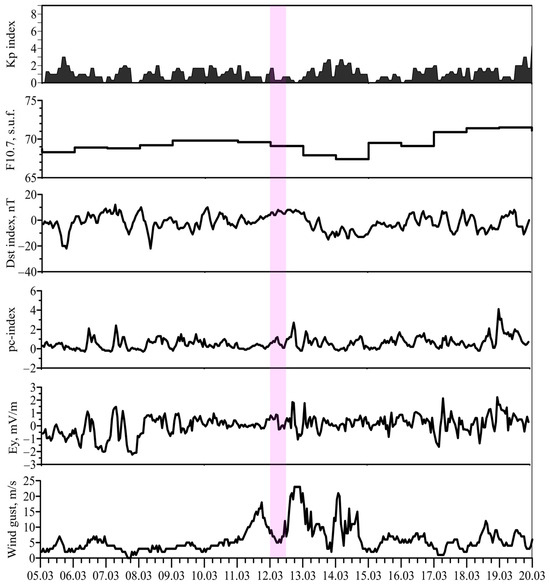
Figure 3.
Geomagnetic activity indices (Kp, Dst), F10.7 solar flux, and wind gust speed in Kaliningrad (54°53′ N, 20°35′ E) from 5 March to 20 March 2020. The area highlighted in pink indicates the time period under study.
The lower panel of Figure 3 presents wind speed observations at Khrabrovo Airport, Kaliningrad (54°53′ N, 20°35′ E). It is noted that, on the afternoon of 11 March, wind gusts increased to 15 m/s, reaching their peak (over 20 m/s) in Kaliningrad on the afternoon of 12 March. Thus, one can assume that the disturbances in the upper atmosphere and ionosphere observed during this period were a direct consequence of tropospheric processes.
3.2. Results of GSM TIP Modeling
In this modeling study, three numerical experiments were performed using the GSM TIP model: a simulation for 12 March 2020, without including a heat source from atmospheric wave propagation (M1); a simulation for 12 March 2020, with a heat source associated with atmospheric wave propagation (M2); and a simulation for 10 March 2020, without a heat source from atmospheric wave propagation (M3). All numerical calculations were performed with a time step of 1 min.
To isolate the effects of adding a thermal source associated with propagating atmospheric waves, the differences between the results of M2–M1 and M2–M3 were analyzed at the background geomagnetic conditions. Since the geomagnetic conditions remained non-disturbed between 10 March and 12 March, the results of M2–M1 and M2–M3 were found to be very similar. Therefore, further analysis focuses only on M2–M3, allowing us to effectively isolate and assess the contribution of atmospheric waves initiated by the meteorological source.
Figure 4 presents the latitude–longitude distribution of temperature disturbances at 02:00, 04:00, and 06:00 UT on 12 March 2020, at an altitude of 294 km. Note that one of the reasons for choosing the altitude of 294 km is that it is a node of the calculation grid of the GSM TIP model. Moreover, no significant difference was observed compared to the nearest nodes. As seen in Figure 4, at 02:00 UT, a temperature increase (ΔT) forms over the meteorological storm region, reaching a maximum of ΔT = 40 K. By 04:00 UT, the area of elevated temperature is localized between 45 and 60° N and 10–25° E, with a peak disturbance exceeding ΔT = 100 K. Later, at 06:00 UT, the amplitude of disturbances decreases, and the perturbation region shifts westward.
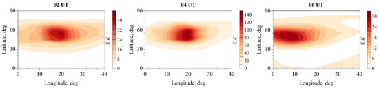
Figure 4.
Latitude–longitude distribution of temperature disturbances at an altitude of 294 km, caused by wave propagation (M2–M3 difference) at 02:00, 04:00, and 06:00 UT.
The neutral wind, particularly its meridional component, can also be a source of ionospheric changes, including TEC variations. At F-region altitudes, the meridional wind plays a crucial role in the overall dynamics of the thermosphere [36]. Figure 5a presents the latitude–time variation in the meridional wind , calculated as follows:
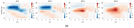
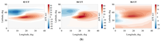
Figure 5.
(a) Latitude–time distribution of meridional wind variations at an altitude of 294 km at different longitudes; (b) latitude–longitude distribution of meridional wind variations at 294 km, induced by the additional heat source (M2–M3 difference) at 02:00, 04:00, and 06:00 UT.
At 20° E longitude, an increase in the meridional wind is observed starting from 02:00 UT, reaching values of 80 m/s. At 30° E longitude, the region of enhanced meridional wind perturbations persists; however, the amplitudes are significantly lower, not exceeding 45 m/s. At 10° E longitude, the meridional wind perturbation is negative at latitudes above 55° N until 05:00 UT, after which it changes sign. At latitudes below 55° N, the meridional wind perturbations remain positive.
The wind variations exhibit a rather complex pattern. When analyzing the latitude–longitude structure of the wind at different time instants (see Figure 5b), a structured pattern forms over the perturbation region in the lower atmosphere at 02:00 UT and 04:00 UT. A detailed mechanism for the formation of this structure is described in [23]. By 06:00 UT, the wind structure appears to change, and only a positive effect is observed.
3.3. TEC Maps and Spectra
Analysis of latitude–time model TEC variations at different longitudes (see Figure 6) reveals that, one hour after the activation of the heat source, a negative effect formed at latitudes 55–75° N across all considered longitudes. The maximum negative effect is observed at 20° E, localized north of the perturbation region, reaching 0.8 TECu. The maximum positive effect appears south of the perturbation region four hours after the heat source activation. At 10° E and 30° E, the regions with negative effects are smaller, and the values do not exceed 0.3 TECu. The calculated TEC values varied in interval 5–7 TECu during a reference time.
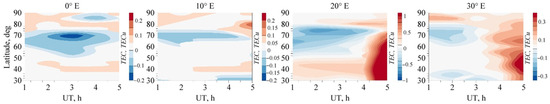
Figure 6.
Latitude–time distribution of model TEC disturbances at different longitudes.
Figure 7 presents the regional TEC maps obtained from experimental data (CODE, MOSGIM, WD IZMIRAN) and modeling results (GSM TIP model). All maps show a similar negative TEC effect in the European sector, reaching 2–3 TECu in the experimental data and up to 1 TECu in the modeling results. Such a difference between the experimental and calculated values may be due to the insufficient power of the model tropospheric source. This may happen for two reasons. On the one hand, not all tropospheric parameters were available to us. On the other hand, the experimental data on TEC variations differ significantly from each other. The above did not allow us to adjust the source power. However, the general trends in the manifestation of ionospheric disturbances in our calculations are reflected correctly. The localization of the negative effect differs slightly, likely due to differences in the map generation techniques.
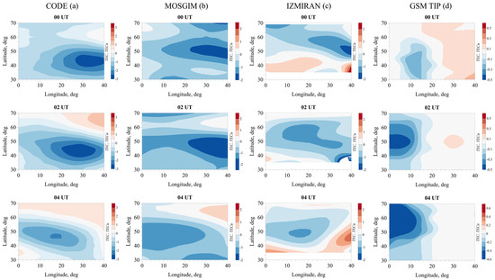
Figure 7.
TEC differences between the meteorologically disturbed day (12 March 2020) and the meteorologically quiet day (10 March 2020), based on the following: (a) GIM TEC CODE; (b) GIM TEC MOSGIM; (c) regional European TEC maps from IZMIRAN; (d) GSM TIP model. Data are shown for 02:00 UT, 04:00 UT, and 06:00 UT.
A comparison of the modeled results and experimental data shows that the negative effect is present in both, but the amplitudes and localization of the disturbances differ. The modeled disturbance amplitudes are 1–2 TECu lower than those observed in the experimental data. It is important to note that the localization of negative effects depends on the position, intensity, and duration of the heat source.
Studies [15,37] based on the analysis of data from individual GNSS satellite signal reception stations and remote sensing stations have suggested that, during strong meteorological disturbances, TEC variations are primarily driven by thermospheric wave processes of tropospheric origin. The mechanism explaining this effect is typically associated with the heating of neutral gas due to wave dissipation in the thermosphere, leading to subsequent changes in neutral gas composition and dynamics. The perturbation region observed in the TEC maps extends beyond the spatial scale of the meteorological storm in the troposphere, which is attributed to the propagation characteristics of IGWs in the atmosphere [37].
In our previous work [37], it was demonstrated that, under quiet heliogeophysical conditions, meteorological storm days exhibit an increase in spectral amplitude of TEC variations with periods of 10–16 min. Note that, in [37], we specifically selected data for one satellite only, which was almost vertically above the receiver during the period under study. Therefore, all experimental data used there related to vertical TEC. To remove the trend component of TEC variations, differential TEC variations were analyzed. This was determined as the ratio of the TEC difference along a vertical satellite station path to the difference in received signals from two consecutive observations with a fixed time step:
To analyze wave characteristics in the ionosphere during Storm Laura, 3 min vertical TEC variations from the IGS database were examined. Data from GNSS signal reception stations located along a longitudinal chain in Europe were used. The coordinates of the GNSS stations are listed in Table 2.
Table 2.
Locations of GNSS signal receiver stations.
TEC variations for each station were obtained using the System for Ionosphere Monitoring and Research from GNSS (SIMuRG) [38,39,40]. A spectral analysis of the TEC variation time series was performed to identify characteristic wave periods during the meteorological storm. The analysis was conducted using the Lomb–Scargle method [41] with a sliding window approach for data selection. This method enables the calculation of spectrograms within a specified frequency range for both regular and irregular time series [42,43]. In this study, the focus is on periods of 8–32 min, which include the primary harmonics of atmospheric gravity waves propagating from the meteorological storm region. The results of the spectral analysis for 11–13 March 2020 are presented in Figure 8.
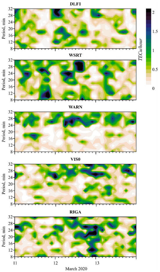
Figure 8.
TEC spectrograms from 11 to 13 March 2020 at the following GNSS stations: DLF1 (51.9° N, 4.4° E), WSRT (52.9° N, 6.6° E), WARN (54.2° N, 12.1° E), VIS0 (57.7° N, 18.4° E), RIGA (56.9° N, 24.1° E).
At the DLF1 and WSRT stations, TEC variations with periods of 10–16 min were observed during the nighttime from 11 March to 12. During the daytime on 12 March, strong TEC variations with periods of 22–30 min were detected at WSRT. Since both of these stations are located on the shore of the North Sea, the spectrum of generated waves in the lower atmosphere may be significantly more intense. At the WARN, VIS0, and RIGA stations, TEC variations with periods of 24–28 min were present throughout the day on 12 March. Notably, at RIGA, spectrograms from the night of 12–13 March reveal variations with periods of 12–16 min. These results clearly indicate that, during the meteorological storm, an increase in TEC variation amplitudes was observed, consistent with the periods of IGWs.
4. Conclusions
This study presents a comprehensive analysis of the impact of Storm Laura, which was observed over Europe and the Baltic Sea on 12 March 2020, on the state of thermosphere–ionosphere system. It is shown that the disturbances in the upper atmosphere and ionosphere observed during this period were a direct consequence of tropospheric processes. The investigation of ionospheric disturbances caused by the meteorological storm was carried out using a combined modeling approach, incorporating the regional AtmoSym model and the global GSM TIP model. This allowed for the consideration of AWs and IGWs generated by tropospheric convective sources and the investigation of wave-induced effects in both the neutral atmosphere and ionosphere.
The simulation results show that, three hours after the activation of the additional heat source, an area of increased temperature exceeding 100 K above the background level formed over the meteorological storm region. This temperature change had a significant impact on the meridional component of the thermospheric wind and TEC variations. For example, meridional wind changes reached 80 m/s compared to a meteorologically quiet day, while TEC variations reached 1 TECu.
A comparison of numerical modeling results with experimental data suggests that atmospheric gravity waves generated in the meteorological storm region and propagating from the troposphere have a significant impact on the thermosphere–ionosphere system. Moreover, the modeling results show reasonable agreement with the experimental data.
Author Contributions
Conceptualization, O.P.B., I.V.K., M.G.G., S.S. and A.V.D.; methodology, O.P.B., F.S.B., Y.A.K. and G.A.Y.; software, O.P.B., F.S.B. and Y.A.K.; validation, O.P.B., A.V.T., F.S.B., Y.A.K. and M.G.G.; formal analysis, A.V.T. and G.A.Y.; investigation, O.P.B., I.V.K., M.G.G. and S.S.; resources, O.P.B., I.V.K. and A.V.D.; data curation, O.P.B., F.S.B., Y.A.K. and G.A.Y.; writing—original draft preparation, O.P.B., F.S.B., Y.A.K., I.V.K., M.G.G., I.G.S. and A.V.D.; writing—review and editing, O.P.B., Y.A.K., I.V.K., M.G.G., S.S. and A.V.D.; visualization, O.P.B. and Y.A.K.; supervision, O.P.B., I.V.K., M.G.G., S.S. and A.V.D.; project administration, O.P.B. and A.V.D.; funding acquisition, O.P.B. and A.V.D. All authors have read and agreed to the published version of the manuscript.
Funding
The research was funded by the grant Russian Science Foundation Nº-23-77-10004, https://rscf.ru/project/23-77-10004/ (accessed 5 June 2025).
Institutional Review Board Statement
Not applicable.
Informed Consent Statement
Not applicable.
Data Availability Statement
The raw data supporting the conclusions of this article will be made available by the authors on request.
Acknowledgments
Solar and geomagnetic indices are available via https://cdaweb.gsfc.nasa.gov/pub/data/omni/, accessed on 30 January 2025. SIMuRG was used for collecting, processing, storage and presentation of GNSS TEC data https://simurg.space/, accessed on 30 January 2025. The authors thank also Artem Padokhin for the MosGIM TEC map data available on https://github.com/gnss-lab/mosgim, accessed on 30 January 2025 and scientific discussion on the interpretation of the obtained results.
Conflicts of Interest
The authors declare no conflicts of interest.
Abbreviations
The following abbreviations are used in this manuscript:
| AWs | Acoustic waves |
| DCB | Differential code bias |
| GNSS | Global navigation satellite system |
| GSM TIP | Global self-consistent model of the thermosphere, ionosphere, and protonosphere |
| IGS | International GNSS service |
| IGWs | Internal gravity waves |
| SIMuRG | System for ionosphere monitoring and research from GNSS |
| TEC | Total electron content |
| TIDs | Traveling ionospheric disturbances |
References
- Laštovička, J. Progress in investigating long-term trends in the mesosphere, thermosphere, and ionosphere. Atmos. Chem. Phys. 2023, 23, 5783–5800. [Google Scholar] [CrossRef]
- Forbes, J.M.; Palo, S.E.; Zhang, X. Variability of the ionosphere. J. Atmos. Sol. Terr. Phys. 2000, 62, 685–693. [Google Scholar] [CrossRef]
- Koucká Knížová, P.; Laštovička, J.; Kouba, D.; Mošna, Z.; Podolská, K.; Potužníková, K.; Šindelářová, T.; Chum, J.; Rusz, J. Ionosphere Influenced from Lower-Lying Atmospheric Regions. Front. Astron. Space Sci. 2021, 8, 651445. [Google Scholar] [CrossRef]
- Chernogor, L.F. A Tropical cyclone or typhoon as an element of the Earth–atmosphere–ionosphere–magnetosphere system: Theory, Simulations, and Observations. Remote Sens. 2023, 15, 4919. [Google Scholar] [CrossRef]
- Yiğit, E.; Medvedev, A.S. Internal wave coupling processes in Earth’s atmosphere. Adv. Space Res. 2015, 55, 983–1003. [Google Scholar] [CrossRef]
- Xiao, Z.; Xiao, S.; Hao, Y.; Zhang, D. Morphological features of ionospheric response to typhoon. J. Geophys. Res. Space Phys. 2007, 112, A04304. [Google Scholar] [CrossRef]
- Snively, J.B. Nonlinear gravity wave forcing as a source of acoustic waves in the mesosphere, thermosphere, and ionosphere. Geophys. Res. Lett. 2017, 44, 12020–12027. [Google Scholar] [CrossRef]
- Sindelarova, T.; Buresova, D.; Chum, J.; Hruska, F. Doppler observations of infrasonic waves of meteorological origin at ionospheric heights. Adv. Space Res. 2009, 43, 1644–1651. [Google Scholar] [CrossRef]
- Hickey, M.P.; Walterscheid, R.L.; Schubert, G. Gravity wave heating and cooling of the thermosphere: Roles of the sensible heat flux and viscous flux of kinetic energy. J. Geophys. Res. 2011, 116, A12326. [Google Scholar] [CrossRef]
- Koucká Knížová, P.; Potužníková, K.; Podolská, K.; Hannawald, P.; Mošna, Z.; Kouba, D.; Chum, J.; Wüst, S.; Bittner, M.; Kerum, J. Multi-instrumental observation of mesoscale tropospheric systems in July 2021 with a potential impact on ionospheric variability in midlatitudes. Front. Astron. Space Sci. 2023, 10, 1197157. [Google Scholar] [CrossRef]
- Golubkov, G.V.; Adamson, S.O.; Borchevkina, O.P.; Wang, P.K.; Dyakov, Y.A.; Efishov, I.I.; Karpov, I.V.; Kurdyaeva, Y.A.; Lukhovitskaya, E.E.; Olkhov, O.A.; et al. Coupling of ionospheric disturbances with dynamic processes in the troposphere. Russ. J. Phys. Chem. B 2022, 16, 508–530. [Google Scholar] [CrossRef]
- Bakhmetieva, N.V.; Zhemyakov, I.N. Vertical plasma motions in the dynamics of the mesosphere and lower thermosphere of the Earth. Russ. J. Phys. Chem. B 2022, 16, 990–1007. [Google Scholar] [CrossRef]
- Bakhmetieva, N.V.; Grigoriev, G.I.; Kalinina, E.E. Propagation of pulses of acoustic gravity waves in the atmosphere and their passage through layers with the given temperature distribution. Russ. J. Phys. Chem. B 2023, 17, 495–502. [Google Scholar] [CrossRef]
- Gann, A.L.S.; Yiğit, E. Ionospheric and Thermospheric Effects of hurricane Grace in 2021 observed by satellites. J. Geophys. Res. Space Phys. 2024, 129, e2024JA032933. [Google Scholar] [CrossRef]
- Koucká Knížová, P.; Podolská, K.; Potužníková, K.; Kouba, D.; Mošna, Z.; Boška, J.; Kozubek, M. Evidence of vertical coupling: Meteorological storm Fabienne on 23 September 2018 and its related effects observed up to the ionosphere. Ann. Geophys. 2020, 38, 73–93. [Google Scholar] [CrossRef]
- Liu, T.; Yu, Z.; Ding, Z.; Nie, W.; Xu, G. Observation of ionospheric gravity waves introduced by thunderstorms in low latitudes China by GNSS. Remote Sens. 2021, 13, 4131. [Google Scholar] [CrossRef]
- Li, K.; Zhang, D.; Zeng, Y.; Tian, Y.; Dai, G.; Liu, Z.; Yang, G.; Sun, S.; Li, G.; Hao, Y.; et al. Revisiting the ionospheric disturbances over low latitude region of China during super typhoon Hato. Space Weather 2024, 22, e2023SW003694. [Google Scholar] [CrossRef]
- Snively, J.B.; Sabatini, R.; Calhoun, D.A.; Heale, C.J.; Inchin, P.A.; Zettergren, M.D. Modeling of acoustic and gravity wave interactions, coupling, and observables above meteorological systems. J. Acoust. Soc. Am. 2022, 151, A161. [Google Scholar] [CrossRef]
- Kshevetskii, S.P.; Kurdyaeva, Y.A.; Gavrilov, N.M. Coupled generation of acoustic and gravity waves by tropospheric heat sources. Russ. J. Phys. Chem. B 2023, 17, 1228–1240. [Google Scholar] [CrossRef]
- Zawdie, K.; Belehaki, A.; Burleigh, M.; Chou, M.Y.; Dhadly, M.S.; Greer, K.; Halford, A.J.; Hickey, D.; Inchin, P.; Kaeppler, S.R.; et al. Impacts of acoustic and gravity waves on the ionosphere. Front. Astron. Space Sci. 2022, 9, 1064152. [Google Scholar] [CrossRef]
- Kurdyaeva, Y.A.; Bessarab, F.S.; Borchevkina, O.P.; Klimenko, M.V. Multimodel study of the influence of atmospheric waves from a tropospheric source on the ionosphere during a geomagnetic storm on 27–29 May 2017. Russ. J. Phys. Chem. B 2024, 18, 852–862. [Google Scholar] [CrossRef]
- Richter, J.H.; Sassi, F.; Garcia, R.R. Toward a Physically Based Gravity Wave Source Parameterization in a General Circulation Model. J. Atmos. Sci. 2010, 67, 136–156. [Google Scholar] [CrossRef]
- Kurdyaeva, Y.A.; Bessarab, F.S.; Borchevkina, O.P.; Klimenko, M.V. Model study of the influence of atmospheric waves on variations of upper atmosphere and ionosphere parameters during a meteorological storm on 29 May 2017. Adv. Space Res. 2024, 74, 2463–2474. [Google Scholar] [CrossRef]
- Gavrilov, N.M.; Kshevetskii, S.P. Three-dimensional numerical simulation of nonlinear acoustic-gravity wave propagation from the troposphere to the thermosphere. Earth Planets Space 2014, 66, 88–95. [Google Scholar] [CrossRef]
- Kurdyaeva, Y.A.; Kshevetskii, S.P.; Gavrilov, N.M.; Golikova, E.V. Well-posedness of a problem of propagation of nonlinear acoustic-gravity waves in the atmosphere generated by surface pressure variations. Numer. Analys. Appl. 2017, 10, 324–338. [Google Scholar] [CrossRef]
- Gavrilov, N.M. The thermal effect of internal gravity waves in the upper atmosphere. Izv. Atmos. Ocean. Phys. 1974, 10, 45–46. [Google Scholar]
- Namgaladze, A.A.; Korenkov, Y.N.; Klimenko, V.V.; Karpov, I.V.; Surotkin, V.A.; Naumova, N.M. Numerical modelling of the thermosphere-ionosphere-protonosphere system. J. Atmos. Terr. Phys. 1991, 53, 1113–1124. [Google Scholar] [CrossRef]
- Klimenko, M.V.; Klimenko, V.V.; Bryukhanov, V.V. Numerical simulation of the electric field and zonal current in the Earth’s ionosphere: The dynamo field and equatorial electrojet. Geomagn. Aeron. 2006, 46, 457–466. [Google Scholar] [CrossRef]
- Afraimovich, E.L.; Astafyeva, E.I.; Demyanov, V.V.; Edemskiy, I.K.; Gavrilyuk, N.S.; Ishin, A.B.; Kosogorov, E.A.; Leonovich, L.A.; Lesyuta, O.S.; Palamartchouk, K.S.; et al. A review of GPS/GLONASS studies of the ionospheric response to natural and anthropogenic processes and phenomena. J. Space Weather Space Clim. 2013, 3, A27. [Google Scholar] [CrossRef]
- Yasyukevich, Y.V.; Kiselev, A.V.; Zhivetiev, I.V.; Edemskiy, I.K.; Syrovatskii, S.V.; Maletckii, B.M.; Vesnin, A.M. SIMuRG: System for ionosphere monitoring and research from GNSS. GPS Solut. 2020, 24, 69. [Google Scholar] [CrossRef]
- Schaer, S. Mapping and Predicting the Earth’s Ionosphere Using the Global Positioning System. Ph.D. Thesis, University of Bern, Bern, Switzerland, 1999; p. 205. [Google Scholar]
- Padokhin, A.M.; Andreeva, E.S.; Nazarenko, M.O.; Kalashnikova, S.A. Phase-difference approach for GNSS global ionospheric total electron content mapping. Radiophys. Quantum Electron. 2022, 65, 481–495. [Google Scholar] [CrossRef]
- Shagimuratov, I.I.; Chernyak, Y.V.; Zakharenkova, I.E.; Yakimova, G.A. Use of total electron content maps for analysis of spatial-temporal structures of the ionosphere. Russ. J. Phys. Chem. B 2013, 7, 656–662. [Google Scholar] [CrossRef]
- Troshichev, O.A.; Andrezen, V.G. The relationship between interplanetary quantities and magnetic activity in the southern polar cap. Planet. Space Sci. 1985, 33, 415–419. [Google Scholar] [CrossRef]
- Stauning, P. A new index for the interplanetary merging electric field and geomagnetic activity: Application of the unified polar cap indices. Space Weather 2007, 5, S09001. [Google Scholar] [CrossRef]
- Rishbeth, H. How the Thermospheric Circulation Affects the Ionospheric F2-Layer. J. Atmos. Sol.-Terr. Phys. 1998, 60, 1385–1402. [Google Scholar] [CrossRef]
- Borchevkina, O.; Karpov, I.; Karpov, M. Meteorological storm influence on the ionosphere parameters. Atmosphere 2020, 11, 1017. [Google Scholar] [CrossRef]
- Yasyukevich, Y.V.; Mylnikova, A.A.; Kunitsyn, V.E.; Padokhin, A.M. Influence of GPS/GLONASS differential code biases on the determination accuracy of the absolute total electron content in the ionosphere. Geomagn. Aeron. 2015, 55, 763–769. [Google Scholar] [CrossRef]
- Yasyukevich, Y.V.; Mylnikova, A.A.; Polyakova, A.S. Estimating the total electron content absolute value from the GPS/GLONASS data. Results Phys. 2015, 5, 32–33. [Google Scholar] [CrossRef]
- Mylnikova, A.A.; Yasyukevich, Y.V.; Kunitsyn, V.E.; Padokhin, A.M. Variability of GPS/GLONASS differential code biases. Results Phys. 2015, 5, 9–10. [Google Scholar] [CrossRef]
- Lomb, N.R. Least-squares frequency analysis of unequally spaced data. Astrophys. Space Sci. 1976, 39, 447–462. [Google Scholar] [CrossRef]
- Scott, C.J.; Stamper, R.; Rishbeth, H. Long-term changes in thermospheric composition inferred from a spectral analysis of ionospheric F-region data. Ann. Geophys. 2014, 32, 113–119. [Google Scholar] [CrossRef][Green Version]
- Burkholder, B.L.; Cuellar, R.; Nykyri, K.; Ma, X.; Debchoudhury, S. A regional classification of time spectral amplitudes in total electron content: Southeastern United States during solar cycle 24. Front. Astron. Space Sci. 2022, 9, 1040082. [Google Scholar] [CrossRef]
Disclaimer/Publisher’s Note: The statements, opinions and data contained in all publications are solely those of the individual author(s) and contributor(s) and not of MDPI and/or the editor(s). MDPI and/or the editor(s) disclaim responsibility for any injury to people or property resulting from any ideas, methods, instructions or products referred to in the content. |
© 2025 by the authors. Licensee MDPI, Basel, Switzerland. This article is an open access article distributed under the terms and conditions of the Creative Commons Attribution (CC BY) license (https://creativecommons.org/licenses/by/4.0/).