RANS and LES Simulations of Localized Pollutant Dispersion Around High-Rise Buildings Under Varying Temperature Stratifications

Abstract

This research investigates the influence of buildings on the flow pattern and pollutant spread under different temperature stratification scenarios. Using Reynolds-averaged Navier–Stokes (RANS) equations alongside the large eddy simulation (LES) model, the findings were validated through comparisons with wind tunnel experiments. Results indicate that the return zone length on the leeward side of the building is the longest, around 1.75 times the building height (H) when the Richardson number (Ri_b) is 0.08. This return zone length reduces to approximately 1.4 H when Ri_b is 0.0 and further decreases to 1.25 H with a Ri_b of −0.1. Pollutant dispersion is similarly affected by the flow field, which aligns with these trends. The studied models revealed that LES proved the most accurate, closely matching wind tunnel results across all temperature stratification levels, while RANS overestimated values at building height (z/H = 1.0) and around the building (x/H < 0.625). To balance computational efficiency with prediction accuracy, a hybrid method integrating LES and RANS is recommended.

1. Introduction

The rapid expansion of urban areas and population growth in recent years have driven the development of numerous high-rise buildings to alleviate urban land shortages. These tall structures can significantly alter the surrounding flow field and affect pollutant dispersion, raising concerns about accurately and promptly predicting these effects [1,2]. While a substantial amount of research has focused on neutral stratification conditions, comparatively fewer studies have explored how different temperature stratifications influence these dynamics.

Kanda and Yamao [3] carried out wind tunnel experiments to explore the influence of temperature stratifications on the spread of point source pollution in urban areas. By manipulating the air temperature and the temperature of the base plate within the experimental section, they found that temperature stratifications play a crucial role in influencing pollutant dispersion. Another study investigated the impact of stable and unstable stratifications on turbulent motion using wind tunnel experiments, concluding that buoyancy dampens turbulence under stable conditions. Yassin [4] explored the impact of temperature stratification on flow pattern and pollutant spread in the wake of urban buildings, noting that unstable stratification intensifies longitudinal turbulence in its wake, leading to reduced pollutant concentration, while stable stratification results in higher pollutant concentration. Similarly, Marucci and Carpentieri [5,6] conducted wind tunnel studies to analyze the impact of temperature stratifications on the flow pattern and pollutant diffusion around arrays of buildings. Their research revealed that temperature stratification had a stronger influence on pollutant dispersion in the vertical plane compared to the horizontal. Specifically, pollutant concentrations under stable stratification were found to be twice as high as those under neutral stratification, whereas under unstable conditions, pollutant concentrations were reduced to about one-third of those in neutral stratification. Yan and Li [7] used wind tunnel experiments to investigate the interference effects between double supertall buildings with complex external shapes.

Recently, computational fluid dynamics (CFD) has become the leading approach for modeling pollutant dispersion in urban settings. The most widely used CFD models include the RANS equations and LES. Zhou et al. [8] used the RANS method and found that the effect of buildings on the average temperature distribution in the downstream area is more pronounced when the stability is low. Jeong and Kim [9] investigated the effect of isolated buildings on near-field pollutant dispersion under different atmospheric stabilization conditions using the RANS method and found that the pollutant plume from the rear of the building spreads laterally under stabilized conditions, which leads to higher near-surface pollutant concentrations than under unsteady and neutral conditions. Wang et al. [10] investigated the relationship between the gap layout of the building-to-street length ratio and air quality by the CFD method, and the results showed that for parallel streets, the air quality improved in a linear trend as the gap width increased. However, for vertical streets, the relationship between gap width and air quality is not linear. Yassin et al. [11] investigated the flow field and gas diffusion around a building under three different degrees of stability by using the k-e turbulence model and found that pollutant concentrations increased under stable stratification and decreased under unstable stratification. Tominaga and Stathopoulos [12] used the RANS model to simulate the spread of light, medium, and heavy gases around an isolated building, later comparing the simulation outcomes with wind tunnel experiment data. They observed that the RANS model underestimates light gas dispersion while overestimating the spread of heavier gases. Guo et al. [13,14] explored the impact of buildings on the flow pattern and pollutant distribution under various temperature stratifications using RANS. They found that as the Ri_b (Ri_b is bulk Richardson number, its definition is given in Equation (20)) increased, the static point on the windward side of the building shifted upward, reducing the vertical range of pollutant dispersion while concentrations gradually increased. Madalozzo et al. [15] focused on the impact of street valley width on flow and pollutant dispersion. Their results showed that narrower valleys (with a height-to-width ratio of H/W = 0.5) experienced lower wind speeds and higher pollutant concentrations, whereas wider valleys (H/W = 2.0) displayed increased wind speeds and reduced pollutant levels. Ehsan et al. [16] investigated the effect of ambient wind speed on the variation in the maximum pollution concentration by means of a detached eddy simulation and found that critical zones were generally formed behind the walls of upstream buildings, near the walls upstream of the highway, and in front of the walls of downstream buildings.

With advances in computational power, the LES method has been increasingly employed in pollutant dispersion studies. The LES model has a wide range of applications in the study of vortices on the leeward side of buildings, especially for capturing the complex dynamic behavior of fluids as well as vortex generation, shedding, and evolution processes [17,18,19,20]. Chao et al. [21,22] indicated that LES models are often used to evaluate the impact of buildings on the surrounding wind field and pollutant dispersion. Chatzimichailidis et al. [23] investigated the wind field distribution and pollutant dispersion characteristics within an ideal two-dimensional street valley and analyzed the LES results qualitatively and quantitatively in various aspects. Xie et al. [24] employed the LES method to analyze the effects of temperature stratifications on pollutant spread in urban settings, observing that under unstable stratification, pollutants diffused more extensively in the vertical direction compared to neutral stratification. Jiang and Yoshie [25] applied the LES method to investigate microscale pollutant dispersion from a 3D urban street model in unstable stratification conditions, verifying the results with wind tunnel tests. They found that the LES predictions for mean velocity and fluctuations closely matched those observed experimentally. More recently, Guo et al. [26] used the LES method to study the influence of buildings on the surrounding flow field and pollutant dispersion under various stable stratifications, identifying a critical Ri_b range between 0.22 and 0.3.

Calculations indicate that LES generally demands 13.2 times more computational time than RANS simulations under similar conditions [27]. Numerous studies have examined the differences between the RANS approach and the LES method, comparing prediction accuracy [28,29,30], assessing turbulence quality [31,32], analyzing temperature stratification effects [33], and evaluating computational parameters [34,35]. Blocken [36] demonstrated the advantages of the LES method by comparing flow patterns around a building under various conditions, showing its capacity to simulate flow instability more effectively than RANS. Ishihara et al. [37] used modified k-ε and LES turbulence models to study flow fields within uniform cubic arrays of different densities and in an actual urban setting. They found that the LES method accurately captured the flow field around buildings in both cases, while the k-ε model showed limited accuracy for real urban flow structures. Additionally, Tominaga and Stathopoulos [38] simulated pollutant dispersion around a building using RANS and LES. Their comparison revealed that RANS generally overestimated pollutant concentration, while LES provided more accurate results for horizontal pollutant spread.

While several studies have compared the RANS and LES methods, most have focused on neutral stratification, with limited research exploring the performance of the two methods under varying temperature stratifications. To address this gap, the present study investigates the effects of stable stratification (Ri_b = 0.08), neutral stratification (Ri_b = 0.0), and unstable stratification (Ri_b = −0.1) on flow patterns and pollutant dispersion around a high-rise building. To this end, the RANS and LES methods are applied, with their performance validated through wind tunnel experiments. Additionally, a detailed comparison between RANS and LES results is performed to evaluate the accuracy of each model in simulating atmospheric conditions.

2. Research Methodology

The distribution of the temperature of the quiescent atmosphere in the vertical direction is usually referred to as the atmospheric temperature stratifications. The decrease in air temperature along increasing altitude is called unstable stratification. The increase in air temperature with increasing altitude is known as stable stratification. Temperature that does not vary with altitude is called neutral stratification.

STAR-CD is a commercially available software package for CFD. Its core algorithms are based on the finite volume method, which supports unstructured meshing to handle complex geometries and provides a variety of differential formats and turbulence models. In this research, STAR-CD serves as the computational platform, utilizing both the RANS and LES methods for simulations. Given the relatively low airflow velocity and negligible changes in gas density, the gas can be considered an incompressible fluid. The governing equations can be expressed as

$$\nabla ·\left(\rho \overrightarrow{U}\right)=0$$

(1)

$$\nabla ·\left(\rho \overrightarrow{U}\overrightarrow{U}\right)=-\nabla p+\nabla ·\tau +S_B$$

(2)

$$\nabla ·\left(\rho \overrightarrow{U}{c}_{p}T\right)=\nabla ·\left(k_T\nabla T\right)+S_r$$

(3)

$$\nabla ·\left(\rho \overrightarrow{U}{y}_m\right)=\nabla ·D_m\nabla \left(y_m\right)+S_m m=1,\cdots ,n$$

(4)

In these equations, $\rho$ represents the density, $\overrightarrow{U}$ is the velocity vector, p denotes pressure, and $\tau$ refers to the viscous stress tensor. The specific heat capacity at constant pressure is indicated by c_p, while k_T signifies effective thermal conductivity. The mass fraction is represented by y_m, and D_m is the effective diffusion coefficient for the substance component m. Temperature is denoted by T, and S_B, S_T, and S_m are generalized source terms, which represent the sum of all the other terms in the unsteady term, the convection term, and the diffusion term that cannot be included in the governing equations.

2.1. RANS Method

The k–ε high-Reynolds turbulence model [39] is employed in this study for simulations using the RANS method. The equations governing the k–ε high-Reynolds turbulence model are expressed as follows:

$${\displaystyle \frac{\partial }{\partial t}}(k)+{\displaystyle \frac{\partial }{\partial x_j}}[u_{j}k-(\mu +{\displaystyle \frac{{\mu }_t}{{\sigma }_k}}){\displaystyle \frac{\partial k}{\partial x_j}}]={\mu }_t(P_T+P_B)-\epsilon -{\displaystyle \frac{2}{3}}({\mu }_t{\displaystyle \frac{\partial u_i}{\partial x_i}}+k){\displaystyle \frac{\partial u_i}{\partial x_i}}$$

(5)

$${\displaystyle \frac{\partial }{\partial t}}(\epsilon )+{\displaystyle \frac{\partial }{\partial x_j}}[u_j\epsilon -(\mu +{\displaystyle \frac{{\mu }_t}{{\sigma }_{\epsilon }}}){\displaystyle \frac{\partial \epsilon }{\partial x_j}}]=A+B$$

(6)

$$P_T=S_{ij}{\displaystyle \frac{\partial u_i}{\partial x_j}}$$

(7)

$$P_B=-{\displaystyle \frac{g_i}{{\sigma }_{h,t}}}{\displaystyle \frac{\partial T}{\partial x_j}}$$

(8)

$$A=C_{\epsilon 1}{\displaystyle \frac{\epsilon }{k}}[{\mu }_t{P}_T-{\displaystyle \frac{2}{3}}({\mu }_t{\displaystyle \frac{\partial u_i}{\partial x_i}}+k){\displaystyle \frac{\partial u_i}{\partial x_i}}]$$

(9)

$$B=C_{\epsilon 3}{\displaystyle \frac{\epsilon }{k}}{\mu }_t{P}_B-C_{\epsilon 2}{\displaystyle \frac{{\epsilon }^2}{k}}+C_{\epsilon 4}\epsilon {\displaystyle \frac{\partial u_i}{\partial x_i}}+C_{\epsilon 1}{\displaystyle \frac{\epsilon }{k}}{\mu }_t{P}_{NL}$$

(10)

$$P_{NL}=-{\displaystyle \frac{\rho }{{\mu }_t}}\overline{{u_i}^{\prime }{u_j}^{\prime }}{\displaystyle \frac{\partial u_i}{\partial x_j}}-[P-{\displaystyle \frac{2}{3}}({\displaystyle \frac{\partial u_i}{\partial x_i}}+{\displaystyle \frac{\rho k}{{\mu }_t}}){\displaystyle \frac{\partial u_i}{\partial x_i}}]$$

(11)

where k represents the turbulent kinetic energy. $\epsilon$ denotes the turbulent dissipation rate. $\mu$ refers to the dynamic viscosity. ${\mu }_t$ indicates the turbulent viscosity. $S_{ij}$ represents the mean velocity strain rate. P_T corresponds to turbulent stress. P_B signifies the turbulent kinetic energy generated by buoyancy.$P_{NL}=0$ is the linear model, ${\sigma }_k$, ${\sigma }_{\epsilon }$, and ${\sigma }_h$ are the turbulent Planck numbers, and ${\sigma }_m$ is the turbulent Schmidt number. $C_{\epsilon 1}$, $C_{\epsilon 2}$, $C_{\epsilon 3}$, and $C_{\epsilon 4}$ are the empirical constants. The turbulence model constants are shown in

Table 1. The turbulence model constants.

${\mathit{C}}_{\mathit{\mu }}$	${\mathit{\sigma }}_{\mathit{k}}$	${\mathit{\sigma }}_{\mathit{\epsilon }}$	${\mathit{\sigma }}_{\mathit{h}}$	${\mathit{\sigma }}_{\mathit{m}}$	${\mathit{C}}_{\mathit{\epsilon }1}$	${\mathit{C}}_{\mathit{\epsilon }2}$	${\mathit{C}}_{\mathit{\epsilon }3}$	${\mathit{C}}_{\mathit{\epsilon }4}$	$\mathit{\kappa }$	$\mathit{E}$
0.09	1.0	1.22	0.9	0.9	1.44	1.92	1.44	−0.33	0.419	9.0

.

2.2. LES Method

The LES method utilizes the Smagorinsky subgrid model, which is based on the principle of Boussinesq vortex viscosity [40,41]. In this context, the terms for subgrid stress, scalar flux, and enthalpy flux are defined as follows:

$${\tau }_{ij}^{SGS}=(\overline{u_i{u}_j}-{\overline{u}}_i{\overline{u}}_j)$$

(12)

$$\rho (\overline{u_{i}h}-{\overline{u}}_i\overline{h})=-{\displaystyle \frac{{\mu }_{SGS}{c}_p}{{\mathrm{Pr}}_{SGS}}}{\displaystyle \frac{\partial \overline{\theta }}{\partial x_i}}$$

(13)

$$J_j^{SGS}=(\overline{u_{j}c}-{\overline{u}}_j\overline{c})$$

(14)

where ${\mu }_{SGS}$ and $P{r}_{SGS}$ are the subgrid viscosity and Prandtl number, respectively. Since the building is surrounded by incompressible fluid, the governing equations can be solved using the ideal gas equation with a computational density of

$$\rho ={\displaystyle \frac{p_{op}}{(R/M_w)\theta }}$$

(15)

where temperature θ is obtained from the energy equation, R is the universal gas constant, M_w is the molecular weight of air, and p_op is the operating pressure. According to the ideal gas law, changes in density are influenced exclusively by changes in temperature.

The subgrid-scale is given below.

$${\mu }_{SGS}=l_0^2·S$$

(16)

$$S^2={\displaystyle \frac{1}{2}}{({\displaystyle \frac{\partial {\overline{u}}_i}{\partial x_j}}+{\displaystyle \frac{\partial {\overline{u}}_j}{\partial x_j}})}^2$$

(17)

where l₀ is the mixing-length, $l_0=C_S△$, C_S is the proportionality coefficient, and $△$ is the geometric mean scale of the grid, $△={\left(△x△y△z\right)}^{1/3}$.

The LES method differs from the k-ε high-Reynolds turbulence model by incorporating a wall-adapting local eddy-viscosity (WALE) model. This feature enables the LES method to effectively capture turbulence scales near the wall without requiring a damping function. The WALE model has proven to be effective in accurately predicting the flow and concentration fields near the building [42,43,44]. In contrast to the RANS method, the LES method is often used for near-wall turbulence modeling under different stratifications.

3. Numerical Techniques

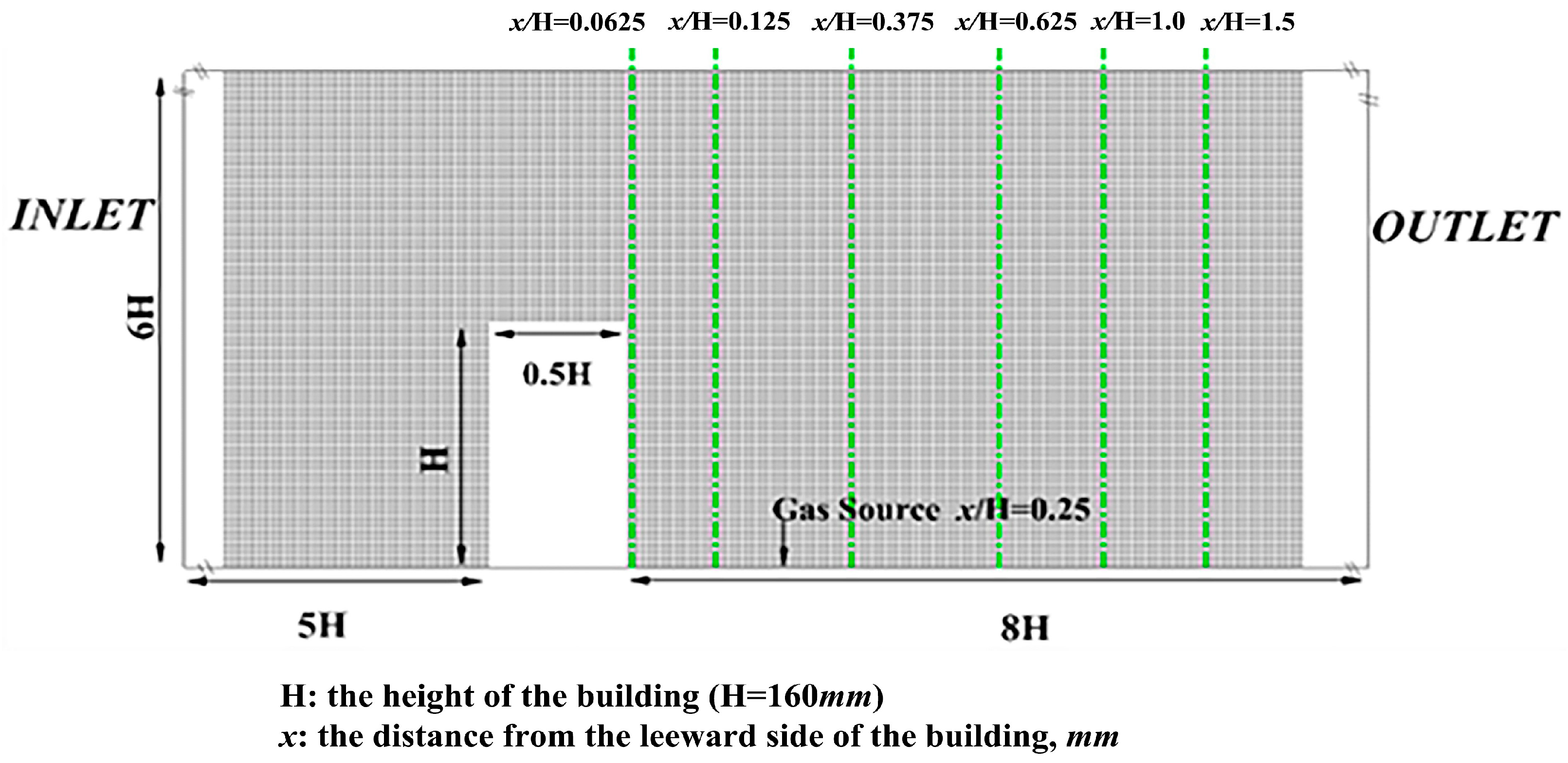
3.1. Numerical Model

The wind tunnel experimental data used in this study were sourced from the Architectural Institute of Japan (AIJ) [45]. The experiments were conducted in a temperature stratification wind tunnel at the Tokyo Institute of Technology. Figure 1 schematically presents the computational domain ($12.75\mathrm{H}(\overrightarrow{x})\times 6.875\mathrm{H}(\overrightarrow{y})\times 5.625\mathrm{H}(\overrightarrow{z})$) along with the placement of the sampling points for this investigation. The model building is cubic, measuring 80 mm in length (L), 80 mm in width (W), and 160 mm in height (H). x indicates the distance from the leeward side of the building. The contamination source is positioned 40 mm from the leeward side of the building, and the tracer gas (C₂H₄) is emitted at a flow rate of q = 9.17 × 10⁻⁶ m³/s through an opening with a diameter of 5 mm.

3.2. Parameter Setting

In this research, the numerical simulations are performed following the incoming boundary conditions defined by the wind tunnel experiments. The wind speed contours are generated according to the exponential law, as expressed in Equation (18). To obtain temperature contours reflecting different stratifications, the temperature gradient is adjusted accordingly. The SIMPLE algorithm is utilized to ensure quick convergence and accuracy of numerical results. A second-order central difference scheme [46,47] is employed for the spatial discretization of momentum, concentration, energy, and pressure. Both the ground and upper boundaries are modeled as no-slip walls, with a ground roughness (z₀) of 0.001 m.

Table 2. Setting of the main parameters.

Stratifications	Rib	TH (K)	Tf (K)	△T (K)	uH(m/s)	Time Step (s)	Sampled Time (s)
Unstable	−0.1	284.3	318.3	−34.0	1.37	0.0015	15.0–75.0
Neutral	0.0	294.35	294.35	0.0	1.4	0.0014	14.0–70.0
Stable	0.08	322.4	291.0	56.0	1.37	0.0015	15.0–75.0

summarizes the key parameters from the wind tunnel experiments and the corresponding numerical simulations. The larger value of △T in Table 2 is to make the influence of different temperature stratifications on the flow field around the building and the diffusion of pollutants more obvious.

$$u=u_H{({\displaystyle \frac{z}{z_H}})}^n$$

(18)

where u is the velocity at height z and n is the stability parameter n = 0.27.

In atmospheric research, Re and Ri_b are commonly used to evaluate airflow characteristics and atmospheric stability. These dimensionless parameters are defined in the form below.

$$Re={\displaystyle \frac{u_H\cdot H}{v}}$$

(19)

$${\mathit{Ri}}_b={\displaystyle \frac{\mathit{gH}(T_H-T_f)}{T_f{u}_H^2}}$$

(20)

where u_H represents the average flow velocity at the building height (H) and v is the kinematic viscosity coefficient. T_H indicates the temperature of the incoming atmosphere at the top of the building, while T_f signifies the temperature at the ground level. Additionally, g = 9.8 m/s² represents the gravitational acceleration.

3.3. Mesh Independence Analysis

This study utilizes a hexahedral mesh to create three distinct mesh discretization schemes, each defined by varying mesh sizes and total mesh counts. The hexahedral mesh is advantageous due to its ability to maintain a low mesh count and facilitate rapid convergence [48]. The three schemes are categorized as follows: a rough mesh (4 mm mesh, 2.1 × 10⁶ meshes); a basic mesh (2 mm mesh, 4.2 × 10⁶ meshes); and a fine mesh (1 mm mesh, 8.4 × 10⁶ meshes). The RANS and LES methods use the same mesh discretization scheme to allow for a clear comparison of the differences between the two methods. The simulation outcomes for these three configurations are compared and analyzed under a condition of Ri_b = 0.08. Figure 2 presents a comparison of the normalized longitudinal mean velocity (u/u_H), normalized vertical mean velocity (w/u_H), and normalized mean concentration (c/c₀) at different heights at the position x/H = 0.375 downstream of the building. The results indicate a similar trend across the three grid simulations, with the basic and fine grids showing a closer alignment, while the rough grid reveals a notable deviation at the building height. Given the need for accurate simulation results and the goal of minimizing simulation time, the basic grid is selected for the numerical simulation in this research.

4. Results and Discussion

This study employs numerical simulations using the LES and RANS methods to explore the impact of building on the surrounding flow pattern and pollutant dispersion across different temperature stratifications. Furthermore, the research aims to evaluate the results obtained from wind tunnel experiments concerning the findings from the numerical simulations.

4.1. Velocity Field

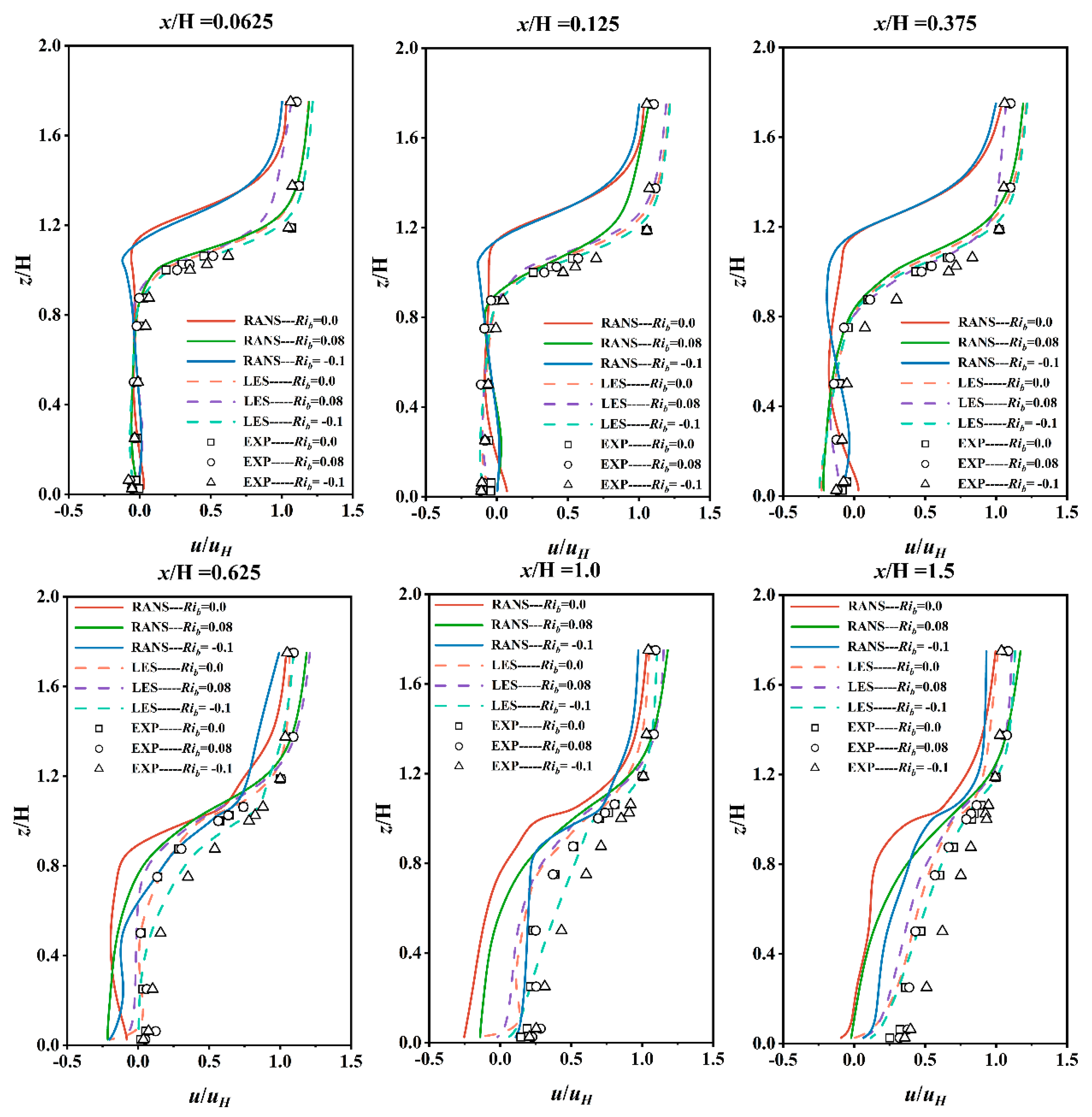
4.1.1. Mean Longitudinal Velocity

Figure 3 compares u/u_H curves recorded during wind tunnel experiments with results from LES and RANS methods across different Ri_b conditions at various locations on the leeward side of the building. The figure highlights the existence of a recirculation zone on the leeward side, characterized by a significant decrease in u/u_H as one approaches this area. Notably, the velocity loss at Ri_b = 0.08 is greater than at Ri_b = 0.0 and Ri_b = −0.1, indicating that mechanical disturbances exert a predominant influence on the leeward side, while the effects of temperature stratification are relatively minor on the flow field structure. As the distance downwind increases, the airflow becomes increasingly homogeneous, with wind speeds gradually returning to their original state. This recovery is slower at Ri_b = 0.08, followed by Ri_b = 0.0, and it is most rapid at Ri_b = −0.1. For distances where x/H ≤ 0.375, the trends for Ri_b = 0.0 and Ri_b = −0.1 closely align, with the strongest airflow reaction occurring at z/H = 0.25, where the minimum value of u/u_H is −0.17. In contrast, at Ri_b = 0.08, the most pronounced airflow reaction occurs at z/H = 0.8, with a minimum value of u/u_H reaching −0.22.

Figure 3 demonstrates that the numerical simulation provides a more accurate estimation of the longitudinal mean velocity distribution on the leeward side of the building. The LES results align closely with the wind tunnel tests across various Ri_b conditions. Specifically, at Ri_b = 0.08, the RANS simulation results for x/H < 0.125 show a strong agreement with the experimental findings; however, discrepancies arise in all other locations. At Ri_b values of 0.0 and −0.1, deviations from the experimental results are noted across all locations. Significant differences in results are particularly evident at the building height (z/H = 1.0) across the various Rib configurations. This divergence is primarily attributed to the tendency of the RANS method to overestimate the height and the extent of the recirculation zone on the leeward side of the building [49]. Consequently, this overestimation leads to u/u_H values that exceed those predicted by the LES model.

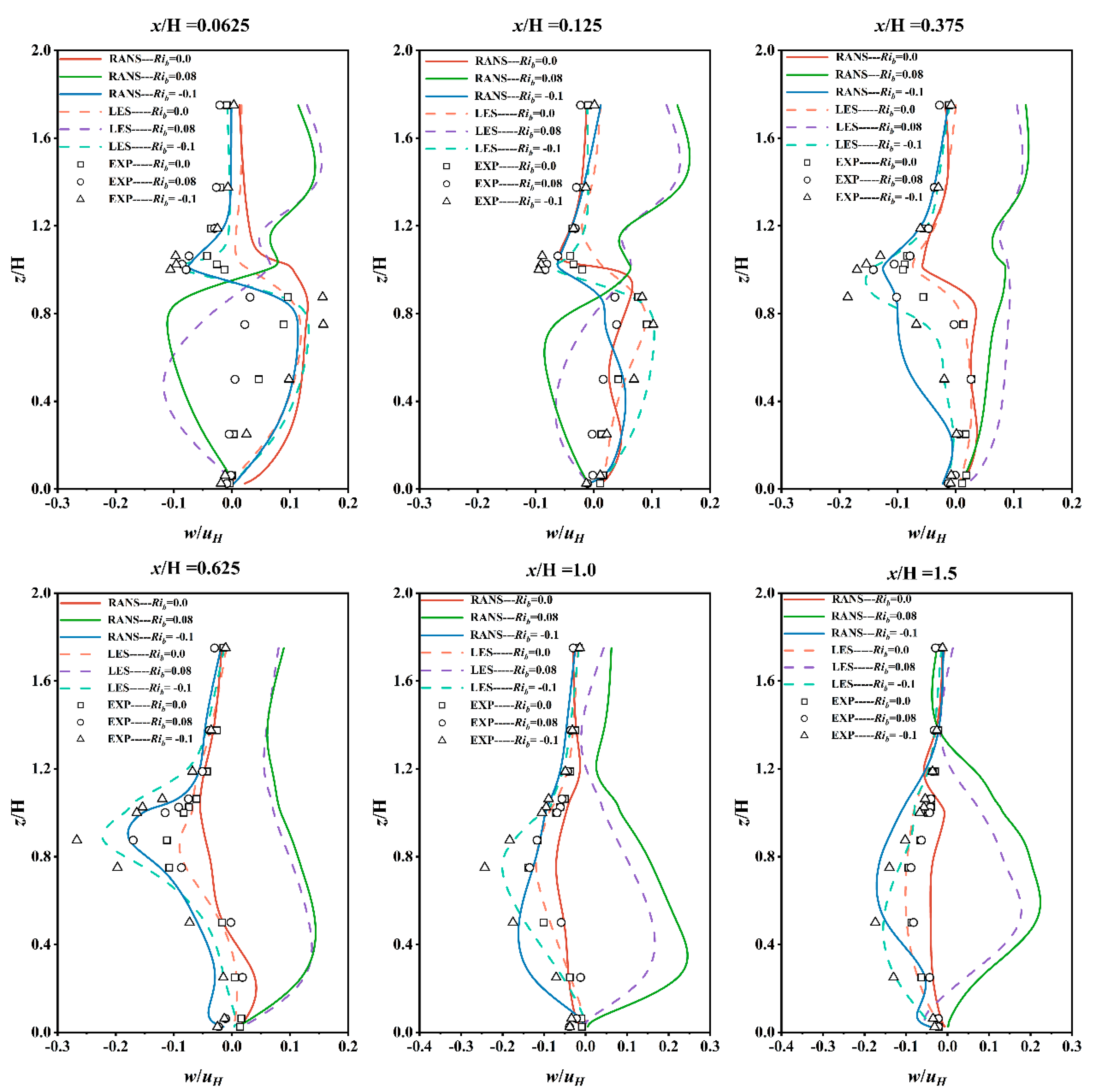
4.1.2. Mean Vertical Velocity

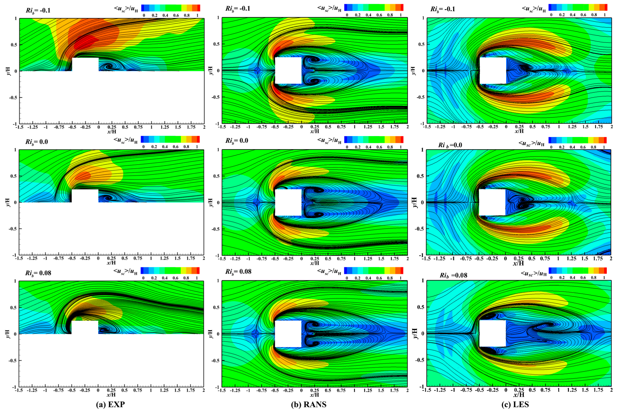
Figure 4 compares w/u_H curves between the wind tunnel experiments and numerical results at different locations on the leeward side of the building for various Ri_b conditions. The data indicate that the variations for Ri_b values of 0.0 and −0.1 are similar, whereas the changes are more pronounced at Ri_b = 0.08. Notably, the w/u_H values for Ri_b = 0.0 are generally close to zero in the vertical direction. In the proximity range (x/H ≤ 0.625), the differences in w/u_H values across the different temperature stratifications are negligible due to the influence of turbulence around the building and within the recirculation zone. However, beyond x/H > 0.625, the effects of the temperature laminar junction begin to appear. For Ri_b values of 0.0 and −0.1, the maximum w/u_H occurs at z/H = 0.8, while at Ri_b = 0.08, the peak occurs at z/H = 0.4. This variation is primarily attributed to stable laminar junction conditions, buoyant forces, and a reduction in turbulent activity. The airflow exhibits a downward direction when the air temperature is higher than that at the ground level, a phenomenon observed in [50] in the authors’ wind tunnel experiments.

Figure 4 shows that the results from the LES method under the three Ri_b conditions closely match the findings from the wind tunnel experiments. In contrast, the RANS method produces substantial errors at heights below the building (z/H ≤ 1.0). However, the discrepancies are reduced above the building height. It is worth noting that this discrepancy primarily originates from limitations of the RANS method in accurately simulating the wind shear effects of the airflow around the building [49].

4.1.3. Flow Pattern

Figure 5 and Figure 6 illustrate the flow pattern through a normalized mean velocity cloud map (<u_sc>/u_H) for vertical (y/H = 0.0) and horizontal (z/H = 0.05) profiles around the building across different temperature stratifications, where <u_sc> represents the mean resultant velocity, as assessed by three different methods. Figure 5 demonstrates that the formation of a vortex on the leeward side of the building is influenced by temperature stratifications. These stratifications affect the characteristics of the vortex, including its size and position. Specifically, the vortex center identified in the wind tunnel experiments is located at x/H = 0.3, while the RANS method places it at x/H = 0.4. The stationary point on the windward side remains consistent at z/H = 0.75 across both methods. However, the vortex center from the LES method occurs at x/H = 0.2, with the stationary point on the windward side also at z/H = 0.75, indicating a distinct top return zone at the apex of the building. The LES results provide a more accurate representation of the flow pattern around the building compared to the wind tunnel experiments. The main discrepancy between the experimental results and the numerical simulations lies in the placement of the reattachment point on the leeward side, which appears near x/H = 0.5 in the experiments. For Ri_b = −0.1, the RANS and LES methods yield reattachment points at x/H = 1.25 and x/H = 1.2, respectively. For Ri_b = 0.0, the reattachment points are at x/H = 1.5 for the RANS method and x/H = 1.25 for the LES method. Similarly, for Ri_b = 0.08, the RANS and LES methods place the reattachment points at x/H = 1.6 and x/H = 1.5, respectively. Notably, the CFD results show that the reattachment points are located further from the leeward side of the building compared to those observed in the wind tunnel experiments.

As illustrated in Figure 5c, the vortex locations on the leeward side of the building across different temperature stratifications are centered around x/H = 0.2. For a Ri_b of 0.08, the vortex exhibits the smallest size and is positioned at the lowest height, approximately z/H = 0.15. In this case, the furthest reattachment point on the leeward side is around x/H = 1.5. Conversely, at Ri_b = 0.0, the vortex is notably larger, with its height at approximately z/H = 0.4, and the corresponding reattachment point on the leeward side is roughly at x/H = 1.25. When Ri_b = −0.1, the vortex size decreases compared to the scenario with Ri_b = 0.0, with a height around z/H = 0.3, and the leeward-side reattachment point is located at about x/H = 1.15. Analyzing the <u_sc>/u_H contour reveals that the maximum value of <u_sc>/u_H on the leeward side of the building occurs at Ri_b = −0.1, while the minimum value is observed at Ri_b = 0.08.

Figure 6 shows that the flow field is significantly altered due to the presence of the building. The momentum along the wind axis on the windward side is redirected into both horizontal and vertical components, resulting in a return flow that creates a double-vortex return, characterized as a horseshoe-shaped vortex, on the leeward side of the structure. According to the RANS method, the separation point on the windward side is located at approximately x/H = −0.8, with the center of the horseshoe vortex positioned around x/H = 0.3. Conversely, the LES method indicates that the separation point is closer to the building, approximately at x/H = −0.6. When comparing the two methods, the LES model demonstrates a lower <u_sc>/u_H value on the windward side and provides a more accurate representation of the return zone on both sides of the building than the RANS method.

Figure 6c demonstrates that when Ri_b = 0.08, the length of the return area on the leeward side of the building is the largest, measuring approximately 1.75 H. In this scenario, the center of the vortex on the leeward side is positioned farthest from the building, with a broader variation range of the flow lines, approximately ±0.6 in the y/H dimension. In contrast, for Ri_b values of 0.0 and −0.1, the range of flow line variation is narrower, around ±0.5 in width. This difference is primarily attributed to the conditions of atmospheric stability: under unstable stratification, the temperature distribution is uneven, leading to significant changes in air pressure and density, which results in heightened turbulence. Conversely, stable stratification results in smaller changes in air density and pressure, resulting in weaker turbulent movements.

4.2. Concentration Field

Figure 7 compares <c>/c₀ curves between the wind tunnel experiments and the simulations from the LES and RANS methods at various locations on the leeward side of the building, considering different Ri_b conditions. <c> represents the average concentration, and c₀ is the reference gas concentration $c_0=c_{gas}·q/u_H{H}^2$, where q denotes the gas flow rate. It is observed that the discrepancies between the RANS and LES methods are primarily evident near the leeward side of the building (for x/H < 0.625). The pollutant concentration decreases progressively with increasing downwind distance. This phenomenon may be attributed to the formation of a return zone on the leeward side that facilitates the accumulation of pollutants in that vicinity. For all three temperature stratification conditions, the highest <c>/c₀ values occur at x/H = 0.125, reaching a peak of 503.36. When z/H > 1.0, the concentration value for Ri_b = −0.1 is the highest, while for Ri_b = 0.08, it is the lowest. In contrast, for z/H ≤ 1.0, the increase in <c>/c₀ is most pronounced for Ri_b = 0.08, whereas Ri_b = −0.1 exhibits the smallest values as height decreases. This variation is primarily due to the stable lamination, which hinders the vertical diffusion of pollutants, causing them to accumulate at the ground level due to buoyancy effects. Beyond x/H ≥ 0.625, the effects of temperature stratifications on pollutant diffusion become more apparent; however, at locations near the building (for x/H < 0.625), the changes in <c>/c₀ are predominantly driven by disturbances caused by the building.

As illustrated in Figure 7, the numerical methods can effectively estimate the distribution of pollutant concentrations on the leeward side of the building. The results from the LES method align more closely with the wind tunnel tests, while the values derived from the RANS method exhibit higher concentrations of <c>/c₀. Additionally, the errors associated with the RANS method are more pronounced at heights below the building (for z/H < 1.0). This discrepancy arises from the limited capacity of the RANS method to accurately simulate the wind shear effects around the building, mirroring the observed flow field behavior.

Figure 8 and Figure 9 illustrate the normalized concentrations (<c>/c₀) in the vertical profile (at y/H = 0.0) and the horizontal profile (at z/H = 0.05) around the building for different temperature stratifications across three methods. The results demonstrate that the region of high-concentration plumes (<c>/c₀ > 200) appears at a lower height in the wind tunnel experiments compared to the numerical simulations. In the horizontal direction, pollutant diffusion along the longitudinal (y-axis) is more pronounced in the wind tunnel experiments at locations where x/H ≥ 1.5. The primary difference between RANS and LES methods in simulating pollutant diffusion occurs around the building, where the RANS method overestimates concentrations. The distribution patterns of the plumes under varying temperature stratifications show similarities, with high-concentration areas predominantly located around the building (for x/H < 0.5). This concentration is influenced by local flow fields and the return vortex dynamics. Specifically, when Ri_b = −0.1, the high-concentration area is smaller compared to both Ri_b = 0.0 and Ri_b = 0.08, while Ri_b = 0.08 exhibits a slightly larger high-concentration area than Ri_b = 0.0. The diffusion range is longest when Ri_b = 0.08, suggesting that the flow structure significantly impacts pollutant dispersion.

Figure 10 compares the normalized concentration (<c>/c₀) diffusion along the horizontal direction for the three methods at different temperature stratifications. The data points correspond to the straight line at y/H = 0.0 on the horizontal profile (at z/H = 0.05) selected as sampling points for this analysis. Figure 10 reveals that the trends in horizontal <c>/c₀ changes derived from wind tunnel experiments and numerical simulations are largely consistent. However, the RANS method predicts higher values of <c>/c₀ compared to the LES method. The peak value of <c>/c₀ across all three cases occurs at the position x/H = 0.25, which corresponds to the pollutant release source. The elevated concentrations near the leeward side of the building can be attributed to the presence of a return zone, where pollutants tend to accumulate. For Ri_b = 0.08, the horizontal <c>/c₀ value is notably high at the leeward side of the building, reaching 201.8. Downwind of the release source, the concentration first drops sharply to 21.1 before decreasing gradually. In the case of Ri_b = 0.0, the leeward concentration is slightly lower at 196.8, with a rapid decline to 16.1 downwind, followed by a slower decrease. Conversely, for Ri_b = −0.1, the horizontal <c>/c₀ value is the lowest, registering at 176.2 at the leeward side, and it further decreases to 14.9 downwind of the release source, continuing on a gradual decline thereafter.

In summary, the RANS method may introduce significant errors, particularly in proximity to the building (specifically at z/H ≤ 1.0, x/H ≤ 1.0). To improve simulation accuracy while managing computational costs, a hybrid approach combining the LES and RANS methods is recommended for future simulations. The LES method can be employed in areas close to the building to capture detailed flow dynamics, while the RANS method can be applied in regions farther away, ensuring a balance between accuracy and efficiency.

5. Conclusions

This study investigates the flow pattern and pollutant dispersion phenomena around high-rise buildings under various temperature stratifications, utilizing the RANS and LES methods. A comparison is made between the results from numerical simulations and wind tunnel experiments, highlighting their similarities and differences. The main achievements of the present study are detailed below.

A comparative analysis of the results obtained from RANS and LES methods against the wind tunnel experimental data demonstrates that the LES method yields results that closely align with the experimental findings across different temperature stratifications. In contrast, the RANS method overestimates the results, leading to discrepancies in pollutant dispersion predictions. The LES method effectively captures the return zone at the top of the building in the vertical direction, with the return vortex on the leeward side positioned closer to the structure. Additionally, the model accurately predicts the return zones on both sides of the building in the horizontal direction. This capability demonstrates that the LES method offers a superior representation of the flow pattern around buildings compared to the RANS method. The lengths of the return zones for the building across different temperature stratifications are ranked as follows: Ri_b = 0.08 > 0.0 > −0.1. This trend suggests that temperature stratification significantly influences the flow field structure around the building.

The <c>/c₀ values simulated by the RANS method near the leeward side of the building (x/H < 0.625) exhibit an overprediction. The regions of high concentration on the leeward side of the building (<c>/c₀ > 200) are ordered by temperature stratification as follows: Ri_b = 0.08 > 0.0 > −0.1, which aligns with the observed flow field patterns. This finding indicates that pollutant dispersion is closely related to the characteristics of the local flow field. The RANS method overpredicts pollutant concentrations at heights near buildings, but its simulation results are relatively accurate at elevations above the building height (approximately z/H > 1.2) and distances away from the building (x/H > 1.5). Therefore, a hybrid approach utilizing both LES and RANS methods is recommended. This combination can ensure simulation accuracy while also reducing computational costs.

Before this study, comparisons had already been made between RANS and LES methods regarding flow patterns and pollutant dispersion results around buildings under neutral conditions. Both studies noted that the RANS method overpredicts values near buildings. However, this study introduced two additional conditions, Ri_b = 0.08 and Ri_b = −0.1, alongside the neutral condition for comparative analysis. The primary aim of this research is to investigate the differences between RANS and LES methods and to develop a method for their combination. The next steps will involve validating the feasibility of this hybrid approach while further minimizing computational costs without compromising simulation accuracy.

References

1. Träumner, K.; Damian, T.; Stawiarski, C.; Wieser, A. Turbulent Structures and Coherence in the Atmospheric Surface Layer. Bound.-Layer Meteorol. 2015, 154, 1–25. [Google Scholar] [CrossRef]
2. Li, D. Turbulent Prandtl Number in the Atmospheric Boundary Layer—Where Are We Now? Atmos. Res. 2019, 216, 86–105. [Google Scholar] [CrossRef]
3. Kanda, I.; Yamao, Y. Passive Scalar Diffusion in and above Urban-like Roughness under Weakly Stable and Unstable Thermal Stratification Conditions. J. Wind Eng. Ind. Aerodyn. 2016, 148, 18–33. [Google Scholar] [CrossRef]
4. Yassin, M.F. A Wind Tunnel Study on the Effect of Thermal Stability on Flow and Dispersion of Rooftop Stack Emissions in the near Wake of a Building. Atmos. Environ. 2013, 65, 89–100. [Google Scholar] [CrossRef]
5. Marucci, D.; Carpentieri, M. Dispersion in an Array of Buildings in Stable and Convective Atmospheric Conditions. Atmos. Environ. 2020, 222, 117100. [Google Scholar] [CrossRef]
6. Marucci, D.; Carpentieri, M. Stable and Convective Boundary-Layer Flows in an Urban Array. J. Wind Eng. Ind. Aerodyn. 2020, 200, 104140. [Google Scholar] [CrossRef]
7. Yan, B.; Li, Q.-S. Wind Tunnel Study of Interference Effects between Twin Super-Tall Buildings with Aerodynamic Modifications. J. Wind Eng. Ind. Aerodyn. 2016, 156, 129–145. [Google Scholar] [CrossRef]
8. Zhou, X.; Ying, A.; Cong, B.; Kikumoto, H.; Ooka, R.; Kang, L.; Hu, H. Large Eddy Simulation of the Effect of Unstable Thermal Stratification on Airflow and Pollutant Dispersion around a Rectangular Building. J. Wind Eng. Ind. Aerodyn. 2021, 211, 104526. [Google Scholar] [CrossRef]
9. Jeong, S.J.; Kim, A.R. CFD Study on the Influence of Atmospheric Stability on Near-Field Pollutant Dispersion from Rooftop Emissions. Asian J. Atmos. Environ. 2018, 12, 47–58. [Google Scholar] [CrossRef]
10. Wang, Y.; Zhong, K.; Cheng, J.; Xu, J.; He, J.; Kang, Y. Numerical Investigation of Building Gap Effects on Traffic Pollutant Dispersion in Urban Networks with Intersecting Streets. Atmos. Pollut. Res. 2025, 16, 102475. [Google Scholar] [CrossRef]
11. Yassin, M.F.; Al-Rashidi, M.; Ohba, M. Experimental and Numerical Simulations of Air Quality in an Urban Canopy: Effects of Roof Shapes and Atmospheric Stability. Atmos. Pollut. Res. 2022, 13, 101618. [Google Scholar] [CrossRef]
12. Tominaga, Y.; Stathopoulos, T. CFD Simulations of Near-Field Pollutant Dispersion with Different Plume Buoyancies. Build. Environ. 2018, 131, 128–139. [Google Scholar] [CrossRef]
13. Guo, D.; Yang, F.; Shi, X.; Li, Y.; Yao, R. Numerical Simulation and Wind Tunnel Experiments on the Effect of a Cubic Building on the Flow and Pollutant Diffusion under Stable Stratification. Build. Environ. 2021, 205, 108222. [Google Scholar] [CrossRef]
14. Guo, D.; Zhao, P.; Wang, R.; Yao, R.; Hu, J. Numerical Simulation Studies of the Effect of Atmospheric Stratification on the Dispersion of LNG Vapor Released from the Top of a Storage Tank. J. Loss Prev. Process Ind. 2019, 61, 275–286. [Google Scholar] [CrossRef]
15. Madalozzo, D.M.S.; Braun, A.L.; Awruch, A.M.; Morsch, I.B. Numerical Simulation of Pollutant Dispersion in Street Canyons: Geometric and Thermal Effects. Appl. Math. Model. 2014, 38, 5883–5909. [Google Scholar] [CrossRef]
16. Ghane-Tehrani, E.; Ziaei-Rad, M.; Seddighi, M. Detached Eddy Simulation of Traffic-Induced Air Pollution in an Urban Highway with Complex Surrounding Morphology. Atmos. Pollut. Res. 2025, 16, 102331. [Google Scholar] [CrossRef]
17. Rao, A.N.; Zhang, J.; Minelli, G.; Basara, B.; Krajnović, S. An LES Investigation of the Near-Wake Flow Topology of a Simplified Heavy Vehicle. Flow Turbul. Combust. 2019, 102, 389–415. [Google Scholar] [CrossRef]
18. Jiaxin, L.; Wang, J.; Yichen, Z.; Pan, C. Vortex Dynamics in the near Wake of a Surface-Mounted Hemisphere. Phys. Fluids 2024, 36, 013619. [Google Scholar] [CrossRef]
19. Wang, F.; Lam, K.M. Wake of Elongated Low-Rise Building at Oblique Incidences. Atmosphere 2021, 12, 1579. [Google Scholar] [CrossRef]
20. Martínez-Lera, P.; Izquierdo, S.; Fueyo, N. Lattice-Boltzmann LES of Vortex Shedding in the Wake of a Square Cylinder. In Complex Effects in Large Eddy Simulations; Kassinos, S.C., Langer, C.A., Iaccarino, G., Moin, P., Eds.; Springer: Berlin/Heidelberg, Germany, 2007; pp. 203–217. [Google Scholar]
21. Lin, C.; Ooka, R.; Kikumoto, H.; Flageul, C.; Kim, Y.; Wang, Y.; Maison, A.; Zhang, Y.; Sartelet, K. Large-Eddy Simulations on Pollutant Reduction Effects of Road-Center Hedge and Solid Barriers in an Idealized Street Canyon. Build. Environ. 2023, 241, 110464. [Google Scholar] [CrossRef]
22. Lin, C.; Ooka, R.; Kikumoto, H.; Sato, T.; Arai, M. CFD Simulations on High-Buoyancy Gas Dispersion in the Wake of an Isolated Cubic Building Using Steady RANS Model and LES. Build. Environ. 2021, 188, 107478. [Google Scholar] [CrossRef]
23. Chatzimichailidis, A.E.; Argyropoulos, C.D.; Assael, M.J.; Kakosimos, K.E. Qualitative and Quantitative Investigation of Multiple Large Eddy Simulation Aspects for Pollutant Dispersion in Street Canyons Using OpenFOAM. Atmosphere 2019, 10, 17. [Google Scholar] [CrossRef]
24. Xie, Z.-T.; Hayden, P.; Wood, C.R. Large-Eddy Simulation of Approaching-Flow Stratification on Dispersion over Arrays of Buildings. Atmos. Environ. 2013, 71, 64–74. [Google Scholar] [CrossRef]
25. Jiang, G.; Yoshie, R. Large-Eddy Simulation of Flow and Pollutant Dispersion in a 3D Urban Street Model Located in an Unstable Boundary Layer. Build. Environ. 2018, 142, 47–57. [Google Scholar] [CrossRef]
26. Guo, D.; Zhao, J.; Zhang, Z.; Yang, G.; Li, Y.; Zhang, J.; Wang, X. Large Eddy Simulation of Flow Field and Pollutant Diffusion around Buildings with Different Thermal Stratifications. Process Saf. Environ. Prot. 2024, 190, 885–901. [Google Scholar] [CrossRef]
27. Lopes, D.; Puga, H.; Teixeira, J.; Lima, R.; Grilo, J.; Dueñas-Pamplona, J.; Ferrera, C. Comparison of RANS and LES Turbulent Flow Models in a Real Stenosis. Int. J. Heat Fluid Flow 2024, 107, 109340. [Google Scholar] [CrossRef]
28. Gousseau, P.; Blocken, B.; Stathopoulos, T.; Heijst, G.J.F. CFD Simulation of Near-Field Pollutant Dispersion on a High-Resolution Grid: A Case Study by LES and RANS for a Building Group in Downtown Montreal. Atmos. Environ. 2011, 45, 428–438. [Google Scholar] [CrossRef]
29. Salim, S.M.; Buccolieri, R.; Chan, A.; Sabatino, S.D. Numerical Simulation of Atmospheric Pollutant Dispersion in an Urban Street Canyon: Comparison between RANS and LES. J. Wind Eng. Ind. Aerodyn. 2011, 99, 103–113. [Google Scholar] [CrossRef]
30. Yoshie, R.; Jiang, G.; Shirasawa, T.; Chung, J. CFD Simulations of Gas Dispersion around High-Rise Building in Non-Isothermal Boundary Layer. J. Wind Eng. Ind. Aerodyn. 2011, 99, 279–288. [Google Scholar] [CrossRef]
31. Gousseau, P.; Blocken, B.; Heijst, G.J.F. van Large-Eddy Simulation of Pollutant Dispersion around a Cubical Building: Analysis of the Turbulent Mass Transport Mechanism by Unsteady Concentration and Velocity Statistics. Environ. Pollut. 2012, 167, 47–57. [Google Scholar] [CrossRef]
32. Tominaga, Y.; Stathopoulos, T. CFD Modeling of Pollution Dispersion in Building Array: Evaluation of Turbulent Scalar Flux Modeling in RANS Model Using LES Results. J. Wind Eng. Ind. Aerodyn. 2012, 104–106, 484–491. [Google Scholar] [CrossRef]
33. Farzad Bazdidi-Tehrani, M.K.; Gholamalipour, P.; Kiamansouri, M.; Jadidi, M. Large Eddy Simulation of Thermal Stratification Effect on Convective and Turbulent Diffusion Fluxes Concerning, P. Gaseous Pollutant Dispersion around a High-Rise Model Building. J. Build. Perform. Simul. 2019, 12, 97–116. [Google Scholar] [CrossRef]
34. Dai, Y.; Mak, C.M.; Ai, Z.; Hang, J. Evaluation of Computational and Physical Parameters Influencing CFD Simulations of Pollutant Dispersion in Building Arrays. Build. Environ. 2018, 137, 90–107. [Google Scholar] [CrossRef]
35. Kikumoto, H.; Ooka, R. Large-Eddy Simulation of Pollutant Dispersion in a Cavity at Fine Grid Resolutions. Build. Environ. 2018, 127, 127–137. [Google Scholar] [CrossRef]
36. Blocken, B. LES over RANS in Building Simulation for Outdoor and Indoor Applications: A Foregone Conclusion? Build. Simul. 2018, 11, 821–870. [Google Scholar] [CrossRef]
37. Ishihara, T.; Qian, G.-W.; Qi, Y.-H. Numerical Study of Turbulent Flow Fields in Urban Areas Using Modified K−ε Model and Large Eddy Simulation. J. Wind Eng. Ind. Aerodyn. 2020, 206, 104333. [Google Scholar] [CrossRef]
38. Tominaga, Y.; Stathopoulos, T. Numerical Simulation of Dispersion around an Isolated Cubic Building: Model Evaluation of RANS and LES. Build. Environ. 2010, 45, 2231–2239. [Google Scholar] [CrossRef]
39. Argyropoulos, C.D.; Markatos, N.C. Recent Advances on the Numerical Modelling of Turbulent Flows. Appl. Math. Model. 2015, 39, 693–732. [Google Scholar] [CrossRef]
40. An, H.-B.; Park, S.-B. Assessing Urban Ventilation Using Large-Eddy Simulations. Build. Environ. 2024, 263, 111899. [Google Scholar] [CrossRef]
41. Jiao, H.; Takemi, T. Investigating the Influence of Stepped Roofs on Wind Dynamics Using Large Eddy Simulation. Build. Environ. 2024, 262, 111819. [Google Scholar] [CrossRef]
42. Foroutan, H.; Tang, W.; Heist, D.K.; Perry, S.G.; Brouwer, L.H.; Monbureau, E.M. Numerical Analysis of Pollutant Dispersion around Elongated Buildings: An Embedded Large Eddy Simulation Approach. Atmos. Environ. 2018, 187, 117–130. [Google Scholar] [CrossRef] [PubMed]
43. Liu, J.; Niu, J.; Du, Y.; Mak, C.M.; Zhang, Y. LES for Pedestrian Level Wind around an Idealized Building Array—Assessment of Sensitivity to Influencing Parameters. Sustain. Cities Soc. 2019, 44, 406–415. [Google Scholar] [CrossRef]
44. Monbureau, E.M.; Heist, D.K.; Perry, S.G.; Brouwer, L.H.; Foroutan, H.; Tang, W. Enhancements to AERMOD’s Building Downwash Algorithms Based on Wind-Tunnel and Embedded-LES Modeling. Atmos. Environ. 2018, 179, 321–330. [Google Scholar] [CrossRef] [PubMed]
45. Tominaga, Y.; Mochida, A.; Yoshie, R.; Kataoka, H.; Nozu, T.; Yoshikawa, M.; Shirasawa, T. AIJ Guidelines for Practical Applications of CFD to Pedestrian Wind Environment around Buildings. J. Wind Eng. Ind. Aerodyn. 2008, 96, 1749–1761. [Google Scholar] [CrossRef]
46. Pattnaik, P.; Jena, S.; Dei, A.; Sahu, G. Impact of Chemical Reaction on Micropolar Fluid Past a Stretching Sheet. JP J. Heat Mass Transf. 2019, 18, 207–223. [Google Scholar] [CrossRef]
47. Pattnaik, P.; Moapatra, D.; Mishra, S.R. Influence of Velocity Slip on the MHD Flow of a Micropolar Fluid Over a Stretching Surface. In Recent Trends in Applied Mathematics; Springer: Berlin/Heidelberg, Germany, 2021; pp. 307–321. ISBN 978-981-15-9816-6. [Google Scholar]
48. Sosnowski, M.; Krzywanski, J.; Grabowska, K.; Gnatowska, R. Polyhedral Meshing in Numerical Analysis of Conjugate Heat Transfer. Int. Conf. Exp. Fluid Mech. (ICEFM) 2017, 180, 589–594. [Google Scholar] [CrossRef]
49. Chew, L.W.; Glicksman, L.R.; Norford, L.K. Buoyant Flows in Street Canyons: Comparison of RANS and LES at Reduced and Full Scales. Build. Environ. 2018, 146, 77–87. [Google Scholar] [CrossRef]
50. Jiang, G.; Yoshie, R.; Shirasawa, T.; Jin, X. Inflow Turbulence Generation for Large Eddy Simulation in Non-Isothermal Boundary Layers. J. Wind Eng. Ind. Aerodyn. 2012, 104–106, 369–378. [Google Scholar] [CrossRef]
Figure 1. Schematic diagram of the computational domain and location of sampling points.
Atmosphere 16 00661 g001
Figure 2. Grid independence analysis.
Atmosphere 16 00661 g002
Figure 3. Comparison of u/uH curves at different locations on the leeward side of the building.
Atmosphere 16 00661 g003
Figure 4. Comparison of w/uH curves at different locations on the leeward side of the building.
Atmosphere 16 00661 g004
Figure 5. Comparison of vertical profile (y/H = 0.0) flow pattern and normalized velocity <usc>/uH contours for three methods.
Atmosphere 16 00661 g005
Figure 6. Comparison of horizontal profile (z/H = 0.05) flow pattern and normalized velocity <usc>/uH contours for three methods.
Atmosphere 16 00661 g006
Figure 7. Comparison of <c>/c0 curves at different locations on the leeward side of the building.
Atmosphere 16 00661 g007
Figure 8. Normalized concentrations (<c>/c0) of vertical profiles (y/H = 0.0) for the three methods.
Atmosphere 16 00661 g008
Figure 9. Normalized concentrations (<c>/c0) of horizontal profiles (z/H = 0.05) for the three methods.
Atmosphere 16 00661 g009
Figure 10. Comparison of normalized concentration <c>/c0 for diffusion in the horizontal direction at different Rib.
Atmosphere 16 00661 g010