A Study of Theoretical Modeling for Scavenging Coefficients of Polydisperse Aerosols Removed by Rainfall

Abstract

This paper incorporates various currently known collection mechanisms (including Brownian diffusion, interception effect, inertial impaction, thermophoresis, diffusiophoresis, and electrostatic interaction) into the calculation of the total collection efficiency to analyze their impacts on the scavenging coefficient. The turbulent effect is introduced into the parametric study of the scavenging coefficient. Combining the local raindrop size distribution and aerosol size distribution, a theoretical prediction model for multi-fraction aerosol scavenging by rainfall is established and verified and corrected with measured data. The main conclusions are as follows: For particles within the accumulation mode range, the influence of the collision efficiency needs to be carefully considered. When studying the scavenging coefficient, it is necessary to combine the locally measured raindrop size distribution and aerosol size distribution. The influence of the aerosol size distribution on the scavenging coefficient under different seasonal conditions in the same area can be neglected. When the turbulent effect is introduced, the theoretical prediction is closer to the actual situation. In comparison with the actual measured PM_2.5 values in Guangzhou City, Hefei City, and Tianjin City, the temporal variation characteristics of PM_2.5 estimated by the theoretical model exhibit a substantial degree of consistency with the trends revealed by the measurement results. Additionally, a linear correlation is discernible between the scavenging coefficients obtained from field measurements in these three regions and those calculated by the theoretical model. Specifically, the equations of the linear relationships are Λ_s = 0.498 × 10⁻⁵ + 1.025Λ_m; Λ_s = 1.035Λ_m − 0.036 × 10⁻⁵; and Λ_s = 0.903Λ_m − 1.11 × 10⁻⁵.

1. Introduction

The scavenging of aerosols by rainfall is an important process for maintaining the balance of aerosol particles in the atmosphere and the self-cleaning of the atmosphere. This process is also considered to be one of the most effective removal mechanisms for atmospheric aerosols and is a key process in aerosol chemical transport models [1]. Some literature points out [2] that rainfall scavenging accounts for 70–80% of the mass of aerosol particles scavenged in the entire troposphere. Currently, in research on global and regional atmospheric aerosol transport models and air quality assessment models, particular attention is paid to the scavenging coefficient of aerosols. It is believed that the accuracy of its calculation will affect the accuracy of these models in estimating the aerosol transport process [3,4,5]. Considering the complex interactions between raindrops and aerosols during the wet scavenging process, they are usually parameterized in the study of the scavenging coefficient to simplify the complexity of the problem [6]. However, in the current parametric studies of the rainfall scavenging coefficient, the use of different parametric formulas may result in a span of 1–2 orders of magnitude in the scavenging coefficient, and the scavenging coefficient measured in the field also differs from the results simulated by theoretical formulas by 1–2 orders of magnitude [7]. Studying the scavenging mechanism of rainfall on aerosol particles and proposing an appropriate theoretical model is of great significance for aerosol control and scavenging strategies and improving the regional air quality forecasting ability.

Therefore, based on the existing theory of aerosol scavenging by rainfall, this paper incorporates various currently known collection mechanisms (including Brownian diffusion, interception effect, inertial impaction, thermophoresis, diffusiophoresis, and electrostatic interaction) into the calculation of the total collection efficiency to analyze their impacts on the scavenging coefficient. This paper also analyzes different expressions of the raindrop number size distribution spectrum, the aerosol distribution spectrum, and the terminal velocity of raindrops. Moreover, the turbulent effect is introduced into the study of rainfall scavenging, and a theoretical model for the scavenging of polydisperse aerosols by rainfall is established. This model is used to predict the scavenging coefficient of aerosols by rainfall, estimate the variation trend of aerosol mass concentration with rainfall time, and is verified and corrected in combination with actual rainfall events.

2. Numerical Simulation Study on the Rainfall Scavenging Coefficient

2.1. Theoretical Model of Rainfall Scavenging

Generally, the below-cloud scavenging process includes three mechanisms: Brownian diffusion, interception, and impaction [8]. For fine particles with a particle size of 0.01–1 µm, the below-cloud scavenging process is mainly dominated by diffusion and interception mechanisms. According to the below-cloud rain-out theory proposed by Slinn et al. [8], the basic governing equation for the scavenging of atmospheric aerosols by rainfall can be expressed as follows:

$${\displaystyle \frac{𝜕c(t)}{𝜕t}}=-\Lambda \cdot c(t)$$

(1)

In the formula, c(t) represents the aerosol mass concentration at time t; Λ represents the rainfall scavenging coefficient.

If it is assumed that the rainfall scavenging coefficient Λ does not change with time, then the solution of Equation (1) is as follows:

$$c(t)=c_0\exp (-\Lambda t)$$

(2)

In the formula, c₀ is the aerosol mass concentration in the atmosphere at the start of rainfall scavenging; t is the scavenging time calculated from the start of rainfall scavenging.

However, from the perspective of the observation field, the scavenging coefficient of aerosols can be expressed by the rate of change of aerosol concentration [9]:

$$\Lambda ={\displaystyle \frac{1}{t_1-t_0}}\ln \left[{\displaystyle \frac{c_0\left(d_p\right)}{c_1\left(d_p\right)}}\right]$$

(3)

In the formula, d_p is the diameter of the aerosol particle; c₀(d_p) is the number concentration of aerosol particles at time t₀; c₁(d_p) is the number concentration of aerosol particles at time t₁.

The scavenging coefficient for aerosol particles with a particle size of d_p can be expressed as [8]:

$$\Lambda \left(d_p\right)={\displaystyle {\int }_0^{\infty }\frac{\pi }{4}}{D}_p^{2}V\left(D_p\right)E\left(D_P,d_p\right)N\left(D_p\right)\mathrm{d}{D}_p$$

(4)

In the formula, D_p is the raindrop diameter; V(D_p) is the terminal settling velocity of raindrops; E(D_p,d_p) is the coalescence coefficient, representing the capture efficiency of raindrop–aerosol particles through various physical mechanisms; N(D_p) is the raindrop size spectrum; Λ(d_p) represents the scavenging coefficient of aerosol particles with a particle size of d_p.

When studying the scavenging of aerosol particles within the full-scale range by rainfall, the average mass scavenging coefficient is usually used [10]:

$${\Lambda }_m={\displaystyle \frac{{\displaystyle {\int }_0^{\infty }{\displaystyle {\int }_0^{\infty }\frac{\pi }{4}{d}_p^3{D}_p^{2}V\left(D_p\right)E\left(D_p,d_p\right)N\left(D_p\right)n\left(d_p\right)\mathrm{d}{d}_p\mathrm{d}{D}_p}}}{{\displaystyle {\int }_0^{\infty }{d}_p^{3}n\left(d_p\right)\mathrm{d}{d}_p}}}$$

(5)

In the formula, Λ_m is the average mass scavenging coefficient; n(d_p) is the aerosol size spectrum, representing the number concentration of aerosol particles with a particle size of d_p per unit volume.

2.2. The Influence of Collision Efficiency on the Scavenging Coefficient

Since Langmuir [11] and Greenfield [12], many researchers have extensively studied the basic mechanisms of raindrop capture of aerosol particles at both the theoretical and experimental levels [13,14,15]. In the latest research, Hua et al. [16] studied how the turbulent effect affects the capture of aerosol particles by raindrops and introduced the collision probability. Gao et al. [17] further studied this and gave the contribution rate of the turbulent effect to the capture of aerosols by raindrops.

Table 1. Expressions for various mechanisms.

Mechanism	Formula	Parameter
Brownian diffusion [18]	$E_{di}={\displaystyle \frac{4}{\mathrm{Pe}}}\left(1+0.4{\mathrm{Re}}^{1/2}{\mathrm{Sc}}^{1/3}+0.16{\mathrm{Re}}^{1/2}{\mathrm{Sc}}^{1/2}\right)$	$\begin{array}{l}\mathrm{Pe}=\mathrm{Re}\cdot \mathrm{Sc},\mathrm{Re}={\displaystyle \frac{D_{p}V\left(D_p\right){\rho }_a}{2{\mu }_a}},\\ \mathrm{Sc}={\displaystyle \frac{{\mu }_a}{{\rho }_{a}D}},D={\displaystyle \frac{k_b{T}_a{C}_c}{3\pi {\mu }_a{d}_p}}\end{array}$
Interception [18]	$E_{it}=4\mathrm{k}\left(\omega +\left(1+2{\mathrm{Re}}^{1/2}\right)\mathrm{k}\right)$	$\mathrm{k}={\displaystyle \frac{d_p}{D_p}},\omega ={\displaystyle \frac{{\mu }_a}{{\mu }_w}}$
Inertial impaction [18]	$E_{im}={\left({\displaystyle \frac{{\mathrm{St}-\mathrm{St}}^{\ast }}{{\mathrm{St}-\mathrm{St}}^{\ast }+2/3}}\right)}^{3/2}$	$\begin{array}{l}\mathrm{St}={\displaystyle \frac{{\rho }_p{d}_p^2\left(V\left(D_p\right)-V\left(d_p\right)\right)C_c}{9{\mu }_a{D}_p}},\\ {\mathrm{St}}^{\ast }={\displaystyle \frac{1.2+1/12\ln \left(1+\mathrm{Re}\right)}{1+\ln \left(1+\mathrm{Re}\right)}}\end{array}$
Thermophoretic action [4]	$E_{th}={\displaystyle \frac{4{\alpha }_{th}\left(2+0.6{\mathrm{Re}}^{1/2}{\mathrm{Pr}}^{1/3}\right)\left(T_a-T_w\right)}{V\left(D_p\right)D_p}}$	$\begin{array}{l}{\alpha }_{th}={\displaystyle \frac{2C_c\left(k_a+5k_p\lambda /d_p\right)k_a}{5P\left(1+6\lambda /d_p\right)\left(2k_a+k_p+10k_p\lambda /d_p\right)}},\\ \mathrm{Pr}={\displaystyle \frac{{\mathrm{C}}_{\mathrm{p}}{\mu }_a}{k_a}}\end{array}$
Diffusiophoretic action [4]	$E_{dph}={\displaystyle \frac{4{\beta }_{dph}\left(2+0.6{\mathrm{ReSc}}_w\right)\left(\frac{P_w^0}{T_w}-\frac{P_a^{0}RH}{T_a}\right)}{V\left(D_p\right)D_p}}$	${\beta }_{dph}={\displaystyle \frac{T_a{D}_w}{P}}\sqrt{{\displaystyle \frac{M_w}{M_a}}},{\mathrm{Sc}}_w={\displaystyle \frac{{\mu }_a}{{\rho }_a{D}_w}}$
Electrostatic action [4]	$E_{es}={\displaystyle \frac{16K{C}_c{Q}_r{q}_r}{3\pi {\mu }_{a}V\left(D_p\right)D_p^2{d}_p}}$	$Q_r=0.83\times {10}^{-6}\alpha D_p^2,q_r=0.83\times {10}^{-6}\alpha d_p^2$
Turbulence effect [17]	$E_t=7\times {10}^{-3}\cdot {\mathrm{St}}^{0.7}\cdot {\mathrm{K}}^I$	$\mathrm{K}=\left[0.75\mathrm{Re}\left(y/h\right)\left(1-y^2/h^2\right)\right]$

shows the contributions of various mechanisms to the collision efficiency. For the meanings of the symbols, see the Abbreviations.

If the raindrop size spectrum and raindrop settling velocity are given, then the scavenging coefficient of aerosol particles with a particle size of d_p depends on the collision efficiency. Slinn [8] believed that Brownian diffusion, interception effect, and inertial impaction are the main mechanisms by which raindrops capture aerosol particles. Studies have found [19,20,21] that the aerosol scavenging coefficients observed in the field are often from about two to three orders of magnitude higher than those calculated by only considering the three mechanisms of Brownian diffusion, interception effect, and inertial impaction. Figure 1a shows the contributions of various mechanisms to the total collision efficiency. It is found that, for particles within the accumulation mode range, the collision efficiency considering the seven mechanisms is from two to ten times higher than the collision efficiency calculated by the currently commonly used Slinn formula (which only considers Brownian diffusion, interception effect, and inertial impaction). Brownian diffusion is the result of random collisions of aerosol particles by air molecules. The Brownian force decreases as the particle size increases; interception only takes into account the size of the particles while ignoring their mass. The particles are only captured when they move with the fluid to a position at a distance of d_p/2 from the raindrop; inertial collision, on the other hand, considers the mass of the particles while ignoring their size. Thermophoresis and diffusiophoresis drift [22] are the results of temperature gradients and humidity gradients. The temperature gradient causes the particles to generate a thermophoretic force, moving from the high-temperature region to the low-temperature region; If the raindrop and the aerosol particles are charged, then a charge image force [23] will be generated near the surface of the raindrop, causing the aerosol particles to be attracted when they are close to the raindrop and thus be captured. During the movement of particles along with the airflow on the windward side of raindrops, turbulent fluctuations will interfere with the movement trajectories of the particles. That is to say, a random effect (i.e., the additional transport effect generated by turbulent fluctuations) will be superimposed on the movement of the particles, thereby affecting the capture of aerosol particles by raindrops. For particles in the Aitken nucleus mode, the Brownian diffusion effect is dominant; for coarse-mode particles, the inertial collision mechanism is dominant. Accumulation-mode particles are the result of the joint action of various physical mechanisms. Therefore, in the accumulation mode, only considering Slinn’s three mechanisms significantly underestimates the collection efficiency of raindrops for aerosol particles.

The relationship between the scavenging coefficient and the aerosol particle size is shown in Figure 1b. It can be seen from Equation (4) that, when the raindrop spectrum and the terminal velocity of raindrops are determined, the monodisperse rainfall scavenging coefficient is related to the collision efficiency. As depicted in Figure 1b, taking different collision mechanisms into account has a noticeable impact on the particles within the accumulation mode range. It is found that the scavenging coefficient of particles in the accumulation mode calculated by considering seven mechanisms simultaneously, namely, Brownian diffusion, interception effect, inertial impaction, thermophoresis, diffusiophoresis, electrostatic interaction, and turbulent effect, is from two to ten times higher than that calculated by the currently commonly used Slinn formula. This is approximately one order of magnitude higher than the theoretical value given by Slinn [8], indicating that the scavenging coefficient is positively correlated with the collision efficiency. This also shows that thermophoresis, diffusiophoresis, electrostatic interaction, and turbulent effects have a significant enhancing effect on the capture of particles in the accumulation mode by raindrops. Therefore, when studying the rainfall scavenging coefficient, the three mechanisms proposed by Slinn cannot be the only factors to be considered.

In the study of rainfall scavenging, the scavenging coefficient is usually parameterized as a function of rainfall intensity I [24]:

$$\Lambda =\mathrm{A}\cdot {\mathrm{I}}^{\mathrm{B}}$$

(6)

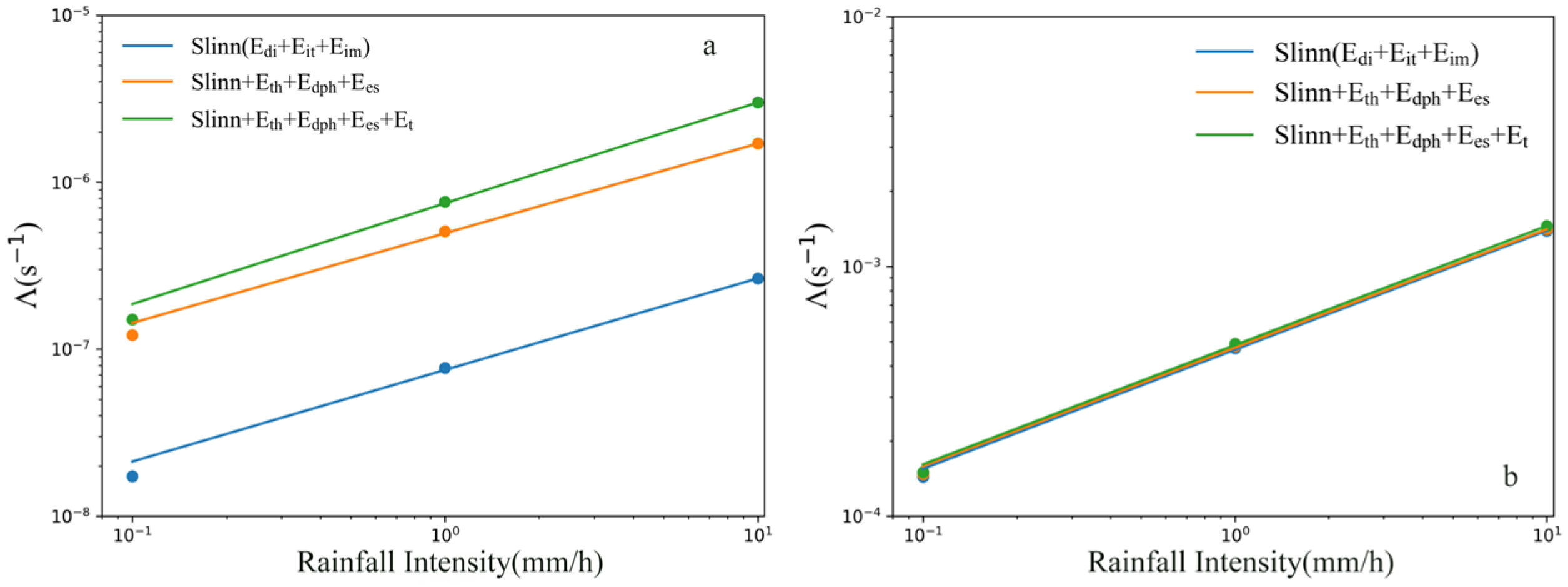
In the formula, A and B are parameters related to factors such as the raindrop size spectrum, aerosol size spectrum, and collision efficiency. Assuming that the raindrop size spectrum follows a log-normal distribution and the raindrop diameter ranges from 0.2 to 2 mm, the relationship between the scavenging coefficient of monodisperse aerosol particles with a diameter of 0.5 μm and the rainfall intensity is shown in Figure 2a. The introduction of the thermophoresis mechanism, diffusiophoresis mechanism, electrostatic interaction mechanism, and turbulent effect mechanism makes the scavenging coefficient about seven times higher than that when only using the three mechanisms proposed by Slinn, which is nearly one order of magnitude higher. Therefore, when parameterizing the scavenging coefficient of monodisperse aerosol particles, especially for particles within the accumulation mode range, the influence of the collision efficiency needs to be carefully considered.

When studying the scavenging coefficient of aerosols within the full-scale range, the average mass scavenging coefficient is usually used. The average mass scavenging coefficient is related to the raindrop size spectrum, the aerosol size spectrum, the terminal settling velocity of raindrops, and the collision efficiency. When the raindrop size spectrum, the aerosol size spectrum, and the raindrop settling velocity are given, the scavenging coefficient of polydisperse aerosols is only related to the collision efficiency. Assuming that both the raindrop size spectrum and the aerosol size spectrum are distributed in the form of a log-normal function, the particle size distribution range of aerosols is from 0.001 to 10 μm, and the raindrop diameter distribution range is from 0.2 to 2 mm. The relationship between the average mass scavenging coefficient and the rainfall intensity is shown in Figure 2b. The three lines almost overlap. It can be seen that, when considering rainfall scavenging within the full-scale range, the selection of the collision efficiency formula has little effect on the scavenging coefficient.

In conclusion, when studying the scavenging coefficient of monodisperse aerosols, especially for particles within the accumulation mode range, the collision efficiency formula should be carefully selected. However, when calculating the scavenging coefficient of aerosols within the full-scale range, the selection of the collision efficiency has little impact on the results. This is consistent with the research results of Peng Hong [25] and Yao Keya et al. [26].

2.3. The Influence of Raindrop Size Spectrum on the Scavenging Coefficient

The raindrop size spectrum refers to the number distribution of raindrops of different sizes in a unit volume. Clarifying the detailed information of the raindrop size spectrum is of great significance for the rainfall scavenging mechanism, estimating the scavenging coefficient, improving numerical weather models, and evaluating artificial rainfall enhancement [4,27]. Since Marshall and Palmer [28] found in 1948 that the raindrop size spectrum could be approximated as an exponential distribution, some scholars have conducted in-depth research on this and found that the raindrop size spectrum can not only be regarded as an exponential distribution but also conforms to the Gamma distribution [29] and the log-normal distribution [30]. Among them, the exponential distribution is also known as the M-P distribution [28]:

$$N\left(D_p\right)=N_0\exp \left(-\phi D_p\right)$$

(7)

In the formula, N₀ = 8000 m⁻³ mm⁻¹, φ = 4.1 · I^−0.21 mm⁻¹, and I is the rainfall intensity in mm/h. Studies have shown [31] that the M-P distribution is more suitable for stable stratiform cloud rainfall. For rainfall with large fluctuations in the cloud, it has large deviations in the range of small and large raindrops.

The Gamma distribution adds a new parameter based on the exponential distribution:

$$N\left(D_p\right)=N_0{D}_p^{\gamma }\exp \left(-\phi D_p\right)$$

(8)

In the formula, when γ = 0, the Gamma distribution becomes the M-P distribution. When γ > 0, the curve bends upward, and vice versa. Therefore, raindrop size spectra of different shapes can be fitted by adjusting the parameter γ. Compared with the M-P distribution, the Gamma distribution improves the fitting accuracy in the range of small and large raindrops and is more universal.

The log-normal distribution is more complex than the previous two distribution forms, and its expression is as follows:

$$N\left(D_p\right)={\displaystyle \frac{N}{D_p\sqrt{2\pi }\ln \sigma }}\exp \left[-{\displaystyle \frac{{\ln }^2\left(D_p/D_{dg}\right)}{2{\ln }^2\sigma }}\right]$$

(9)

In the formula, N is the initial total number concentration of raindrops, in m⁻³; D_dg is the average size of raindrops, in mm; σ is the geometric standard deviation of raindrops. Among them, these three parameters are all functions of the rainfall intensity, as shown in

Table 2. Relationship between rainfall intensity and log-normal distribution parameters.

Literature Source	N (m−3)	Ddg (mm)	σ
Feingold and Levin [30]	172 ∙ I0.22	0.72 ∙ I0.23	1.43–3.1 × 10−4 ∙ I
Cerro et al. [32]	194 ∙ I0.3	0.63 ∙ I0.23	(0.191–1.1 × 10−2lnI)0.5

.

It is assumed that light rain, moderate rain, and heavy rain are defined by rainfall intensities of 0.1, 1, and 10 mm/h, respectively, and the three types of raindrop size spectra are shown in Figure 3. The parameters used in the M-P exponential distribution are given by Marshall–Palmer [28], the parameters of the Gamma distribution are given by Wolf [33], and the log-normal distribution uses the parameters given by Feingold and Levin [30] as well as Cerro et al. [32].

As shown in Figure 3a,b, the raindrop size spectrum increases rapidly with the increase of the raindrop diameter and then decreases with the further increase of the raindrop diameter after reaching the peak value. Light rain reaches the peak value first, followed by moderate rain, and heavy rain reaches the peak value last. With the increase in rainfall intensity, the peak value shifts to the right and the peak width becomes larger, indicating that, with the increase in rainfall intensity, the width of the raindrop size spectrum increases and the distribution range of raindrop sizes becomes larger. As shown in Figure 3c,d, the raindrop size spectrum decreases with the increase of the raindrop diameter. This may be related to the influence of physical processes such as evaporation and fragmentation of raindrops during their fall. When the raindrop sizes are the same, the greater the rainfall intensity, and the greater the value of the raindrop size spectrum. This is because rainfall intensity indirectly indicates that precipitation is proportional to the raindrop diameter and the number concentration of raindrops. That is, when the rainfall intensity increases, if the raindrop diameters are the same, the number concentration of raindrops becomes larger.

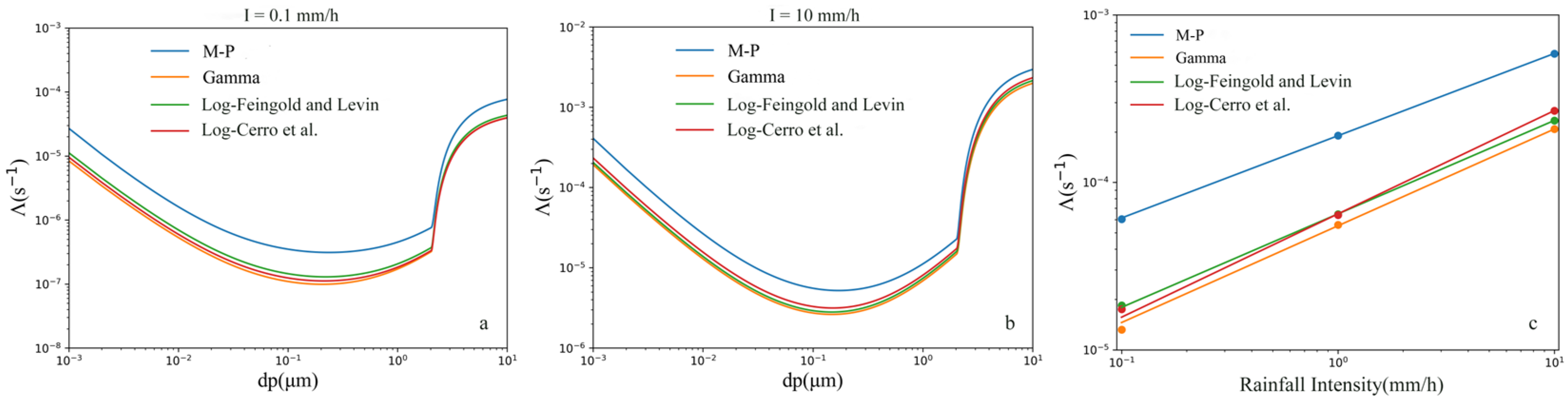
When the collision efficiency and the raindrop velocity are given, the value of the scavenging coefficient for monodisperse aerosol particles is only related to the raindrop size spectrum. The influence of three different types of raindrop size spectra under different rainfall intensities on the scavenging coefficient is shown in Figure 4. It is found that the scavenging coefficient obtained when the raindrop size spectrum follows the M-P distribution is larger than that obtained from other types of raindrop size spectra. For a rainfall intensity of I = 10 mm/h, the scavenging coefficient calculated according to the M-P distribution is about twice as large as that calculated according to the Gamma distribution. For I = 0.1 mm/h, the scavenging coefficient of the M-P distribution is about three times that of the Gamma distribution. This may be because the M-P distribution has a higher number concentration of raindrops and a higher proportion of small raindrops. Also, the collision efficiency of small raindrops with aerosols is higher than that of large raindrops, which leads to a higher scavenging coefficient obtained from the M-P distribution. With the increase of the rainfall intensity, the differences in the scavenging coefficients calculated from various types of raindrop size spectra also decrease. This is because, as the rainfall intensity increases, the raindrop sizes also approach those of large raindrops.

When the aerosol size spectrum distribution, collision efficiency, and raindrop velocity are given, the average mass scavenging coefficient of polydisperse aerosols is only related to the raindrop size spectrum distribution function. Assuming that the aerosol size spectrum is distributed in the form of a log-normal function, the particle size distribution range of aerosols is from 0.001 to 10 μm, and the raindrop diameter distribution range is from 0.2 to 2 mm. For the different types of raindrop size spectra above, the relationship between the average mass scavenging coefficient and the rainfall intensity is shown in Figure 4c. It can be seen that the scavenging coefficient calculated using the raindrop size spectrum of the M-P distribution is larger than that calculated using the raindrop size spectra of the Gamma distribution and the log-normal distribution, with a maximum difference of about 2.4 times. However, there is not much difference between the results of the Gamma distribution and the log-normal distribution.

A large number of studies have found [31,34,35,36] that the raindrop size spectra of rainfall in different cloud types, such as stratiform clouds, convective clouds, and mixed clouds, etc., vary greatly. Taking the study of Wang Fuzeng et al. [36] as an example, the results show that, when fitting the three different types of rainfall situations above, it is found that the fitting result of the Gamma distribution is better than that of the M-P distribution. The fitting results are shown in

Table 3. Droplet spectral distribution functions (including the M-P distribution and the Gamma distribution) for three different types of rainfall.

Types	M-P Distribution		Gamma Distribution
	N(Dp) m−3 mm−1	R2	N(Dp) m−3 mm−1	R2
Mixed cloud	N(Dp) = 221.29 ∙ exp(−1.689Dp)	0.8787	N(Dp) = 8.53 × 107 ∙ Dp8.876 ∙ exp(−15.02Dp)	0.9615
Convective cloud	N(Dp) = 82.74 ∙ exp(−0.8759 Dp)	0.9520	N(Dp) = 386.85 ∙ Dp1.331 ∙ exp(−2.283Dp)	0.9649
Stratiform cloud	N(Dp) = 452.92 ∙ exp(−3.052 Dp)	0.9194	N(Dp) = 1.19 × 1011 ∙ Dp 12.786 ∙ exp(−23.941 Dp)	0.9932

.

As shown in Table 3, for rainfall in different cloud types, the raindrop size spectrum distributions vary significantly. For example, in the M-P distribution, the initial concentration N₀ of the raindrop size spectrum of stratiform clouds is larger than that of mixed clouds and convective clouds. However, the slope factor φ is also larger than that of other cloud types. This will result in the number of small raindrops in stratiform clouds being higher than that in mixed clouds and convective clouds, while the number of large raindrops is lower than that in the other two cloud types.

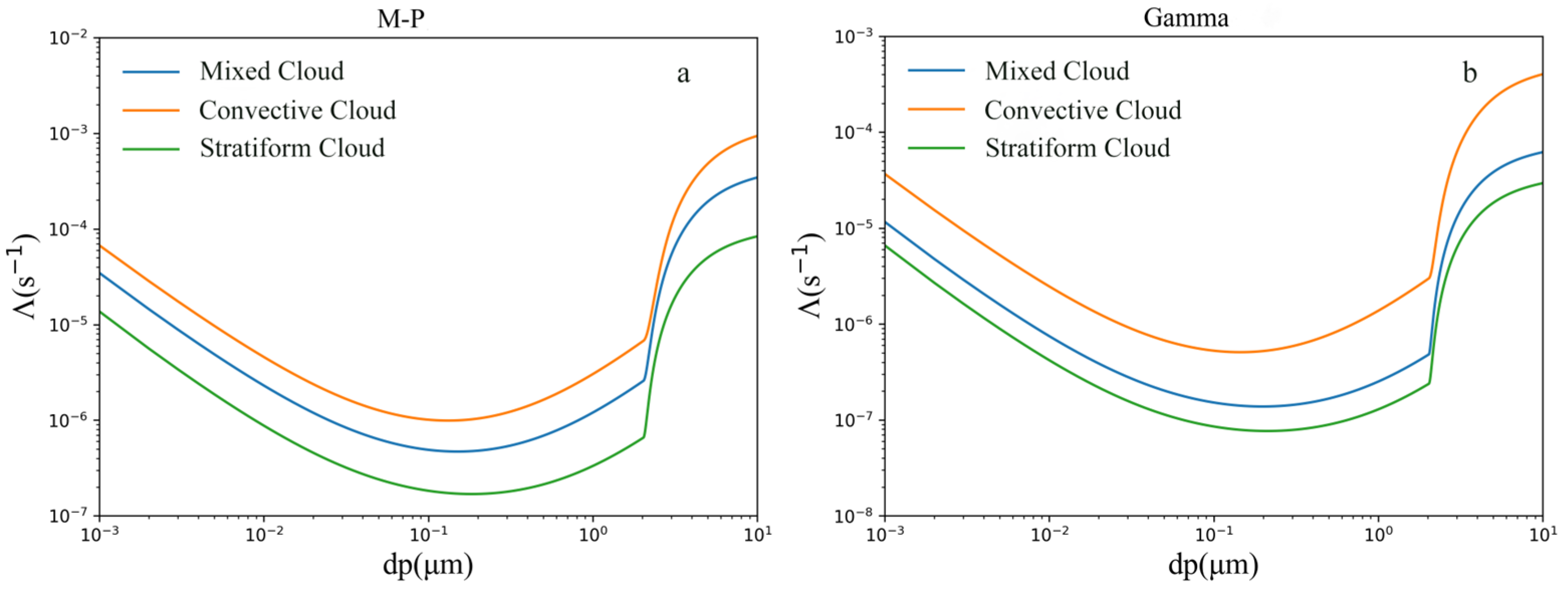
Figure 5 shows the influence of the raindrop size spectra (including the M-P distribution and the Gamma distribution) of rainfall in three different cloud types, namely, mixed clouds, convective clouds, and stratiform clouds, on the scavenging coefficient. It can be seen that the rainfall in different cloud types has a significant impact on the scavenging coefficient. Whether it is the M-P distribution or the Gamma distribution, the calculation results of rainfall in convective clouds are larger than those in mixed clouds and stratiform clouds. This is because the average diameter and the dominant diameter of raindrops in stratiform cloud precipitation are relatively small. The average diameters of raindrops in convective cloud precipitation and mixed cloud precipitation are basically the same, but the dominant diameter of raindrops in convective cloud precipitation is larger than that in mixed cloud precipitation [36]. The proportion of large particles in convective cloud precipitation is relatively large, and the contribution rate of precipitation is also large, which leads to a larger amount of convective cloud precipitation. Therefore, compared with other types, the scavenging coefficient of convective clouds is larger.

2.4. The Influence of Aerosol Spectrum on the Scavenging Coefficient

Atmospheric aerosol refers to a mixed system composed of the atmosphere and various solid- and liquid-phase particles in the atmosphere. In a narrow sense, it specifically refers to various solid-phase (dry) and liquid-phase (wet) particles [37]. Aerosol particles can affect climate change by scattering and absorbing short-wave solar radiation, and can also affect cloud precipitation and thus indirectly affect the climate [38]. Aerosol particles of different scales have significant differences in their optical, chemical compositional, and toxicological properties. Accurately describing the aerosol spectrum distribution is of great significance for research on the physical and chemical properties of aerosols. The scale of atmospheric aerosol particles can often span 5–6 orders of magnitude. Common functions used to describe the aerosol particle spectrum include the log-normal distribution, Gamma distribution, Junge distribution, etc. The log-normal distribution is a mathematical function with a physical basis. It can fit the distribution of the entire range of atmospheric aerosol scales and has good consistency in fitting the spectral distributions of number concentration, mass concentration, and surface area [38]. Its expression is as follows:

$$n(d_{\mathrm{p}})={\displaystyle \sum _{i=1}^n\frac{N_{\mathrm{i}}}{\sqrt{2\pi }{d}_{\mathrm{p}}\ln {\sigma }_{\mathrm{i}}}}\exp \left[-{\displaystyle \frac{{\left(\ln d_{\mathrm{p}}-\ln R_{\mathrm{i}}\right)}^2}{2{\left(\ln {\sigma }_{\mathrm{i}}\right)}^2}}\right]$$

(10)

In the formula, n is the peak number of the aerosol particle size spectrum; N_i represents the total number concentration of the i-th mode of aerosols, in cm⁻³; σ_i is the geometric standard deviation of the i-th mode; R_i is the geometric mean diameter of the i-th mode, in μm. A log-normal distribution function curve can fit a unimodal particle size spectrum (n = 1), and a multimodal particle size spectrum is composed of the superposition of log-normal distribution curves in multiple modes. The aerosol particle spectrum distributions of different modes have different characteristics, and the superimposed spectrum distribution can well reflect the state of the aerosol spectrum distribution. The selection of log-normal distribution simulation parameters for different regional types is from Jaenicke [39], and the log-normal distribution parameters for different seasons in the same region are given by Cao Wei et al. [38], as shown in

Table 4. Parameters of three types of aerosol distribution, and the spectral parameters of the three-mode aerosol in different seasons in Beijing. SP stands for spring; SU stands for summer; FA stands for autumn; WI stands for winter.

Type		I			II			III
		N1 (cm−3)	R1 (μm)	σ1	N2 (cm−3)	R2 (μm)	σ2	N3 (cm−3)	R3 (μm)	σ3
Ocean		133	0.008	4.53	66.6	0.266	1.62	3.1	0.58	2.48
Rural		6650	0.015	1.67	147	0.054	3.6	1990	0.084	1.84
City		99,300	0.013	1.75	1110	0.014	4.64	36,400	0.05	2.17
Beijing	SP	10,200	0.016	2	12,400	0.050	1.9	5700	0.126	1.9
	SU	6600	0.019	1.9	10,100	0.054	1.8	6900	0.148	1.8
	FA	5800	0.020	1.9	11,900	0.052	1.9	8500	0.146	1.8
	WI	6300	0.019	2	11,500	0.053	1.8	9400	0.117	1.9

.

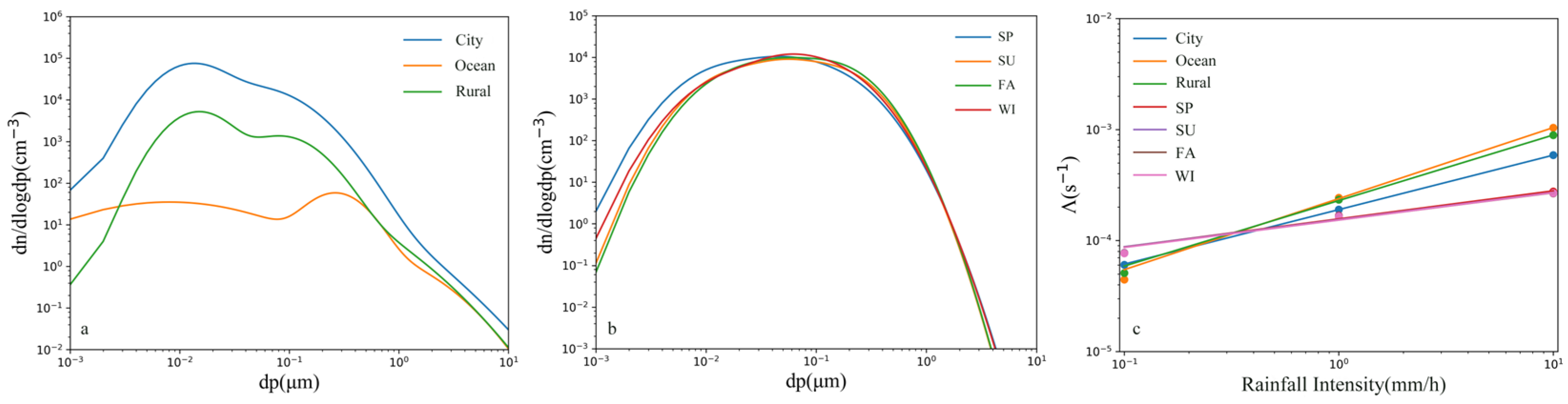
Figure 6 shows the aerosol spectrum distributions of different regional types and the aerosol spectrum distributions of different seasons in the same region. The aerosol spectrum distributions of different regional types vary significantly. Obviously, whether in urban, rural, or marine areas, the number concentration of the first mode is greater than that of the second and third modes. The geometric mean diameters of the three modes of urban aerosols are all within the Aitken mode range, so urban aerosols can be considered to be dominated by Aitken-mode particles. For rural aerosols, the second and third modes are both in the accumulation mode, but the number concentration is lower than that of the first mode. For marine aerosols, the first mode is in the Aitken mode, but the geometric standard deviation is relatively large, resulting in an expanded scale range of the aerosol spectrum distribution. For the aerosol spectrum distributions in different seasons in Beijing there is not much difference, but the number concentration is lower than that of urban aerosols.

When the raindrop size spectrum, raindrop settling velocity, and collision efficiency are given, the average mass scavenging coefficient of polydisperse aerosols is only related to the aerosol size spectrum. The particle size distribution range of aerosols is between 0.001 and 10 μm, and the raindrop size range is between 0.2 and 2 mm, as shown in Figure 6c. For urban aerosols, when the aerosol size spectrum follows the log-normal distribution, there is a significant difference between the parameters given by Jaenicke and the measured results in Beijing, with a maximum difference of about 1.5 times, mainly in the range of high rainfall intensities. It can be seen that the aerosol size spectrum has a great influence on the scavenging coefficient. This indicates that, even if the same type of aerosol size spectrum is used, when there is a large difference between the empirical parameters and the measured parameters, the difference in the results of the scavenging coefficient will also increase, as happened in the case of the parameters given by Jaenicke and the measured results in Beijing. Therefore, when studying the rainfall scavenging coefficient, it is best to use the locally measured aerosol size spectrum to reduce the influence brought about by the aerosol size spectrum distribution. However, for the same region, the influence of the aerosol size spectrum distribution function on the scavenging coefficient under different seasonal conditions can be ignored. Therefore, the seasonal average aerosol size spectrum can be used to represent the local aerosol size spectrum.

2.5. The Influence of Raindrop Terminal Velocity on the Scavenging Coefficient

In the rainfall scavenging coefficient formula, the raindrop terminal settling velocity V(D_p) is an important parameter, which refers to the velocity of raindrops in the atmosphere. Under the action of gravity and resistance, the velocity of raindrops will gradually increase until it reaches a stable velocity. The terminal velocity of raindrops is determined by the raindrop diameter, atmospheric density, and viscosity. Since different rainfall forms may lead to different falling patterns, researchers have carried out a large number of observations and laboratory simulations to obtain data on the raindrop falling process, and have proposed corresponding calculation formulas, which are listed in

Table 5. Calculation formula for terminal settling velocity V(D_p) of raindrops (m/s).

Num	Author	Formula	Source
1	Best, A.C.	V(Dp) = 9.85 {1 − exp[−(Dp/0.00177)1.147]}	[44]
2	Kessler, E.	V(Dp) = 130Dp0.5	[45]
3	Atlas, D.	V(Dp) = 9.65–10.3exp(−600Dp)	[42]
4	Atlas, D.	V(Dp) = 17.67(100Dp)0.67	[46]
5	Willis, P.T.	V(Dp) = 4854Dp exp(−195Dp)	[43]
6	Brandes, E.A.	V(Dp) = −0.1021 + 4932Dp − (0.9551Dp2 − 79.34Dp3 + 2362Dp4) × 106	[47]

, where the unit of D_p is m. In recent years, some scholars have studied the influence of turbulence on the terminal velocity of raindrops. Both in qualitative and quantitative studies, it has been found that the terminal falling velocity of raindrops decreases with the increase in turbulence intensity. Under turbulence of medium and low intensity, the actual measured values are closer to the terminal settling velocity of raindrops measured in the laboratory [40,41]. In the study by Zheng et al. [41], under the condition of medium and low turbulence intensity with a turbulence dissipation rate of ε < ε_60%, the actually measured average falling velocity of raindrops is close to the velocity measured by Atlas et al. [42] in the laboratory. However, under high-intensity turbulence, that is, ε > ε_80%, the actually measured values are slightly lower, but the standard deviation also increases accordingly. Therefore, considering the actual situation, we will use laboratory measurements instead of field measurements under turbulent conditions. The experimental data of Kinzer et al. have been fitted [43], and the result is basically consistent with the velocity curve fitted by Atlas et al., as shown in Figure 7a. In the subsequent content of this article, the Willis velocity formula will be used to calculate the raindrop terminal settling velocity.

The relationship between the raindrop terminal settling velocity distribution and the raindrop diameter is shown in Figure 7a. Except for the velocity curves of Atlas (1977) [46] and Kessler [45], the velocity distributions of the others are basically the same, within the raindrop diameter range of 0–5 mm. When the raindrop size spectrum, the aerosol size spectrum, and the collision efficiency formula are given, the scavenging coefficient is related to the raindrop terminal settling velocity. As shown in Figure 7b, it is found that the results calculated by the velocity formulas of Atlas (1977) [46] and Kessler [45] are relatively large, and the results calculated by other velocity formulas are similar. The scavenging coefficients calculated by the velocity formulas of Kessler [45] and Atlas (1973) [42] have a maximum difference of about 1.7 times, and the differences are mainly concentrated in the range of low rainfall intensities.

3. Basic Estimation and Analysis of the Rainfall Scavenging Prediction Model

For the urban atmosphere, rainfall is the most fundamental natural scavenging pathway for particulate pollutants, and wet scavenging can improve the near-surface air environment in a short period. Over the past decade or so, many achievements have been made in the research on the spatiotemporal variation patterns, sources, formation, and chemical compositions of aerosols such as PM₁₀, PM_2.5, and PM₁ [48,49]. However, current research has not deeply discussed and analyzed the scavenging situation of small-sized particles during the rainfall process and the estimation of their scavenging effects. Therefore, this paper selects the measured data of Guangzhou City, Tianjin City, and Hefei City, and establishes a theoretical model for the rainfall scavenging of polydisperse aerosols, which is used to predict the scavenging coefficient of aerosols by rainfall, estimate the changing trend of the aerosol mass concentration with different rainfall times, and conduct verification and modification in combination with actual rainfall events.

3.1. Selection of Raindrop Size Spectrum and Aerosol Spectrum

Qiu et al. [50] conducted a study on the rainfall data in the Guangzhou area and found that there were significant differences in the raindrop size spectra fitted for different rainfall types. Therefore, they classified the raindrop size spectra of different types of rainfall, and the specific results of the raindrop size spectrum parameters are shown in

Table 6. Parameters of raindrop spectra for different rainfall types.

Type	N0 (m−3∙mm−1)	χ	ψ
Downpour (I > 25 mm/h)	6183.9	5.0	−0.26
Heavy rain (5 < I < 25 mm/h)	9446.5	4.8	−0.21
Light rain (I < 5 mm/h)	11,873.5	4.0	−0.18

.

Another distribution mode of the raindrop size spectrum, the Gamma distribution, adds a new parameter on the basis of the exponential distribution. By adjusting the newly added parameter, raindrop size spectra of different shapes can be fitted. Compared with the M-P distribution, the Gamma distribution improves the fitting accuracy in the range of small and large raindrops and is more universal. The expression is as follows:

$$N\left(D_p\right)=N_0{D}_p^{\gamma }\exp \left(-\phi D_p\right)$$

(11)

In the formula, γ is the shape factor. When γ > 0, the curve bends upward; when γ < 0, the curve bends downward; when γ = 0, the Gamma distribution becomes the M-P distribution. The raindrop size spectrum in Hefei City adopts the Gamma distribution given by Jin et al. [51]. Similarly, the parameters of different types of rainfall are classified and processed, and the specific parameters are shown in

Table 7. Gamma distribution parameters for different rainfall types.

Type	N0 (m−3∙mm−1)	γ	χ	ψ
Stratiform cloud (0 < I < 5 mm/h)	2.51 × 107	9.1	11.4	−0.1
Convective cloud (I > 5 mm/h)	3.16 × 105	5.6	8.648	−0.15

.

The raindrop size spectrum of the Gamma distribution can be normalized [43,52,53,54]. Compared with the standard Gamma raindrop spectrum, the normalized Gamma distribution has better flexibility and can simultaneously characterize the spectral shapes of raindrops ranging from small to large [54]. The raindrop size spectrum in Tianjin City adopts the Gamma distribution given by Han Yi [55], and the expression is as follows:

$$N(D_p)=N_{w}f(\gamma ){\left(D_p/D_m\right)}^{\gamma }\exp \left[-\left(4+\gamma \right)\left(D_p/D_m\right)\right]$$

(12)

$$f(\gamma )={\displaystyle \frac{6}{4^4}}{\displaystyle \frac{{\left(4+\gamma \right)}^{\gamma +4}}{\Gamma \left(\gamma +4\right)}}$$

(13)

In the formula, N_w is the generalized intercept parameter, in mm⁻¹∙m⁻³; D_m is the mass-weighted mean diameter, in mm; Γ is the Gamma function. The specific parameters are shown in

Table 8. Normalized Gamma distribution parameters.

Type	Nw (mm−1∙m−3)	Dm (mm)	γ
Stratiform cloud (0 < I < 5 mm/h)	6903 ∙ I0.57	1.0 ∙ I0.08	3.7
Convective cloud (I > 5 mm/h)	8771 ∙ I0.32	0.97 ∙ I0.13	2.086

.

The aerosol size spectrum distribution describes the number distribution of aerosol particles at different scales, specifically manifested as the particle number or mass distribution in each particle size segment. The log-normal distribution is a mathematical function with a physical basis, which can fit the distribution of the entire range of atmospheric aerosol scales, and has good consistency in fitting the spectral distributions of number concentration, mass concentration, and surface area [38]:

$$n(d_{\mathrm{p}})={\displaystyle \sum _{i=1}^n\frac{N_{\mathrm{i}}}{\sqrt{2\pi }{d}_{\mathrm{p}}\ln {\sigma }_{\mathrm{i}}}}\exp \left[-{\displaystyle \frac{{\left(\ln d_{\mathrm{p}}-\ln R_{\mathrm{i}}\right)}^2}{2{\left(\ln {\sigma }_{\mathrm{i}}\right)}^2}}\right]$$

(14)

In the formula, n is the number of peaks in the aerosol particle size spectrum; N_i represents the total number concentration of the i-th mode of aerosols, in units of cm⁻³; σ_i is the geometric standard deviation of the i-th mode; R_i is the geometric mean diameter of the i-th mode, in units of μm.

Han Bingxue [56] carried out a bimodal fitting of the aerosol size spectrum in Guangzhou City under different seasonal conditions, as shown in

Table 9. Bimodal distribution of aerosol scale spectra for different seasons.

Season	Mode 1			Mode 2
	N1 (cm−3)	σ1	R1 (μm)	N2 (cm−3)	σ2	R2 (μm)
Spring	11,864	2.02	0.056	3873	1.77	0.144
Summer	10,599	1.89	0.051	1269	1.56	0.177
Fall	5817	2.03	0.021	6373	1.82	0.127
Average	9426.7	1.98	0.0526	3838.3	1.72	0.1493

. According to the research content in Section 2, the influence of the aerosol size spectrum in different seasons on the scavenging coefficient is not significant. Therefore, in this chapter, the seasonal average value of the aerosol size spectrum in Guangzhou City is used.

Huang Honglian et al. [57] conducted a study on the aerosol size spectrum in Hefei City and found that the aerosol size spectrum in the Hefei area shows a unimodal distribution. The specific parameters are shown in

Table 10. Unimodal distribution of aerosol scale spectra in Hefei City.

	N1 (cm−3)	σ1	R1 (μm)
Number concentration spectrum	240.56	1.2	0.36

.

Liang Si et al. [58] carried out a trimodal fitting of the aerosol size spectrum in Tianjin City, and the specific parameters are shown in

Table 11. Tianjin aerosol scale spectra three-mode distribution.

Mode	Ni (cm−3)	σi	Ri (μm)
Mode1	9.92 × 103	2.11	0.0396
Mode2	6.82 × 103	1.67	0.1334
Mode3	4.59 × 103	1.31	0.3892

.

3.2. Validation and Modification of the Model for Rainfall Scavenging of Polydisperse Aerosols

The measured rainfall data are sourced from 1 January 2021 to 31 December 2023. In order to obtain accurate data results, it is necessary to count only the valid data and ensure the continuity of the data. Therefore, during the observation period, only the rainfall events with continuous rainfall exceeding 5 h are selected, the abnormal values are removed, and statistical analysis is carried out on them.

The variation of the PM_2.5 concentration with the rainfall time during continuous rainfall is shown in Figure 8. The abscissa in the figure represents the rainfall duration (in hours), and the ordinate represents the PM_2.5 concentration (in μg/m³) measured in the corresponding hour. Figure 8a,b, Figure 8c,d and Figure 8e,f are randomly selected from the measured data of Guangzhou City, Hefei City, and Tianjin City, respectively.

It can be seen in Figure 8 that the PM_2.5 concentration shows an obvious downward trend with the increase in rainfall time. For the actual rainfall process, according to Equation (3), the scavenging coefficient is calculated. It can be seen that the actual rainfall scavenging coefficients of rainfall for PM_2.5 in Guangzhou City in Figure 8 are 2.19 × 10⁻⁵ s⁻¹ and 2.82 × 10⁻⁵ s⁻¹. The measured rainfall scavenging coefficients in Hefei City are 1.57 × 10⁻⁵ s⁻¹ and 2.54 × 10⁻⁵ s⁻¹, respectively, and the measured rainfall scavenging coefficients in Tianjin City are 1.304 × 10⁻⁵ s⁻¹ and 3.92 × 10⁻⁵ s⁻¹, respectively.

According to the previously established prediction model for the rainfall scavenging of polydisperse aerosols, the variation characteristics of PM_2.5 over time estimated by the prediction model for the rainfall scavenging of polydisperse aerosols can be obtained. As shown in Figure 9, compared with the measured values, the trend of the theoretical prediction model is basically consistent with that of the measured values. This proves that the established model can accurately predict the variation trend of the atmospheric pollutant PM_2.5 over time to a certain extent.

It should be noted that the parameters in the above theoretical prediction model, such as the raindrop size spectrum and the aerosol size spectrum, are all from local measurements, and the collision efficiency is obtained by superimposing the results of Brownian diffusion, interception effect, inertial collision, thermophoresis, diffusiophoresis, electrostatic effect, and turbulent effect. As described in Section 2.2, within the full-scale range, the variation of the scavenging coefficient of polydisperse aerosols by rainfall has little relation to the selection of the collision efficiency formula. However, in the process of simulating the variation of the scavenged concentration of PM_2.5 by rainfall over time, it is found that, even though the variation of the scavenging coefficient of polydisperse aerosols by rainfall has little relation to the selection of the collision efficiency formula, the differences between the collision efficiency formulas will gradually magnify as time goes by, as shown in Figure 10.

As shown in Figure 10, the differences among the theoretical scavenging coefficients of Slinn’s three-mechanism approach, the six-mechanism approach, and the approach using the six mechanism plus the turbulent effect gradually expand over time, with a maximum difference of about one time. It can be seen that, even if the values of the scavenging coefficients do not differ greatly, the differences will gradually increase as time goes on. In addition, when the turbulent effect is introduced, the theoretical prediction is closer to the measured value, which indicates that the influence of the turbulent effect on the scavenging of aerosols cannot be ignored.

In addition, we calculated the measured statistical data and compared them with the calculated values of the theoretical prediction model and found that there is a linear relationship between them. Specifically, this is shown in Figure 11.

In Figure 11, it can be seen that there is a linear relationship between the calculated values obtained by the rainfall scavenging coefficient model and the actual measured values. Through least squares fitting, its specific mathematical expression is as follows:

Λ_s = 0.498 × 10⁻⁵ + 1.025Λ_m R² = 0.828

(15)

Λ_s = 1.035Λ_m − 0.036 × 10⁻⁵ R² = 0.823

(16)

Λ_s = 0.903Λ_m − 1.11 × 10⁻⁵ R² = 0.813

(17)

Therefore, for the calculated values of the scavenging coefficient model of particles in the PM_2.5 range, under the rainfall conditions in Guangzhou City, Hefei City, and Tianjin City, Equations (15)–(17) can be used for correction, respectively.

4. Conclusions

This study undertakes a comprehensive and in-depth exploration of the rainfall scavenging coefficient of aerosols, culminating in several significant and well-founded conclusions. In the context of scavenging coefficient calculations, the selection of the collision efficiency formula proves to be a critical determinant, particularly for monodisperse aerosols, with a pronounced impact observed among particles within the accumulation mode size spectrum. In contrast, its influence on the computation of scavenging coefficients for aerosols spanning the entire particle size continuum is comparatively less substantial.

The distribution characteristics of the raindrop size spectrum exert a profound and demonstrable effect on the calculated values of the scavenging coefficient. Specifically, scavenging coefficients derived from the Marshall–Palmer (M-P) raindrop size distribution exhibit a significant elevation compared to those obtained from alternative distributions, with the maximum differential reaching up to 2.4-fold. Conversely, the results yielded by the Gamma and logarithmic distributions display a relatively marginal disparity. This underscores the imperative of taking into account the locale-specific raindrop size spectrum characteristics in aerosol scavenging research. Moreover, the precision of aerosol particle size spectrum parameters is of paramount importance; substantial discrepancies between empirical and measured parameters can lead to considerable deviations in scavenging coefficient estimations. However, it is noteworthy that the seasonal fluctuations in aerosol scavenging coefficients within a given region are minimal, thereby justifying the utilization of seasonal mean values as a representative metric for local aerosol particle size spectra. With respect to the selection of raindrop terminal velocity formulas, under conditions of moderate to low turbulence intensities, laboratory-calibrated velocity formulations are deemed appropriate for computational purposes.

A predictive model for the rainfall scavenging of polydisperse aerosols was developed and subsequently validated through case-study analyses of Guangzhou, Hefei, and Tianjin. The model-estimated temporal dynamics of PM_2.5 concentrations exhibit a high degree of congruence with the trends observed in measured data. This study further reveals that, although the initial impact of different collision efficiency assumptions on scavenging coefficients is negligible, these disparities gradually become more pronounced over time. The incorporation of turbulent effects significantly enhances the concordance between theoretical predictions and measured values, thereby emphasizing the non-negligible role of turbulence in the aerosol scavenging mechanism. Additionally, a robust linear relationship has been established between the theoretical calculations of the rainfall scavenging coefficient model and the corresponding field-measured values, as encapsulated in the equations Λ_s = 0.498 × 10⁻⁵ + 1.025Λ_m, Λ_s = 1.035Λ_m − 0.036 × 10⁻⁵, and Λ_s = 0.903Λ_m − 1.11 × 10⁻⁵.

References

1. Textor, C.; Schulz, M.; Guibert, S.; Kinne, S.; Balkanski, Y.; Bauer, S.; Berntsen, T.; Berglen, T.; Boucher, O.; Chin, M. Analysis and quantification of the diversities of aerosol life cycles within AeroCom. Atmos. Chem. Phys. 2006, 6, 1777–1813. [Google Scholar] [CrossRef]
2. Radke, L.F.; Hobbs, P.V.; Eltgroth, M.W. Scavenging of aerosol particles by precipitation. J. Appl. Meteorol. Climatol. 1980, 19, 715–722. [Google Scholar] [CrossRef]
3. Sportisse, B. A review of parameterizations for modelling dry deposition and scavenging of radionuclides. Atmos. Environ. 2007, 41, 2683–2698. [Google Scholar] [CrossRef]
4. Wang, X.; Zhang, L.; Moran, M.D. Uncertainty assessment of current size-resolved parameterizations for below-cloud particle scavenging by rain. Atmos. Chem. Phys. 2010, 10, 5685–5705. [Google Scholar] [CrossRef]
5. Wang, X.; Zhang, L.; Moran, M.D. On the discrepancies between theoretical and measured below-cloud particle scavenging coefficients for rain–a numerical investigation using a detailed one-dimensional cloud microphysics model. Atmos. Chem. Phys. 2011, 11, 11859–11866. [Google Scholar] [CrossRef]
6. Gong, W.; Stroud, C.; Zhang, L. Cloud processing of gases and aerosols in air quality modeling. Atmosphere 2011, 2, 567–616. [Google Scholar] [CrossRef]
7. Wang, X.; Zhang, L.; Moran, M.D. Development of a new semi-empirical parameterization for below-cloud scavenging of size-resolved aerosol particles by both rain and snow. Geosci. Model Dev. 2014, 7, 799–819. [Google Scholar] [CrossRef]
8. Slinn, W. Precipitation Scavenging, in Atmospheric Sciences and Power Production–1979; Division of Biomedical Environmental Research, US Department of Energy: Washington, DC, USA, 1983; pp. 466–532. [Google Scholar]
9. Chate, D.M.; Murugavel, P.; Ali, K.; Tiwari, S.; Beig, G. Below-cloud rain scavenging of atmospheric aerosols for aerosol deposition models. Atmos. Res. 2011, 99, 528–536. [Google Scholar] [CrossRef]
10. Chen, M.; Feng, Q.; Zuo, Y.; Gao, X.; Huang, J.; Wang, H. A Parameterized Study on Rainfall Removal of Aerosols. Aerosol Sci. Eng. 2023, 7, 355–367. [Google Scholar] [CrossRef]
11. Langmuir, I. The production of rain by a chain reaction in cumulus clouds at temperatures above freezing. J. Atmos. Sci. 1948, 5, 175–192. [Google Scholar] [CrossRef]
12. Greenfield, S.M. Rain scavenging of radioactive particulate matter from the atmosphere. J. Atmos. Sci. 1957, 14, 115–125. [Google Scholar] [CrossRef]
13. Wang, P.K.; Pruppacher, H.R. An experimental determination of the efficiency with which aerosol particles are collected by water drops in subsaturated air. J. Atmos. Sci. 1977, 34, 1664–1669. [Google Scholar] [CrossRef]
14. Pinsky, M.; Khain, A.; Shapiro, M. Collision efficiency of drops in a wide range of Reynolds numbers: Effects of pressure on spectrum evolution. J. Atmos. Sci. 2001, 58, 742–764. [Google Scholar] [CrossRef]
15. Berthet, S.; Leriche, M.; Pinty, J.-P.; Cuesta, J.; Pigeon, G. Scavenging of aerosol particles by rain in a cloud resolving model. Atmos. Res. 2010, 96, 325–336. [Google Scholar] [CrossRef]
16. Hua, F.J.; Kang, Y.M.; Zhong, K. Influence of turbulent effect on the collection process of aerosols by raindrops. China Environ. Sci. 2017, 37, 13–20. [Google Scholar]
17. Gao, X.; Zuo, Y.; Wang, H. Influence of the Turbulence Effect on the Rainfall Scavenging Coefficient. Aerosol Sci. Eng. 2024, 8, 454–467. [Google Scholar] [CrossRef]
18. Slinn, W.G.N. Some approximations for the wet and dry removal of particlesand gases from the atmosphere. Water Air Soil Pollut. 1977, 7, 513–543. [Google Scholar] [CrossRef]
19. Laakso, L.; Grönholm, T.; Rannik, Ü.; Kosmale, M.; Fiedler, V.; Vehkamäki, H.; Kulmala, M. Ultrafine particle scavenging coefficients calculated from 6 years field measurements. Atmos. Environ. 2003, 37, 3605–3613. [Google Scholar] [CrossRef]
20. Chate, D.; Pranesha, T. Field measurements of sub-micron aerosol concentration during cold season in India. Curr. Sci. 2004, 86, 1610–1613. [Google Scholar]
21. Tost, H.; Jöckel, P.; Kerkweg, A.; Sander, R.; Lelieveld, J. A new comprehensive scavenging submodel for global atmospheric chemistry modelling. Atmos. Chem. Phys. 2006, 6, 565–574. [Google Scholar] [CrossRef]
22. Bae, S.Y.; Jung, C.H.; Kim, Y.P. Development and evaluation of an expression for polydisperse particle scavenging coefficient for the below-cloud scavenging as a function of rain intensity using the moment method. J. Aerosol Sci. 2006, 37, 1507–1519. [Google Scholar] [CrossRef]
23. Tinsley, B.; Rohrbaugh, R.; Hei, M.; Beard, K. Effects of image charges on the scavenging of aerosol particles by cloud droplets and on droplet charging and possible ice nucleation processes. J. Atmos. Sci. 2000, 57, 2118–2134. [Google Scholar] [CrossRef]
24. Scott, B. Theoretical estimates of the scavenging coefficient for soluble aerosol particles as a function of precipitation type, rate and altitude. Atmos. Environ. 1982, 16, 1753–1762. [Google Scholar] [CrossRef]
25. Peng, H.; Yu, Q. The Parameterization of the Precipitation on the washout of Aerosol Particles. Chin. J. Atmos. Sci. 1992, 16, 622–630. [Google Scholar]
26. Yao, K.; Guo, J.; Fu, Y.; Yong, L. Rain Scavenging of Aerosol Particles. Clim. Environ. Res. 1999, 4, 297–302. [Google Scholar]
27. Wang, Y.; Zhu, B.; Kang, H.; Jinhui, G. Theoretical and observational study on below-cloud rain scavenging of aerosol particles. J. Univ. Chin. Acad. Sci. 2014, 31, 306–313. [Google Scholar]
28. Marshall, J.S.; Palmer, W.M. The distribution of raindrops with size. J. Meteorol. 1948, 5, 165–166. [Google Scholar] [CrossRef]
29. Ulbrich, C.W. Natural variations in the analytical form of the raindrop size distribution. J. Clim. Appl. Meteorol. 1983, 22, 1764–1775. [Google Scholar] [CrossRef]
30. Feingold, G.; Levin, Z. The lognormal fit to raindrop spectra from frontal convective clouds in Israel. J. Clim. Appl. Meteorol. 1986, 25, 1346–1363. [Google Scholar] [CrossRef]
31. Chen, B.J.; Li, Z.H.; Liu, J.C. Model of raindrop size distribution in three types of precipitation. Acta Meteorol. Sin. 1998, 56, 123–129. [Google Scholar]
32. Cerro, C.; Codina, B.; Bech, J.; Lorente, J. Modeling raindrop size distribution and Z (R) relations in the western Mediterranean area. J. Appl. Meteorol. Climatol. 1997, 36, 1470–1479. [Google Scholar] [CrossRef]
33. Wolf, D.A.d. On the Laws-Parsons distribution of raindrop sizes. Radio Sci. 2001, 36, 639–642. [Google Scholar] [CrossRef]
34. Liu, C.Z.; Zhou, J.J.; Gu, J.; Huang, L. Characteristics of Raindrop Size Distribution in Chengdu. J. Appl. Meteorol. Sci. 2015, 26, 112–121. [Google Scholar]
35. Xu, W.; Su, D.; Hui, W. Characteristics of raindrop size spectrum in a heavy-precipitation process in Beijing. J. Atmos. Environ. Opt. 2017, 12, 8–14. [Google Scholar]
36. Wang, F.; Wang, Q.; He, S.; Xiaoping, G. Analysis of the characteristics of raindrop size spectrum in summer in Zheng’an, Guizhou. J. Chengdu Univ. Inf. Technol. 2020, 35, 689–696. [Google Scholar]
37. Coakley, J.A., Jr.; Cess, R.D.; Yurevich, F.B. The effect of tropospheric aerosols on the Earth’s radiation budget: A parameterization for climate models. J. Atmos. Sci. 1983, 40, 116–138. [Google Scholar] [CrossRef]
38. Cao, W.; Qiu, Y.J.; Shu, Z.Z.; Yong, L. Progress in atmospheric aerosol size distribution in China. Environ. Sci. Technol. 2017, 40, 87–96. [Google Scholar]
39. Jaenicke, R. Tropospheric Aerosols in Aerosol-Cloud-Climate Interactions; Hobbs, P.V., Ed.; Academic Press: Cambridge, MA, USA, 1993. [Google Scholar]
40. Thurai, M.; Bringi, V.; Gatlin, P.; Wingo, M. Raindrop fall velocity in turbulent flow: An observational study. Adv. Sci. Res. 2021, 18, 33–39. [Google Scholar] [CrossRef]
41. Zheng, H.; Zhang, Y.; Li, H.; Wu, Z.; Xie, Y.; Zhang, L. Raindrop Deformation in Turbulence. Geophys. Res. Lett. 2024, 51, e2024GL108627. [Google Scholar] [CrossRef]
42. Atlas, D.; Srivastava, R.; Sekhon, R.S. Doppler radar characteristics of precipitation at vertical incidence. Rev. Geophys. 1973, 11, 1–35. [Google Scholar] [CrossRef]
43. Willis, P.T. Functional fits to some observed drop size distributions and parameterization of rain. J. Atmos. Sci. 1984, 41, 1648–1661. [Google Scholar] [CrossRef]
44. Best, A.C. Empirical formulae for the terminal velocity of water drops falling through the atmosphere. Q. J. R. Meteorol. Soc. 1950, 76, 302–311. [Google Scholar] [CrossRef]
45. Kessler, E. On the distribution and continuity of water substance in atmospheric circulations. In On the Distribution and Continuity of Water Substance in Atmospheric Circulations; Springer: Berlin/Heidelberg, Germany, 1969; pp. 1–84. [Google Scholar]
46. Atlas, D.; Ulbrich, C.W. Path-and area-integrated rainfall measurement by microwave attenuation in the 1–3 cm band. J. Appl. Meteorol. Climatol. 1977, 16, 1322–1331. [Google Scholar] [CrossRef]
47. Brandes, E.A.; Zhang, G.; Vivekanandan, J. Experiments in rainfall estimation with a polarimetric radar in a subtropical environment. J. Appl. Meteorol. Climatol. 2002, 41, 674–685. [Google Scholar] [CrossRef]
48. Zhang, F.; Xu, L.; Chen, J.; Yu, Y.; Niu, Z.; Yin, L. Chemical compositions and extinction coefficients of PM2.5 in peri-urban of Xiamen, China, during June 2009–May 2010. Atmos. Res. 2012, 106, 150–158. [Google Scholar] [CrossRef]
49. Lin, Y.; Zou, J.; Yang, W.; Li, C.-Q. A Review of Recent Advances in Research on PM2.5 in China. Int. J. Environ. Res. Public Health 2018, 15, 438. [Google Scholar] [CrossRef] [PubMed]
50. Qiu, S.B.; Chen, J.H. The Distributions of Raindrop Sizes in Guangzhou. Chin. J. Radio Sci. 1995, 10, 73–77. [Google Scholar]
51. Jin, Q.; Yuan, Y.; Liu, H.; Shi, C.; Li, J. Analysis of microphysical characteristics of the raindrop spectrum over the area between the Yangtze River and the Huaihe River during summer. Acta Meteorol. Sin. 2015, 73, 778–788. [Google Scholar]
52. Torres, D.S.; Porrà, J.M.; Creutin, J.-D. A general formulation for raindrop size distribution. J. Appl. Meteorol. Climatol. 1994, 33, 1494–1502. [Google Scholar] [CrossRef]
53. Lee, G.W.; Zawadzki, I.; Szyrmer, W.; Sempere-Torres, D.; Uijlenhoet, R. A general approach to double-moment normalization of drop size distributions. J. Appl. Meteorol. 2004, 43, 264–281. [Google Scholar] [CrossRef]
54. Thurai, M.; Bringi, V. Application of the generalized gamma model to represent the full rain drop size distribution spectra. J. Appl. Meteorol. Climatol. 2018, 57, 1197–1210. [Google Scholar] [CrossRef]
55. Yi, H. Investigation of Raindrop Size Distribution and Its Potential Influential Factors During Warm Season over China. Master’s Thesis, Chinese Academy of Meteorological Sciences, Beijing, China, 2022. [Google Scholar]
56. Han, B.X. The Characteristics of Number Concentration and Size Distribution of Aerosols in the Urban Area of Guangzhou. Master’s Thesis, University of Chinese Academy of Sciences, Beijing, China, 2015. [Google Scholar]
57. Huang, H.; Huang, Y.; Rao, R. Observation and Research on the Characteristics of Aerosol Number Concentration and Size Distribution in Hefei Area. Infrared Laser Eng. 2006, S3, 390–395. [Google Scholar]
58. Liang, S.; Ma, N.; Xu, W.; Deng, B. Observation and research on the characteristics of aerosol size-distribution spectra in summer in the suburbs of Tianjin. Acta Sci. Nat. Univ. Pekin. 2012, 48, 246–252. [Google Scholar]
Figure 1. (a) The relationship between the collision efficiency and the particle size of the aerosol. The continuous curve represents the sum of the contributions from various physical mechanisms. The blue curve represents the situation where only the three mechanisms proposed by Slinn [8] are considered. The orange curve represents the combination of the three Slinn mechanisms plus the thermophoresis, diffusiophoresis, and electrostatic mechanisms. The green curve represents the combination of the three Slinn mechanisms, thermophoresis, diffusiophoresis, electrostatic mechanisms, and the turbulent effect. The dashed lines in different colors represent the contributions of different physical mechanisms to the collision efficiency. The meanings of the corresponding symbols are shown in Table 1. (b) The relationship between the scavenging coefficient and the particle size of the aerosol. The solid lines in different colors are similar to those in (a).
Atmosphere 16 00634 g001
Figure 2. Relationship between the scavenging coefficient of 0.5 μm particles and rainfall intensity (a), as well as relationship between average mass scavenging coefficient and rainfall intensity (b).
Atmosphere 16 00634 g002
Figure 3. Spectral distribution of raindrops under different rainfall intensities [28,30,32,33].
Atmosphere 16 00634 g003
Figure 4. The relationships between the scavenging coefficient and the particle size (a,b), as well as the relationship between the scavenging coefficient and the rainfall intensity under different conditions of raindrop spectra (c) [28,30,32,33].
Atmosphere 16 00634 g004
Figure 5. The relationship between scavenging coefficients and particle sizes for different rainfall types under the M-P distribution (a), as well as the relationship between scavenging coefficients and particle sizes for different rainfall types under the Gamma distribution (b) [36].
Atmosphere 16 00634 g005
Figure 6. (a) Aerosol spectra distributions in different regions [39]. (b) Aerosol spectral distributions in Beijing under different seasons [38]. (c) The relationship between the scavenging coefficient and rainfall intensity under different aerosol spectral distributions.
Atmosphere 16 00634 g006
Figure 7. The relationship between the terminal velocity of raindrops and the raindrop size (a), as well as the relationship between the scavenging coefficient and the rainfall intensity under different expressions (b) [42,43,44,45,46,47].
Atmosphere 16 00634 g007
Figure 8. Characteristics of hourly variation of PM2.5 concentration with rainfall in Guangzhou (a,b), Hefei (c,d), Tianjin (e,f).
Atmosphere 16 00634 g008
Figure 9. Measurement and simulation of the temporal variation characteristics of PM2.5.
Atmosphere 16 00634 g009
Figure 10. Characteristics of PM2.5 over time under different collision efficiencies.
Atmosphere 16 00634 g010
Figure 11. The relationships between the theoretical removal coefficients and the measured removal coefficients in Guangzhou City, Hefei City, and Tianjin City.
Atmosphere 16 00634 g011