A Novel Flood Probability Index Based on Radar Rainfall and Soil Moisture Estimates for a Small Vegetated Watershed in Southeast Brazil

Abstract

Floods result from intense and/or prolonged rainfall that exceeds the soil’s infiltration capacity, generating surface runoff and increasing river discharge. These events can cause substantial societal damage and may even lead to fatalities. In this study, we analyzed flood events in Lençóis Paulista, southeastern Brazil, between 2016 and 2024, by evaluating estimated precipitation and soil moisture conditions to develop a flood prediction index for the city. Precipitation estimates were derived from reflectivity data provided by the Bauru weather radar, while soil moisture estimates were obtained from the Joint UK Land Environment Simulator (JULES) land surface model, operated at IPMet-Unesp. Although the index was not developed based on formal hydrological modeling or physical process simulation, the analysis of these variables within the Lençóis River sub-basins revealed that elevated soil moisture in the days preceding flood events was a key contributing factor. This is consistent with the increased susceptibility of wetter soils to surface runoff generation. Based on the identification of relevant variables, we developed the Flood Probability Index (FPI) using data from only nine flood events and applied it to classify the likelihood of flooding in the city. The index produced satisfactory results, highlighting its potential as a tool for flood prediction and early warning for the local population.

1. Introduction

Floods are becoming increasingly common. Although floods are a natural phenomenon, they are intensified by the influence of anthropogenic actions that can alter the region’s rainfall regime and/or change the surface characteristics [1]. They typically occur in urban, riverside areas and places with watercourses, being caused by the rise in water levels due to the rapid increase in river discharge. These events often pose significant risks and cause substantial damage to the affected community [2], and as they become more frequent and impactful, economic, material, and even human losses are expected to increase [3].

Maximum discharges and streamflow levels of river basins provide valuable information to understand the dynamics of floods. These variables are not only conditioned by the properties of the watershed but are also influenced by regional climate, with precipitation being the most influential due to its characteristics (duration, intensity, and temporal and spatial distribution) [4].

Surface runoff occurs when rainfall intensity exceeds the soil’s infiltration capacity (precipitation excess), either because the soil is saturated or because the amount of water reaching it in a given time surpasses its infiltration rate (saturation excess). As a result, part of the water is absorbed by the soil while the remaining water stays on the surface. If there is any slope, the surface runoff process begins [5]. In this context, precipitation and antecedent soil moisture are recognized as important variables in the flood generation process [6,7].

Measuring precipitation is complex due to its significant spatial and temporal variability [8]. There are relatively few rain gauge networks in Brazil, which are limited to specific locations due to difficult access and/or high maintenance and monitoring costs. Although the state of São Paulo has a denser rain gauge network compared to other Brazilian states, some areas remain unmonitored or are covered by outdated and/or inconsistent measurements. Therefore, caution is required when estimating rainfall volumes in specific areas using point observations, as this process can lead to substantial errors [9]. Instead of extrapolating precipitation volumes in the interpolation process, a viable alternative is using meteorological radar data. Meteorological radars have high spatial resolution and broad coverage, especially S-band radars, allowing precipitation estimates in regions with few or no rain gauges. In this context, areas prone to rapid surface runoff can be better monitored and protected when covered by meteorological radars that enable the quick detection of precipitation [10].

In general, flood assessment and forecasting studies are developed using a range of tools, typically including deterministic models and statistical methods. Within the scope of modeling, urban and rural basins typically present specific challenges and are therefore addressed differently.

Urban basins tend to exhibit low infiltration, resulting in concentrated and rapid surface runoff, with response times ranging from minutes to hours. The floods in such areas are characterized by an overflow of water that exceeds the river’s main channel capacity and reaches nearby urban areas, often influenced by intense rainfall. These floods are aggravated by soil impermeabilization, which reduces the soil’s water absorption capacity, and by changes in rainfall patterns, including alterations in duration, intensity, and frequency, potentially linked to climate change [11]. A study of the densely urbanized Aricanduva River basin in São Paulo, Brazil [12], employed the HEC-HMS model, in conjunction with HEC-RAS, and successfully simulated a flood event that occurred on 16 February 2019.

In predominantly rural basins, on the other hand, infiltration is typically high, with response times ranging from hours to days. Several studies have been conducted in predominantly rural basins in the state of São Paulo, focusing on streamflow simulation, such as those by [13,14,15].

Although infiltration is generally high in rural basins, they can also generate flooding events, but such floods are often underreported or poorly studied because they do not directly affect densely populated regions. The authors of [16] used the HEC-HMS model in a data-scarce rural basin in North Africa to assess flooding cases. The model employed the Soil Conservation Service Curve Number (SCS-CN) method to estimate surface runoff and applied the Clark unit hydrograph method for routing. The SCS-CN method is relatively simple and depends on accumulated precipitation and a retention parameter, S, which is associated with the antecedent soil moisture conditions of the study region. The authors achieved satisfactory flood simulation results, highlighting the crucial role of antecedent soil moisture in model performance.

It must be acknowledged, however, that the hydrological modeling process imposes a series of steps on the user, starting with the configuration of boundary conditions—such as soil, vegetation, and climate—requiring the definition of specific parameters for each module, and extending to calibration and validation procedures, which can be time-consuming and even unfeasible. In the case of the urban basin studied by [12], for instance, the model was configured using a 10 cm resolution digital elevation model (DEM), including rainfall and streamflow measurements with 10 min resolution, and included representations of urban drainage features such as the retention volume, stage–storage relation, and stage–discharge relation of the eight detention reservoirs. Therefore, alternative approaches that yield consistent results through simpler procedures should be valued in flood studies.

In other research fronts, ref. [17] applied the Standardized Precipitation Index (SPI)—a metric commonly used for drought monitoring—to flood risk assessment. The index was effective in capturing flood events in Córdoba Province, Argentina, although it requires a time window of 3 to 24 months for its calculation, which is relatively coarse for monitoring purposes. Conversely, ref. [18] used indices such as the Flash-Flood Potential Index (FFPI) and Flood Potential Index (FPI) in a Romanian basin. Despite being an alternative to modeling, their methodology for deriving the indices needs to integrate 14 conditioning variables (such as slope, elevation, and saturated hydraulic conductivity, among others) with artificial intelligence techniques.

The severity of the problems caused by floods is widely recognized, and despite efforts to mitigate these issues, many governments continue to face difficulties in addressing these challenges [19,20]. In light of the increasing intensity of flood events, it is essential to pursue advancements in weather and flood forecasting [21]. The development of real-time flood forecasting systems is a key strategy for mitigating the risks associated with floods, providing benefits to both the responsible authorities and the vulnerable population [22]. These forecasting systems, by alerting the population in advance about floods, can facilitate the adoption of preventive measures, which, in turn, contributes to reducing the damage caused [23].

The region of Bauru, located in the interior of the state of São Paulo, is served by a weather radar operated by the Institute of Meteorological Research (IPMet), which plays a key role in monitoring regional precipitation. In addition, IPMet routinely produces surface fields through modeling, such as soil moisture estimates, for the entire Brazilian territory. One of the areas that benefits from the meteorological radar is the Lençóis River basin, which is characterized by a low density of surface rain gauges. Within this basin, the municipality of Lençóis Paulista has experienced recurrent flooding over the years. Although flood events are typically reported in urban areas, they occur in regions adjacent to the Lençóis River, whose upstream contributions are predominantly rural.

Given this context, the municipality of Lençóis Paulista could greatly benefit from the implementation of a flood index that integrates operational products and simulations generated by IPMet. Such an index could provide continuous forecast information over time and assist decision-makers and Civil Defense authorities in mitigating flood-related damages. Therefore, the aim of this study is to investigate the reported flood events in Lençóis Paulista and to propose a simple statistical index that incorporates physical consistency, radar-based precipitation estimates, and antecedent soil moisture conditions. With our findings, we aim to establish an operational framework for flood forecasting in Lençóis Paulista.

2. Material and Methods

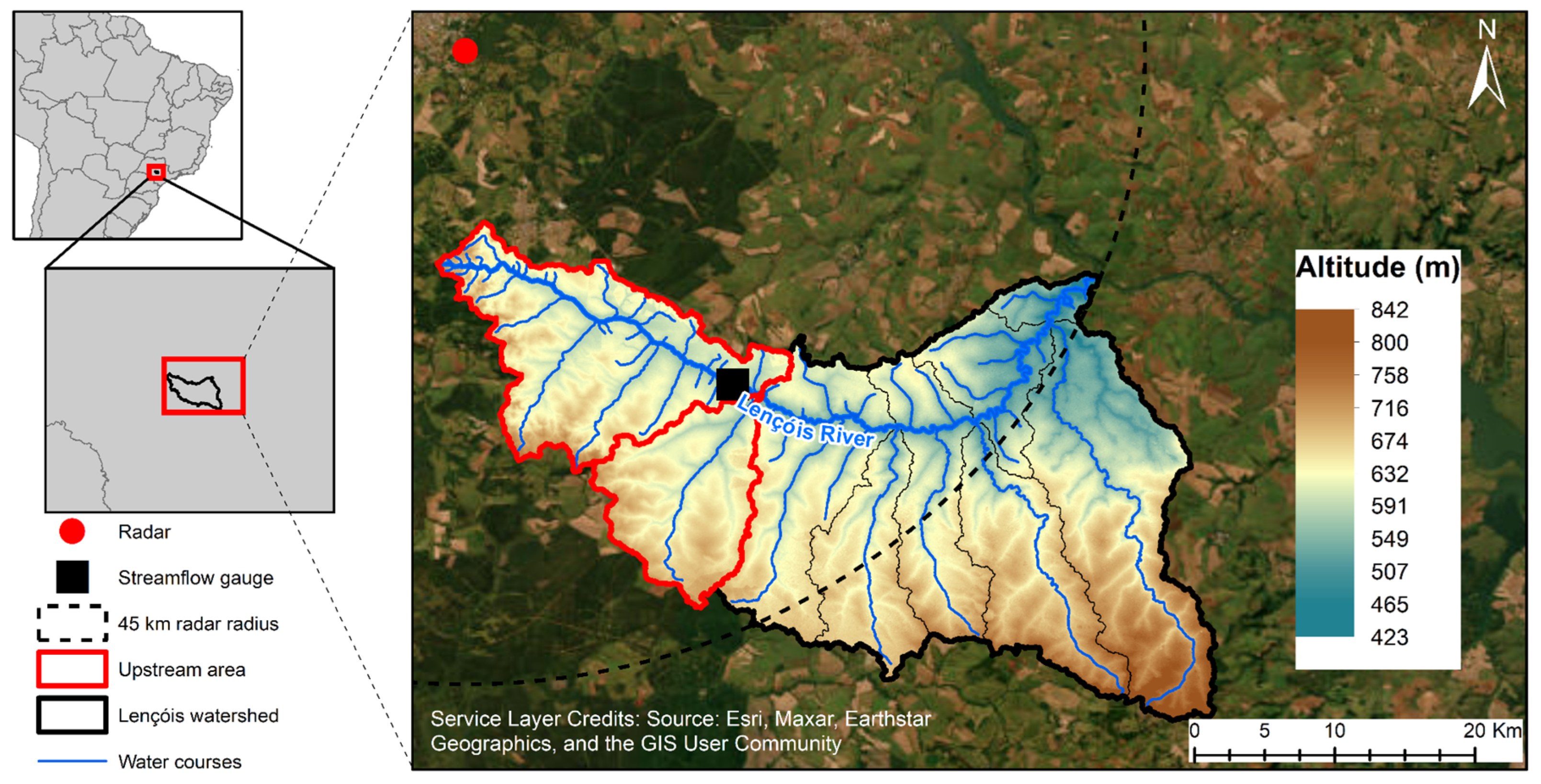
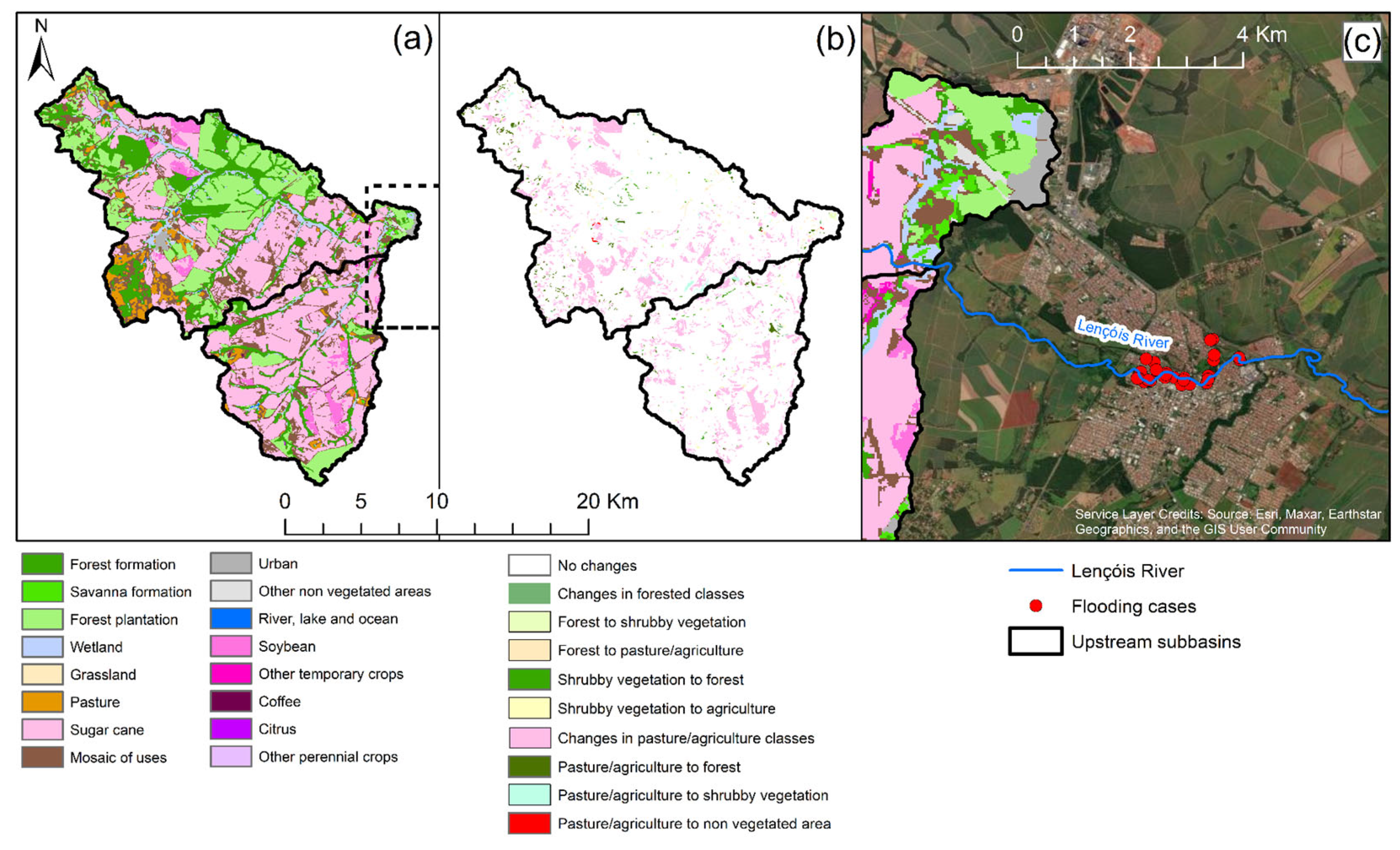
2.1. Study Area

The Lençóis River basin covers an area of 94,855.34 ha and is located in the central region of the state of São Paulo, southeastern Brazil (Figure 1). The river originates in the rural area of Agudos municipality and flows into the Tietê River in the municipality of Igaraçu do Tietê, also extending through the municipalities of Borebi, Lençóis Paulista, the district of Alfredo Guedes, Areiópolis, Macatuba, and São Manuel. Lençóis Paulista is directly influenced by the upstream drainage area of the basin, represented by the sub-basins marked in red in Figure 1.

To assess recent land use cover and its transitions over time, we used Collection 9 of the MapBiomas Project [24], with a 30 m spatial resolution in raster format. For land cover transitions, we analyzed changes from 2016 to 2023, initially identifying 96 transition classes. To improve visualization, we excluded classes with fewer than 100 pixels (30 m × 30 m), representing only 0.4% of the total area, reducing the number of classes to 47. Transitions were then grouped based on major MapBiomas classes: forest, herbaceous and shrubby vegetation, farming, non-vegetated areas, and water. Within each major class (e.g., farming), transitions between subclasses (e.g., coffee to sugarcane) were categorized as “changes in pasture/agriculture classes”, with analogous naming for forests. Transitions across major classes were labeled based on direction, such as “forest to shrubby vegetation”. This classification scheme allowed for representation of transitions in 10 categories shown in Figure 2b.

The upstream sub-watersheds are predominantly rural, with land use primarily for sugarcane cultivation (40%) and forestry (18%) (Figure 2a). Urban areas account for only 0.7% of the total area. From 2016 to 2023 (Figure 2b), 86.5% of the area remained unchanged. The main changes occurred in agricultural areas, involving crop type transitions, accounting for 11% of the total. Other transitions, such as reforestation or deforestation, were marginal, totaling approximately 3%.

Although flood events are reported exclusively in the urban areas of Lençóis Paulista, they tend to occur near the slopes along the Lençóis River, which crosses the city (Figure 2c). In this study, we attribute the river level rise associated with flooding primarily to runoff generated in the upstream watershed. Consequently, surface runoff from the urban drainage network or intense local convective rainfall was not included in the analysis.

2.2. Radar-Based Estimation of Precipitation

The average precipitation volume in the area of interest is obtained from reflectivities measured by the Bauru weather radar, operated by the Institute of Meteorological Research (IPMet). To estimate precipitation, the reflectivities (in dBZ) are initially converted to mm⁶ m⁻³ (Equation (1)). Emídio and Landim [25,26] conducted tests with the Z-R relationships of ref. [27], ref. [28] and Calheiros (personal communication, Equation (2)) to quantify the average rainfall using the Bauru weather radar. Each relationship was compared to a reference of rain gauges interpolated using the Thiessen method. The results indicated that the Calheiros relationship provided the closest estimates to the Thiessen method. The Calheiros relationship (Equation (2)) is a traditional power-law equation of the form Z = aR^b, with coefficients a = 32 and b = 1.65:

$$z={10}^{Z/10}$$

(1)

$$R={\left({\displaystyle \frac{z}{32}}\right)}^{{\displaystyle \frac{1}{1.65}}}$$

(2)

where Z is the radar reflectivity factor in dBZ, z is the radar reflectivity factor in mm⁶ m⁻³, and R is the precipitation rate in mm h⁻¹.

The IPMet radars perform atmospheric scans every seven and a half minutes whenever there is rainfall within their coverage area. We analyzed the precipitation estimates conducted between 2016 and 2024, totaling 332,846 scans. For each scan, five precipitation-related values were extracted: the estimated instantaneous precipitation at the date/time of the scan (ac00h) and the accumulated precipitation over the preceding 12 (ac12h), 24 (ac24h), 36 (ac36h), and 48 (ac48h) hours before the radar scan. To estimate the time series of the average precipitation in the region of interest, we created a mask to represent the area of the two sub-basins of the Lençóis River, which influence flood occurrences in the urban center of Lençóis Paulista (outlined in red in Figure 1).

Due to the Earth’s curvature, S-band weather radars can estimate precipitation volume within a range of up to 240 km. However, because of the angular beamwidth of the electromagnetic signal emitted by the antenna—approximately 2° for the IPMet radar that provided the data used in this study—the spatial resolution degrades significantly with distance. As shown in Figure 1, the studied watershed lies within a 45 km radius of the radar, which is considered an optimal range for S-band weather radars, resulting in a spatial resolution of approximately 1 km at this distance. It is also noteworthy that the watershed is located outside the radar’s blind cone (the region within 5 km of the radar), where precipitation detection is limited due to the elevation angle constraint of the antenna, which, for IPMet radars, reaches a maximum of 45° above the horizon.

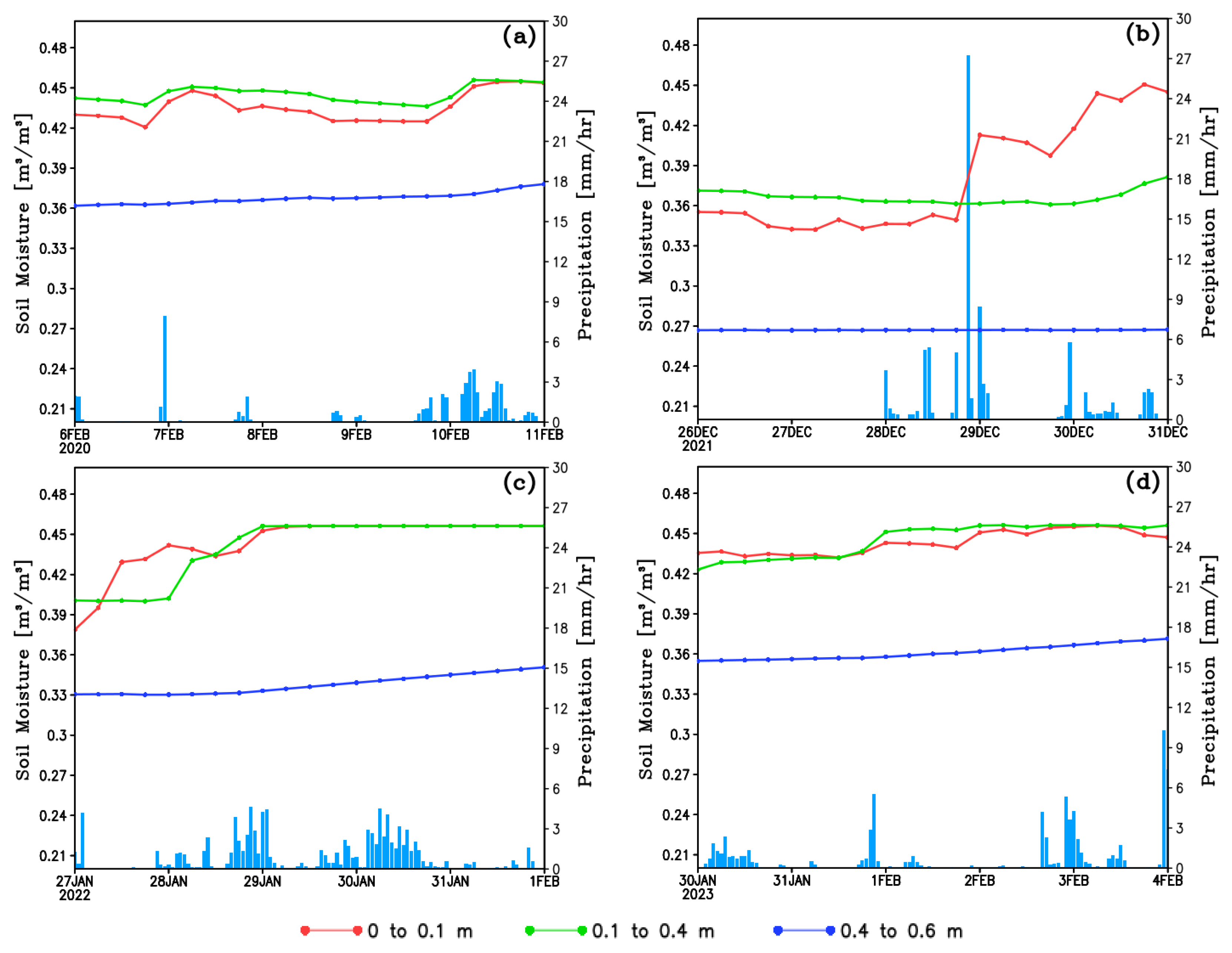
2.3. Soil Moisture Simulation with JULES Model

The soil moisture data are estimated by the surface model JULES (Joint UK Land Environment Simulator [29,30]), which is operationally run at IPMet/Unesp. JULES is driven with incoming solar and longwave radiation, air temperature and specific humidity at 2 m, wind speed at 10 m, and surface atmospheric pressure, all obtained from the Global Forecast System (GFS) atmospheric model. The GFS is a weather forecasting model developed by the National Center for Environmental Prediction (NCEP), affiliated with the National Oceanic and Atmospheric Administration (NOAA), with a spatial resolution of 0.25°. Regarding precipitation, JULES assimilates a field composed of rain gauge data, radar estimates, and satellite estimates [31]. The simulation with the JULES model began in 2015 and has been running daily in a cyclical manner (each model run is initialized with fields simulated on the previous day). The simulated area covers South America almost entirely. The soil moisture estimation field is recorded every 6 h and is publicly available on the IPMet website (https://www.ipmetradar.com.br/ → products → Soil Moisture—accessed on 19 May 2025). As the JULES surface model simulations began in 2015, and as approximately one year of simulation is required for the surface model to warm up, we selected only events/cases that occurred from 2016 onward.

The model simulates soil moisture in three layers: the topmost layer, ranging from 0 to 10 cm in depth (z1), followed by a second layer extending from 10 to 40 cm (z2), and a third layer between 40 and 100 cm (z3).

The spatial resolution of the JULES model (10 km × 10 km) may be too coarse to adequately represent the upstream sub-basins, which cover an area of approximately 300 km² and are therefore represented by only three grid points. Ideally, the model would be forced with higher-resolution analyses than those provided by GFS, in order to obtain more refined soil moisture estimates—although such datasets are not yet readily available for Brazil. However, as noted in Section 2.1, the study area is predominantly agricultural, and thus spatial heterogeneity is not expected to play a critical role in this context.

2.4. Selection of Parameters Used in FPI Calculation

To determine the most suitable parameters for calculating the FPI, analyses of precipitation and estimated soil moisture were conducted for four flood events (Figure 3), including the day of occurrence and the preceding days of each event.

In two of the selected events, soil moisture (SM) conditions were very similar (Figure 3a,d). The soil remained wet in the days leading up to and on the day of the flood, with layer z2 retaining more water than z1 throughout most of the period. This was likely due to previous rainfall that moistened the top two soil layers. The lower SM in z1 compared to z2 can be explained by the evaporation simulated by the model in this layer, which responds more quickly to surface conditions due to its shallow depth. Regarding precipitation, both events showed similar rainfall patterns, although precipitation was less continuous near the event in Figure 3d.

In the event shown in Figure 3b, there was no precipitation in the first two days, keeping soil moisture low. Starting on the 28th, periods of high rainfall occurred throughout the day, with a peak in precipitation at the end of the day. However, this rainfall only moistened the topsoil layer. When precipitation resumed between the 29th and 30th, it continued to wet the surface layer and, to a lesser extent, infiltrate into the second soil layer. The intense rainfall exceeded the soil’s infiltration capacity, leading to high surface runoff in the basin, which ultimately caused the river to overflow.

In Figure 3c, a continuous precipitation pattern can be observed, leading to soil saturation in layers z1 and z2 on the 29th. These layers remained wet in the following days until the flood event, when moisture levels also began to increase in the deeper layer (z3). The saturated soil, combined with well-distributed and continuous precipitation over time, favored surface runoff and, consequently, flooding.

In all flood cases, the days preceding the events were characterized by high soil moisture levels, so that on the days of the floods, soil moisture in layers z1 and z2 was similar, regardless of precipitation intensity.

For future operationalization of this index, we considered the limitation that available soil moisture data are always delayed by one day. For this reason, the FPI uses soil moisture estimates from the 24 h preceding its application.

Based on the presented analyses, precipitation and soil moisture were key variables contributing to the occurrence of floods. By examining Figure 3, it was possible to identify the specific periods that were most relevant to flood events. Consequently, the FPI was calculated considering soil moisture in the first three layers simulated by the JULES model, with the soil moisture at the second level being the estimate from 96 h before the event, in addition to accumulated precipitation over the preceding days.

2.5. Selection of Cases with Flooding

The flood events used in our study were selected based on documentation from the Civil Defense of Lençóis Paulista and the Natural Disaster Database of IPMet (https://www.ipmetradar.com.br/2desastres.php, accessed on 19 May 2025), as well as news reports from media outlets containing photographic records or testimonies confirming the occurrence of flooding. In total, we selected nine cases, which are described in

Table 1. Description of flood events in Lençóis Paulista, SP, according to the Integrated Civil Defense System (SIDEC) or the IPMet Natural Disaster Database (IPMet).

Date	Local Time	Event Description
12 January 2016	22:00	The worst flood of the Lençóis River on record, resulting from an extreme rainfall event of 213 mm in a few hours. More than 1342 people were affected, with 997 left homeless and approximately USD 17 million in losses. Besides the rain, the main causes of the flooding were soil saturation, rupture of dams and reservoirs, and water coming from contour lines (SIDEC).
5 February 2017	19:00	Although it did not rain in the urban area on that day, there was a low-amplitude flood in isolated points of the Lençóis River due to the accumulated precipitation of 197 mm in the 24 h preceding the event (SIDEC).
11 January 2018	14:00	Tree falls, gradual flooding, waterlogging, vehicle damage, and disruptions in electricity and water supply were reported (IPMet). https://sampi.net.br/bauru/noticias/2201287/regional/2018/01/temporal-de-grande-intensidade--testa--o-sistema-antienchentes-em-lencois-paulista (accessed on 19 May 2025).
20 February 2019	14:00	Overflow of rivers and streams, gradual flooding, floods, waterlogging, landslides/cracks/damage to properties, traffic congestion/public road blockage, vehicle damage, flash floods and sudden inundations (IPMET). https://g1.globo.com/sp/bauru-marilia/noticia/2019/02/20/chuva-deixa-ruas-alagadas-em-lencois-paulista.ghtml (accessed on 19 May 2025).
10 February 2020	11:00	Overflowing of rivers and streams, gradual flooding, flash floods, waterlogging, landslides/cracks/damage to properties, traffic congestion/road closures, disruptions in electricity and water supply, erosion/sinkholes, pavement damage, runoff, and sudden flooding were recorded (IPMet). https://jornaloeco.com.br/cotidiano/corrego-corvo-branco-tem-principio-de-alagamento/#google_vignette (accessed on 19 May 2025).
30 December 2021	15:30	Heavy rainfall caused flooding in Vila Contente, Av. Vinte e Cinco de Janeiro, in the city center, and overflowed the Lençóis River at the Service for Water and Sewage (SAAE) yard, on Atílio Frezarin Street in Vila Morumbi, Inácio Anselmo Street, and São Paulo Street in Mamedina (SIDEC).
31 January 2022	02:00	High rainfall observed in Lençóis Paulista and the surroundings, with notable values in Agudos, Borebi, and Lençóis Paulista. Lençóis River level rose slowly throughout the night. At 4:30 AM on 31 January 2022, the Contingency Plan for Floods and Inundations was activated, and the evacuation of properties near the river was carried out (SIDEC).
3 February 2023	22:22	According to the monitoring system, over 70 mm fell in the last few hours, causing runoff, flooding, and water accumulation in various areas. The Civil Defense authorities reported that the Lençóis River remained within its channel, except at more sensitive points. Source: https://jornaloeco.com.br/cidade/chuva-causa-alagamentos-em-regioes-de-lencois-paulista/ (accessed on 19 May 2025).
18 February 2023	18:00	Intense short-duration rainfall (85 mm between 6 PM and 7 PM, with a daily total of 120.6 mm), deficiency in the micro-drainage of stormwater, and overflow of the Corvo Branco stream channel in Vila Contente, as well as the overflow of the Rio Lençóis channel in Jardim Morumbi, Centro, Vila Mamedina, and Vila Repke (SIDEC).

.

2.6. Selection of Cases Without Flooding

In addition to the selected flood events, we developed an objective criterion to identify cases in which the variables of interest (precipitation and soil moisture) were elevated but did not lead to flooding. This procedure is essential for training the index, as such cases could represent false-alarm situations.

Using time series of accumulated precipitation over 48 h, 36 h, 24 h, 12 h, and 0 h (see Section 2.2 for further details), we selected the three highest values for each accumulation period, identifying a total of 15 events of non-flooding. A previous step consists of removing the nine selected flood cases, as well as the five days preceding and following each flood event in the original time series. Then, sequentially, we select a non-flood case, and also remove the five days preceding and following this case, before going to the next non-flood case. This procedure ensures that the tracked non-flood cases were not influenced, even remotely, by flooding events, and that non-flood events are sufficiently far from each other.

Differently from precipitation, there is a maximum value expected for the soil moisture, which is the average porosity in the sub basins. For this reason, we randomly selected three values among the highest ones of metrics 24hz1, 96hz2, 24hz2 and 24hz3, totaling 12 events. The nomenclatures “96 h” and “24 h” refer to the soil moisture 96 and 24 h before a given reference time, and z1, z2 and z3 are the soil layers (see Section 2.3). The procedure of removing the window of five days before and after the flood and non-flood events was also applied to these parameters.

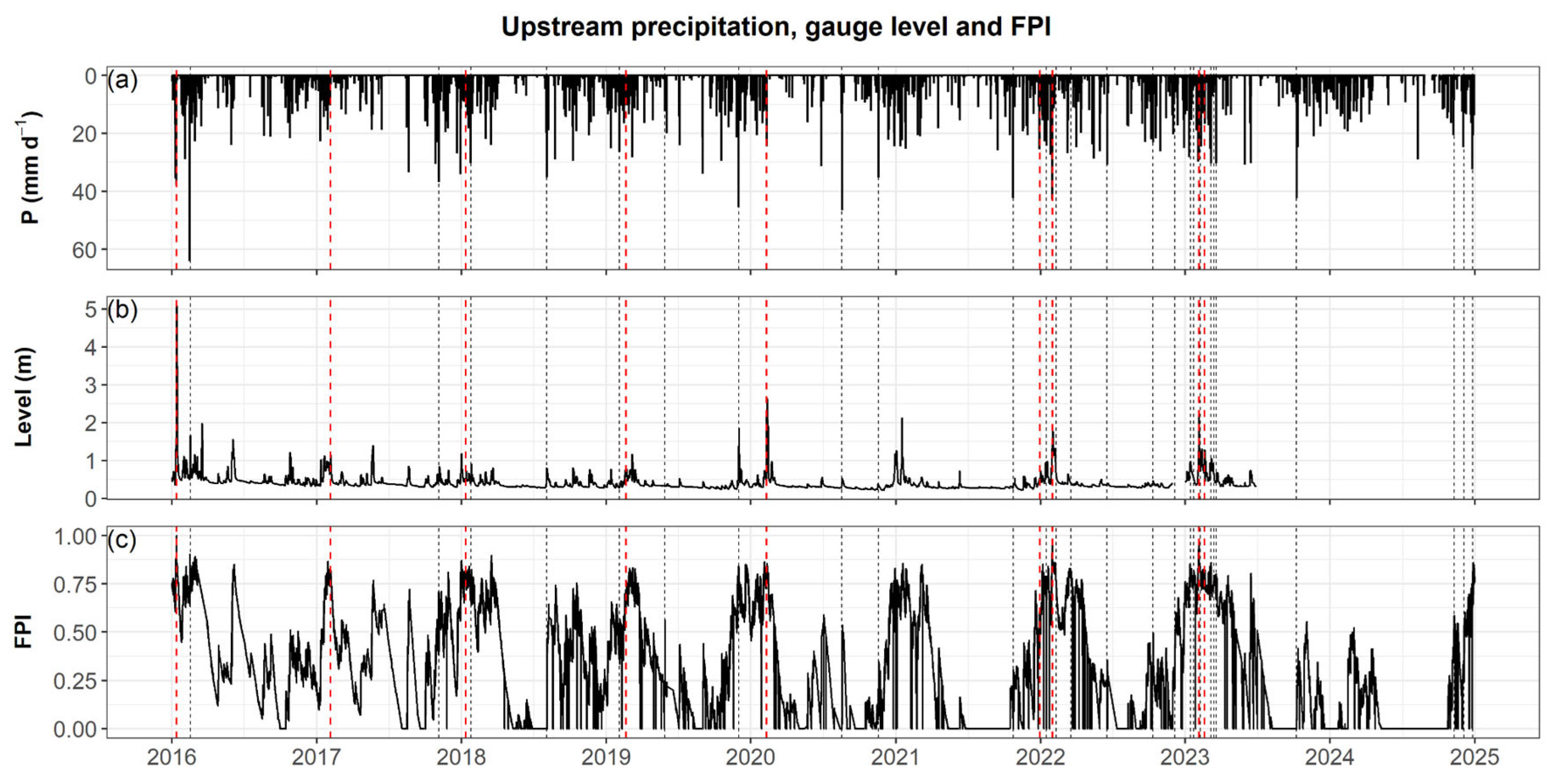
2.7. Flood Probability Index Calculation

With the selected parameters, Equation (3) was proposed for calculating the FPI precursor, which corresponds to the non-normalized index value:

$$\begin{gathered} x_i=a{\displaystyle \frac{{96hz2}_i}{\overline{96hz2}}}+b{\displaystyle \frac{{24hz1}_i}{\overline{24hz1}}}+c{\displaystyle \frac{{24hz2}_i}{\overline{24hz2}}}+d{\displaystyle \frac{{24hz3}_i}{\overline{24hz3}}} \\ +e {\displaystyle \frac{{ac00h}_i}{\overline{ac00h}}}+f{\displaystyle \frac{{ac12h}_i}{\overline{ac12h}}}+g{\displaystyle \frac{{ac24h}_i}{\overline{ac24h}}}+h{\displaystyle \frac{{ac36h}_i}{\overline{ac36h}}}+o{\displaystyle \frac{{ac48h}_i}{\overline{ac48h}}} \end{gathered}$$

(3)

where $x_i$ is the non-normalized FPI; a, b, c, d, e, f, g, h and o are the coefficients that define the weights for each variable; index $i$ represents each event, with 9 flood events and 27 non-flood cases; $z1$, $z2$ and $z3$ correspond to instantaneous soil moisture at depths of 0–0.1 m, 0.1–0.4 m, and 0.4–0.6 m, respectively, and 24 h and 96 h indicate the antecedence in hours to the time that the index is being computed; $ac12$, $ac24$, $ac36$ and $ac48$ represent the accumulated precipitation over the last 12, 24, 36, and 48 h, respectively, while $ac00$ corresponds to the instantaneous precipitation; $\overline{96hz2}$, $\overline{24hz1}$, $\overline{24hz2}$, $\overline{24hz3}$, $\overline{ac00h}$, $\overline{ac12h}$, $\overline{ac24h}$, $\overline{ac36h}$ and $\overline{ac48h}$ are the mean values considering the nine flood events described in Table 1.

The multiplicative coefficients in Equation (3) represent the weights assigned to each term. These coefficients were obtained using a custom numerical method based on a cascading loop structure, in which the coefficients varied incrementally by 0.01, ensuring that their sum always equals 1. This process has a high computational cost, as it requires executing 101⁹ iterations (9 coefficients, each varying from 0 to 1 in increments of 0.01). A machine with an Intel XEON 2.4 GHz processor required 155 h of processing to determine the optimal coefficients for Equation (3) that best represent the FPI.

For each set of coefficients, the algorithm computed the non-normalized FPI value (x_i) for the 9 flood events (Table 1) and for the 27 non-flood cases. Equation (3) shows that the higher the x_i value, the greater the probability of a flood event.

To better represent the Flood Potential Index, we used the normalized FPI (Equation (4)), with values of 0 and 1 corresponding to the minimum (x_min) and maximum (x_max) values of x_i among the 36 analyzed events/cases, respectively:

$${FPI}_i={\displaystyle \frac{ x_i-x_{min}}{x_{max}-x_{min}}}$$

(4)

Subsequently, the FPI values are divided into two sets: one for events that resulted in flooding (FPIsC) and another for those that did not (FPIsS). The values of FPIsC are iteratively compared with those of FPIsS, selecting the coefficients that maximize the difference between these two groups. Specifically, the goal is to maximize the number of cases where FPIsC > FPIsS. If multiple coefficient sets yield the same number of correctly classified events, the one that maximizes the difference between the mean values of FPIsC and FPIsS is selected.

3. Results

Table 2. Mean parameters of the non-normalized index (see Section 2.7 for details). Soil moisture-related parameters are in m³m⁻³, and precipitation-related parameters are in mm h⁻¹.

$\overline{96\mathit{h}\mathit{z}2}$	$\overline{24\mathit{h}\mathit{z}1}$	$\overline{24\mathit{h}\mathit{z}2}$	$\overline{24\mathit{h}\mathit{z}3}$	$\overline{\mathit{a}\mathit{c}00\mathit{h}}$	$\overline{\mathit{a}\mathit{c}12\mathit{h}}$	$\overline{\mathit{a}\mathit{c}24\mathit{h}}$	$\overline{\mathit{a}\mathit{c}36\mathit{h}}$	$\overline{\mathit{a}\mathit{c}48\mathit{h}}$
0.390	0.405	0.392	0.333	6.112	1.361	1.049	1.049	0.755

presents the average parameters of Equation (3) used, considering the mean of the 9 flood events and the 27 selected non-flood cases. It was observed that soil moisture in the second layer remained persistently high in the evaluated cases, with nearly identical values of 0.39 m³m⁻³ at 96 and 24 h before the events/cases, which represents a saturation level of around 85% for these layers. Soil moisture values are higher near the surface and decrease with depth, as typically observed in the infiltration process.

Based on these average parameters, it was possible to calculate the adjusted coefficients of the FPI, as presented in

Table 3. Adjusted FPI coefficients found during the iteration process.

$\mathit{a}$	$\mathit{b}$	$\mathit{c}$	$\mathit{d}$	$\mathit{e}$	$\mathit{f}$	$\mathit{g}$	$\mathit{h}$	o
0.05	0.36	0.53	0.01	0.01	0.02	0.00	0.01	0.01

. We observed that the parameters related to soil moisture contributed with higher weights in the index than those related to precipitation, especially the moisture in the second layer (z2, c = 0.53), followed by the first layer (z1, b = 0.36), both at 24 h in advance.

The unnormalized FPI had a minimum value of 0.668 and a maximum of 1.183 among our sample of cases. After applying the normalization (Equation (4)), the FPI for the flood cases is presented in

Table 4. FPI calculated for cases with flood.

Date	FPI
12 January 2016	1.000
5 February 2017	0.818
11 January 2018	0.771
20 February 2019	0.662
10 February 2020	0.824
30 December 2021	0.567
31 January 2022	0.902
3 February 2023	0.961
18 February 2023	0.833

.

Notably, the flood event with the highest FPI occurred on 12 January 2016, with FPI = 1, while the lowest occurred on 30 December 2021, with FPI = 0.567. In particular, the 2016 flood was the worst ever recorded, and the maximum index assigned to this event suggests that FPI magnitude can be used as a measure of flood severity, as we will discuss later. It is also worthy to note that all flood cases were in the austral summer.

Using the coefficients obtained from both flood and non-flood cases, we extrapolated the index to the entire available time series, covering the period from 2016 to 2024 (Figure 4). We observed that the FPI (Figure 4c) exhibits a consistent seasonal variation, with higher values during the rainy season (Figure 4a), generally exceeding 0.7, except in 2024. Alternatively, lower values of the index, typically below 0.2, are observed during the dry season.

Additionally, we noted that, in general, the index responds to rainfall events throughout the year, not only during the rainy season. However, in some cases, the FPI remains at zero. In these instances, despite the occurrence of rainfall, soil moisture was sufficiently low that the entire precipitation amount was absorbed through infiltration.

Furthermore, the water level of the Lençóis River, measured upstream of the city of Lençóis Paulista (Figure 4b), is correlated with the FPI (r = 0.52, p < 2.2 × 10⁻¹⁶). In the most severe case, in 2016, the river level exceeded 5 m, leading to the overflow of the main channel. In addition to this event, the flood cases of 2020, 2022, and 18 February 2023 were also captured as local maxima in the river level time series. However, as shown in Figure 1, this gauge only covers the drainage area of the sub-basin nearest to the headwaters, thus not accounting for the contribution of the second sub-basin.

Using the entire time series of FPI values as a reference—including those in Table 4 but excluding the 5-day periods before and after the nine flood cases—it was possible to classify the probability indices according to the likelihood of flood occurrence for the city of Lençóis Paulista (

Table 5. Chance of flooding according to the Flood Probability Index (FPI) applied to Lençóis Paulista.

Threshold	Chance of Flooding	Occurrence of Events/Cases
		Events of Flooding	All Cases Outside Flood Periods
FPI $<$ 0.563	Low	0% (0 events)	70% (219,369 cases)
0.563 $\le$ FPI $<$ 0.783	Moderate	33% (3 events)	25% (78,517 cases)
0.783 $\le$ FPI $<$ 0.905	High	44% (4 events)	5% (15,784 cases)
FPI $\ge$0.905	Very high	22% (2 events)	0.0% (0 cases)

). This approach allowed us to assign a qualitative dimension to flood risk.

We determined the threshold for the “very high” category based on the FPI value above which no non-flood cases occurred. For the other classification ranges, we defined the “high”, “moderate”, and “low” categories as those containing 5%, 25%, and 70% of all cases outside flood periods, respectively.

Based on this classification, the events on 11 January 2018, 20 February 2019, and 30 December 2021 were categorized as moderate probability, while those on 5 February 2017, 10 February 2020, 31 January 2022, and 18 February 2023 were classified as high probability. The events on 12 January 2016 and 3 February 2023 were classified as very high probability.

To better understand how the classification in Table 5 and the FPI respond to variations in soil moisture across different layers, we present a scatter plot of FPI against the respective soil moisture parameters (Figure 5). Beginning with the uppermost layer (US24_z1), we observed a positive relationship in which FPI increases with rising soil moisture, suggesting the presence of a minimum threshold of approximately 0.22 m³/m³ for FPI values to exceed zero. It is also noteworthy that the data exhibit considerable dispersion, indicating that even relatively high soil moisture levels may result in zero FPI values when not accompanied by a specific combination of other influencing parameters.

For the intermediate layer, represented by the 24 h average (US24h_z2), the dispersion is the lowest among all soil moisture parameters in relation to FPI. This finding is consistent with the highest coefficient observed in Table 3. An interesting feature in this layer is the presence of vertically aligned data points near the porosity value, also visible in the z1 layer, likely reflecting the effect of accumulated precipitation. In this region, the horizontal dashed line delineates FPI values associated with high to very high flood risk. This highlights that while soil moisture appears to be the primary driver of FPI—particularly at higher, more sensitive thresholds—accumulated precipitation also plays a crucial role.

In contrast, for the deepest layer (US24h_z3), the data show the highest dispersion, and the relationship between soil moisture and FPI is less apparent. This observation is again consistent with the near-zero coefficient associated with this parameter in Table 3. Finally, regarding the 96 h average moisture in layer z2 (US96h_z2), the pattern is similar to that observed for US24h_z2, though with a different contribution that reflects the broader soil moisture profile. Although US24h_z2 emerges as the dominant factor influencing FPI, moisture redistribution following water infiltration into the soil can occur gradually and may thus be more effectively captured by the US96h_z2 parameter.

4. Discussion

The relatively low weights for the parameters related to accumulated precipitation are likely due to two reasons: (i) soil near saturation contributed more significantly to flood events than precipitation magnitude, and (ii) accumulated precipitation over the analyzed time intervals is covariant with soil moisture, explaining similar variances.

An immediate consequence for the selected cases would be to simplify the index using only the first three terms of Equation (3) without significant performance loss. However, the accumulated precipitation seems to have contributed especially to the higher values of FPI, where the transition of classes of flooding is thinner. Caution is also needed when proposing this simplification globally, as the number of flood events analyzed was relatively small and was primarily influenced by the good performance of the JULES model in simulating soil moisture conditions. In cases where the land surface model has questionable skill, using accumulated precipitation as a proxy for soil moisture is a viable alternative.

Moreover, in other catchments with lower infiltration capacity, runoff generation due to precipitation excess is likely a relevant process, meaning that parameters e, f, g, h, and o should assume higher weights.

Despite the simplicity of the methodology and the consistent results presented, we acknowledge that our approach has some limitations.

The radar itself introduces a source of uncertainty as it often underestimates the precipitation measured in rain gauges [32], due to its limitations in capturing convective systems that produce short but intense rainfall events between scans. Extremely localized rainfall events may not be effectively captured by the FPI, as the index relies on spatial averages that smooth out precipitation patterns. However, we believe that our methodology benefits from the fact that weather radars accurately capture the occurrence and spatial distribution of rainfall. In hydrological modeling, for example, underestimation of precipitation can more critically affect the simulation of physical processes, potentially leading to an implausible set of model parameters.

Moreover, as expected in parsimonious approaches such as the one adopted in this study, the simplicity of the selected parameters does not allow for a spatial characterization of the basin. This limits both the comparison with neighboring basins with different characteristics and the ability to simulate the underlying physical processes. For example, a study conducted in Sweden [33] concluded that among various watershed descriptors, steeper slopes and higher drainage density are generally the most influential factors controlling flood risk. Although the use of spatial averages of rainfall and soil moisture does not allow for the identification of specific areas within the basin that generate higher surface runoff, as is possible with lumped hydrological models, we believe that the relatively small proportion of forested areas compared to those used for agriculture and livestock does not impose a markedly heterogeneous pattern on the basin.

Finally, we assumed that land use changes based on Figure 2b were minimal and that FPI variability was driven solely by climate variations. However, in 2020, flood mitigation measures were implemented in the city, including the lowering of 14 reservoirs, increasing flood detention capacity from 1.1 million to 1.3 million m³, and enhancing the Lençóis River’s diversion capacity from 245,000 to 350,000 m³ h⁻¹ (https://jornaloeco.com.br/cidade/apos-cinco-anos-de-enchente-historica-prevencao-e-palavra-de-ordem-em-lencois/, accessed on 19 May 2025). As a result, since 2021, floods have been expected to occur only at higher FPI values, which may explain the absence of flooding in early 2021 and late 2024, despite FPI values exceeding 0.85 (Figure 4).

Lastly, the relatively short analysis period allowed us to use only nine flood events. To strengthen our analysis with a larger sample, we extrapolated the FPI to the entire study period, which ultimately led to the development of the classification in Table 5.

Given these findings and the importance of anticipating flood events, we intend to implement an operational system for real-time FPI determination, allowing the index to be calculated as soon as the radar completes its volumetric scan. Once fully operational and publicly available, the FPI will serve as a valuable tool for forecasting and informing the population about potential floods, enabling proactive measures to minimize damage and save lives. In the context of climate change, the index could also be computed under projected rainfall scenarios for the coming decades as an impact assessment tool, supporting the development of adaptation strategies.

Evidently, other alternatives based on nature-based solutions are important tools in the context of flooding adaptation. For example, pasture restoration practices—such as plowing, reseeding, and drainage—reduce the natural variability of moisture patterns in the surface soil layer when compared to adjacent undisturbed areas, thereby contributing to flood risk reduction [34].

5. Conclusions

By evaluating several cases of flood occurrence and non-occurrence, we identified the hydrometeorological variables that effectively influenced flooding events in Lençóis Paulista, São Paulo, Brazil, enabling the proposal of a novel index, the FPI.

Soil moisture conditions in different layers prior to each event stood out over accumulated precipitation variables in the index calculation for the selected events. This result suggests that excess saturation, rather than precipitation intensity, was the primary runoff-generating mechanism leading to the observed floods. The relatively low contribution of rainfall can be attributed to either a basin with high infiltration capacity or underestimation of rainfall volumes by the radar. However, in the upper distribution of FPI, the rainfall played an important role in dividing cases of high and very high chance of flooding.

Of the flood events, 33% (three cases in nine cases) were classified as moderate-risk, meaning they had a relatively low FPI, ranging between 0.563 and 0.783. In 25% of the non-flood cases (78,517), the classifications indicated moderate flood risk. This can be explained by inaccuracies in precipitation and soil moisture estimates. Therefore, more precise FPIs could be obtained if real-time rainfall and soil moisture measurements were available at certain points in the basin and were operationally incorporated into the index calculation.

It is important to emphasize that the FPI is not based on strict physical processes of water transport in the soil, as is the case with hydrological models. This means that for different regions—with varying slopes and drainage networks—the coefficients used in the FPI must be recalibrated based on past flood events in each specific location. This is because the rainfall patterns and precipitation accumulations that triggered floods in Lençóis Paulista are unlikely to be the same as those responsible for flooding in other areas. In this sense, the FPI is determined through qualitative rather than absolute (calibrated) effects of soil moisture.

Despite its simplicity, the system used in this study has the potential to be operationalized for real-time flood risk forecasting based on established thresholds and could be used by agencies such as Civil Defense for strategic planning in areas with characteristics similar to those of the studied area. Furthermore, FPI magnitude can be used as a measure of flood severity as well.

For future research, we recommend applying this methodology to different hydrographic regions, preferably in areas with a denser rain gauge network and soil moisture to reduce uncertainties associated with radar-based precipitation and model estimates. Furthermore, these measurements must be incorporated into the FPI calculation in real time.

References

1. Pörtner, H.-O.; Roberts, D.C.; Tignor, M.; Poloczanska, E.; Mintenbeck, K.; Alegría, A.; Craig, M.; Langsdorf, S.; Löschke, S.; Möller, V. Working Group II Contribution to the Sith Assessment Report of the Intergovernmental Panel on Climate Change. In IPPC 2022: Climate Change 2022: Impacts, Adaptation and Vulnerability; Cambridge University Press: Cambridge, UK, 2022. [Google Scholar]
2. Collischonn, E. Inundações Em Venâncio Aires/RS: Interações Entre as Dinâmicas Natural e Social Na Formação de Riscos Socioambientais Urbanos. Ph.D. Thesis, Universidade Federal de Santa Catarina, Florianópolis, Brazil, 2009. [Google Scholar]
3. Silvestro, F.; Rossi, L.; Campo, L.; Parodi, A.; Fiori, E.; Rudari, R.; Ferraris, L. Impact-Based Flash-Flood Forecasting System: Sensitivity to High Resolution Numerical Weather Prediction Systems and Soil Moisture. J. Hydrol. 2019, 572, 388–402. [Google Scholar] [CrossRef]
4. de Oliveira Silva, L.A.; Castro, J.F.M.; Bueno, G.T. Fatores Intensificadores Das Enchentes/Inundações No Médio e Baixo Rio Piranga–MG. CLIMEP-Climatol. Estud. Paisag. 2016, 9, 18–41. [Google Scholar]
5. Collischonn, W.; Dornelles, F. Hidrologia Para Engenharia e Ciências Ambientais; Associação Brasileira de Recursos Hídricos, ABRHidro: Porto Alegre, Brazil, 2013; 336p. [Google Scholar]
6. Ye, S.; Wang, J.; Ran, Q.; Chen, X.; Liu, L. The Relative Importance of Antecedent Soil Moisture and Precipitation in Flood Generation in the Middle and Lower Yangtze River Basin. Hydrol. Earth Syst. Sci. Discuss. 2021, 2021, 1–35. [Google Scholar]
7. Yu, T.; Ran, Q.; Pan, H.; Li, J.; Pan, J.; Ye, S. The Impacts of Rainfall and Soil Moisture to Flood Hazards in a Humid Mountainous Catchment: A Modeling Investigation. Front. Earth Sci. 2023, 11, 1285766. [Google Scholar] [CrossRef]
8. Kidd, C.; Huffman, G. Global Precipitation Measurement. Meteorol. Appl. 2011, 18, 334–353. [Google Scholar] [CrossRef]
9. Adilson Moreira, I.; Moro Mine, M.; Pereira Filho, A. Modelagem Hidrológica Chuva-Vazão Com Dados de Radar e Pluviômetros. Ing. Agua 2007, 14, 83–96. [Google Scholar] [CrossRef]
10. Wilson, J.W.; Crook, N.A.; Mueller, C.K.; Sun, J.; Dixon, M. Nowcasting Thunderstorms: A Status Report. Bull. Am. Meteorol. Soc. 1998, 79, 2079–2099. [Google Scholar] [CrossRef]
11. Drumond, R.A.S.; Almeida, R.P.; de Nascimento, N.O. Mudanças Climáticas e Plano Diretor: Mitigação de Inundações Em Belo Horizonte. Cad. Metrópole 2023, 25, 899–922. [Google Scholar] [CrossRef]
12. Ferreira, M.J.; da Rocha, H.R. Green Roof Infrastructure Outperforms Grey Technology in Flood Mitigation in São Paulo’s Urbanized Region. Front. Built Environ. 2023, 9, 1254942. [Google Scholar] [CrossRef]
13. dos Santos, F.M.; de Souza Pelinson, N.; de Oliveira, R.P.; Di Lollo, J.A. Using the SWAT Model to Identify Erosion Prone Areas and to Estimate Soil Loss and Sediment Transport in Mogi Guaçu River Basin in Sao Paulo State, Brazil. Catena 2023, 222, 106872. [Google Scholar] [CrossRef]
14. Lopes, T.R.; Folegatti, M.V.; Duarte, S.N.; Zolin, C.A.; Junior, L.S.F.; Moura, L.B.; Oliveira, R.K.; Santos, O.N.A. Hydrological Modeling for the Piracicaba River Basin to Support Water Management and Ecosystem Services. J. S. Am. Earth Sci. 2020, 103, 102752. [Google Scholar] [CrossRef]
15. Domingues, L.M.; de Abreu, R.C.; da Rocha, H.R. Hydrologic Impact of Climate Change in the Jaguari River in the Cantareira Reservoir System. Water 2022, 14, 1286. [Google Scholar] [CrossRef]
16. Tramblay, Y.; Bouaicha, R.; Brocca, L.; Dorigo, W.; Bouvier, C.; Camici, S.; Servat, É. Estimation of Antecedent Wetness Conditions for Flood Modelling in Northern Morocco. Hydrol. Earth Syst. Sci. 2012, 16, 4375–4386. [Google Scholar] [CrossRef]
17. Seiler, R.; Hayes, M.; Bressan, L. Using the Standardized Precipitation Index for Flood Risk Monitoring. Int. J. Climatol. 2002, 22, 1365–1376. [Google Scholar] [CrossRef]
18. Popa, M.C.; Peptenatu, D.; Drăghici, C.C.; Diaconu, D.C. Flood Hazard Mapping Using the Flood and Flash-Flood Potential Index in the Buzău River Catchment, Romania. Water 2019, 11, 2116. [Google Scholar] [CrossRef]
19. Rosmadi, H.; Ahmed, M.; Mokhtar, M.; Lim, C. Reviewing Challenges of Flood Risk Management in Malaysia. Water 2023, 15, 2390. [Google Scholar] [CrossRef]
20. Bang, H.N.; Burton, N.C. Contemporary Flood Risk Perceptions in England: Implications for Flood Risk Management Foresight. Clim. Risk Manag. 2021, 32, 100317. [Google Scholar] [CrossRef]
21. Lee, H.; Calvin, K.; Dasgupta, D.; Krinner, G.; Mukherji, A.; Thorne, P.; Trisos, C.; Romero, J.; Aldunce, P.; Barrett, K. Climate Change 2023: Synthesis Report. Contribution of Working Groups I, II and III to the Sixth Assessment Report of the Intergovernmental Panel on Climate Change; The Australian National University: Canberra, Australia, 2023; ISBN 92-9169-164-X. [Google Scholar]
22. Chitwatkulsiri, D.; Miyamoto, H. Real-Time Urban Flood Forecasting Systems for Southeast Asia—A Review of Present Modelling and Its Future Prospects. Water 2023, 15, 178. [Google Scholar] [CrossRef]
23. Ringo, J.; Sabai, S.; Mahenge, A. Performance of Early Warning Systems in Mitigating Flood Effects. A Review. J. Afr. Earth Sci. 2024, 210, 105134. [Google Scholar] [CrossRef]
24. Souza, C.M., Jr.; Shimbo, J.Z.; Rosa, M.R.; Parente, L.L.; Alencar, A.A.; Rudorff, B.F.; Hasenack, H.; Matsumoto, M.; Ferreira, L.G.; Souza-Filho, P.W. Reconstructing Three Decades of Land Use and Land Cover Changes in Brazilian Biomes with Landsat Archive and Earth Engine. Remote Sens. 2020, 12, 2735. [Google Scholar] [CrossRef]
25. de Oliveira Emídio, Z.P. Impacto Do Balanço Hídrico Em Diferentes Tipos de Solos: Comparação Entre Dados de Radar-Pluviômetro e Análise de Tendência Da Chuva Média Em Área Agrícola. Ph.D. Thesis, Universidade Estadual Paulista (Unesp), Rio Claro, Brazil, 2008. [Google Scholar]
26. Emidio, Z.P.; Landim, P.M.B. Análise de superfície de tendência aplicada à chuva medida por radar meteorológico nas regiões de Assis e Piracicaba, SP. Geociências 2008, 27, 439–449. [Google Scholar]
27. Marshall, J.S.; Langille, R.C.; Palmer, W.M.K. Measurement of Rainfall by Radar. J. Meteorol. 1947, 4, 186–192. [Google Scholar] [CrossRef]
28. Jones, D.M.A. Rainfall Drop-Size Distribution and Radar Reflectivity; Urban Meteorology Laboratory, State Water Survey: Urbana, IL, USA, 1956; pp. 1–20. [Google Scholar]
29. Best, M.J.; Pryor, M.; Clark, D.B.; Rooney, G.G.; Essery, R.L.H.; Ménard, C.B.; Edwards, J.M.; Hendry, M.A.; Porson, A.; Gedney, N.; et al. The Joint UK Land Environment Simulator (JULES), Model Description—Part 1: Energy and Water Fluxes. Geosci. Model Dev. 2011, 4, 677–699. [Google Scholar] [CrossRef]
30. Clark, D.B.; Mercado, L.M.; Sitch, S.; Jones, C.D.; Gedney, N.; Best, M.J.; Pryor, M.; Rooney, G.G.; Essery, R.L.H.; Blyth, E.; et al. The Joint UK Land Environment Simulator (JULES), Model Description—Part 2: Carbon Fluxes and Vegetation Dynamics. Geosci. Model Dev. 2011, 4, 701–722. [Google Scholar] [CrossRef]
31. Borges, I.V.G.; Moreira, D.S.; Rozante, J.R. Precipitation Field from Rainfall Measurements and Rainfall Estimates from IPMet’s Radars. Anuário Inst. Geociências-UFRJ 2019, 42, 417–426. [Google Scholar] [CrossRef]
32. Schleiss, M.; Olsson, J.; Berg, P.; Niemi, T.; Kokkonen, T.; Thorndahl, S.; Nielsen, R.; Ellerbæk Nielsen, J.; Bozhinova, D.; Pulkkinen, S. The Accuracy of Weather Radar in Heavy Rain: A Comparative Study for Denmark, the Netherlands, Finland and Sweden. Hydrol. Earth Syst. Sci. 2020, 24, 3157–3188. [Google Scholar] [CrossRef]
33. Ahlmer, A.-K.; Cavalli, M.; Hansson, K.; Koutsouris, A.J.; Crema, S.; Kalantari, Z. Soil Moisture Remote-Sensing Applications for Identification of Flood-Prone Areas along Transport Infrastructure. Environ. Earth Sci. 2018, 77, 533. [Google Scholar] [CrossRef]
34. Wallace, E.E.; Chappell, N.A. A Statistical Comparison of Spatio-temporal Surface Moisture Patterns beneath a Semi-natural Grassland and Permanent Pasture: From Drought to Saturation. Hydrol. Process. 2020, 34, 3000–3020. [Google Scholar] [CrossRef]
Figure 1. Study area. Left: Map of South American continent and location of the Lençóis River basin in relation to Brazil and the state of São Paulo. Right: Lençóis River basin (area outlined in black), highlighting the upstream sub-basins of the city of Lençóis Paulista (outlined in red). The color scale represents the altitude within the basin in meters, while the external area is depicted with satellite imagery. The IPMet radar (red dot) is located in the NW part of the domain, with the 45 km radar radius shown by the dashed line. DAEE 5D-013 streamflow/level gauge is represented by the black square.
Atmosphere 16 00633 g001
Figure 2. Land use map of the upstream sub-basins of the urban area of Lençóis Paulista for the year 2023 (a), land cover transitions from 2016 to 2023 (b), and a zoomed-in view of the region outlining the sub-basins and the beginning of the urban area (c). The red points in (c) indicate the locations of the events described in Table 1. The dashed line represents the area in (a) shown in (c).
Atmosphere 16 00633 g002
Figure 3. Time series of average soil moisture (lines, in m3 m−3) and precipitation estimates from the Bauru radar (blue bars, in mm h−1) for the studied basin, corresponding to the flood events on (a) 10 February 2020, (b) 30 December 2021, (c) 31 January 2022, and (d) 3 February 2023. Soil moisture is presented at three depth levels: z1, from 0 to 0.1 m (red curve); z2, from 0.1 to 0.4 m (green curve); and z3, from 0.4 to 1.0 m (blue curve).
Atmosphere 16 00633 g003
Figure 4. Time series of (a) average precipitation (mm d−1) in the sub-basins of the Lençóis River upstream of the city of Lençóis Paulista; (b) Lençóis River water level at station 5D-013 (see Figure 1), in meters; and (c) the calculated FPI. The red and gray dotted lines represent the dates of flood and non-flood events, respectively, used to estimate the FPI parameters.
Atmosphere 16 00633 g004
Figure 5. Scatterplot of FPI (y-axis) versus the soil moisture parameters US96h_z2, US24h_z1, US24h_z2 and US24h_z3 (x-axis), in m3m−3. Red dashed lines represent the thresholds described in Table 5 for chance of flooding. Coefficient of determination considering a linear fit between FPI and parameters are US96h_z2 (R2: 0.84, p < 2.2 × 10⁻¹⁶), US24h_z1 (R2: 0.77, p < 2.2 × 10⁻¹⁶), US24h_z2 (R2: 0.92, p < 2.2 × 10⁻¹⁶), and US24h_z3 (R2: 0.36, p < 2.2 × 10⁻¹⁶).
Atmosphere 16 00633 g005