Revealing Emission Patterns of Urban Traffic Flows: A Complex Network Theory Perspective

Abstract

Traffic emissions resulting from vehicle travel across origin–destination (OD) pairs pose significant challenges to sustainable urban development, necessitating a systematic understanding of emission patterns to inform effective mitigation policies. Existing studies often focus on the locations where emissions occur, overlooking emission flows between OD pairs, which could lead to incomplete policy formulation. This study proposes a new emission pattern analysis framework. Specifically, we construct the Urban Traffic Emission Flow Network (UTEFN) based on comprehensive individual vehicle data, and then systematically analyze its spatiotemporal characteristics and network structure by using complex network theory. Our findings show that the node weighted degree captures emissions attributable to specific nodes, revealing that critical emission sources may be overlooked in traditional analyses. Edge weights identify high-emission OD edges and associated travel behaviors. Furthermore, the emission distributions for different vehicle types and gases exhibit heavy-tailed scaling laws, indicating that emission reduction policies targeting a few key nodes or edges could impact a notable proportion of traffic emissions. In structural analysis, community detection revealed distinct clusters of emission flows, with the formation of high-emission communities associated with specific spatial configurations and travel behaviors. The findings provide valuable insights into strategic planning for clean traffic systems and urban emission reduction.

1. Introduction

Traffic emissions represent a major risk to climate stability and public health. The transportation sector was responsible for approximately one-fourth of global carbon emissions in 2022, according to data reported by the International Energy Agency [1]. Moreover, traffic emissions contribute to ambient air pollution, increasing risk levels for multiple diseases and the incidence of premature mortality [2,3]. Therefore, urban traffic emissions have become a widespread concern [4].

Urban traffic emission patterns are the aggregated characteristics of individual vehicle emission patterns and provide effective information to support emission reduction policies [5]. The analysis of urban traffic emission patterns typically involves two stages: emission quantification and characterization.

Quantification methods are categorized into “top-down” and “bottom-up” approaches. Top-down approaches estimate emissions via aggregated data, such as traffic yearbooks [6,7,8]. However, the lack of vehicle travel data renders these estimates imprecise [9]. Therefore, recent studies tend to use bottom-up approaches [10,11,12]. Bottom-up approaches quantify emissions on the basis of individual vehicle travel data, offering a more accurate reflection of emission patterns. Nonetheless, the implementation of bottom-up approaches faces major challenges due to the difficulty of gathering comprehensive vehicle travel data.

Comprehensive vehicle travel data require four key attributes that are challenging to fulfill: a complete classification of vehicle types, detailed parameter information, extensive spatiotemporal coverage, and high sampling rates. Existing studies mainly acquire such travel data through GPS devices. However, GPS data are often limited to single vehicle types, e.g., taxis [13], light-duty private vehicles (cars) [14], trucks [15], and buses [16]. Moreover, even for the same vehicle type, variations in vehicle parameters such as fuel type, weight, and emission standards can cause the emission factors to vary dramatically [17]. To overcome these data limitations, researchers have conducted sampling surveys to estimate vehicle types and parameter information. Sun et al. [18] used sampling surveys to infer the fleet compositions on 536 roads via survey data from 40 roads. However, the sampling survey method has small spatiotemporal coverage and high uncertainty. Some studies use intelligent transportation systems to increase the spatiotemporal coverage and sample rate. Zhang et al. [19] utilized radio-frequency identification (RFID) detectors to create a precise vehicle emission inventory for Nanjing. However, the use of RFID systems in cities remains limited. In contrast to these approaches, traffic cameras equipped with automatic license plate recognition (ALPR) play a central role in traffic monitoring and are widely implemented in many cities [20,21,22]. Li et al. [23] used ALPR data to detect all vehicles on an urban road but did not track detailed individual vehicle travel data. Therefore, an emission quantification framework based on camera data for collecting comprehensive individual vehicle travel data is needed.

Regarding the characterization of emissions, existing studies have predominantly concentrated on spatiotemporal characteristics and agglomeration based on the locations where emissions occur, such as grids or road segments. Spatiotemporal characteristics are used to examine how emissions are distributed in time and space. From a temporal perspective, research has primarily addressed variations between weekdays and weekends and between peak and off-peak hours. Dai et al. [24] reported that urban traffic emissions are higher on weekdays than on weekends and holidays. Teng et al. [25] found that there are large differences in emissions during different periods of the day. Therefore, emission reduction policies should focus on weekday emission patterns, especially during peak emission periods. From a spatial perspective, existing studies focus on the hierarchical spatial differentiation of emissions using discrete grids or road segments [26,27]. Moreover, some studies have further revealed the scaling laws and agglomeration of urban traffic emissions. Böhm et al. [14] demonstrated that emission distributions along road segments in three European cities conform to a heavy-tailed distribution function. Cheng et al. [28] reported that high–high agglomeration of truck emissions is mainly distributed outside the sixth-ring roads of Beijing.

However, since traffic emissions are generated by vehicles traveling from a specific origin (O) to a specific destination (D), focusing solely on emission occurrence locations may limit the variety of emission reduction policies that can be formulated. For example, Deng et al. [29] and Tang et al. [30] reported that vehicle restriction policies for specific areas led to longer detours. When high-emission segments are restricted, vehicles circumvent these restrictions by detouring, still completing their travels between the predetermined OD pairs but weakening the expected emission reduction effect of the policies. Therefore, to develop more comprehensive emission reduction strategies, policymakers should also analyze emission patterns from the perspectives of the origins, the destinations, and the interconnections of vehicle travel between OD pairs.

Complex network models are valuable tools for studying interconnected systems and have become a very popular interdisciplinary research method [31,32,33]. By modeling nodes and the flows of elements along edges based on complex network theory, researchers can gain deeper insights into the inherent dynamics and structural characteristics of these systems. In urban traffic systems, vehicles establish spatial interactions between OD pairs, forming emission flows that are inherently linked to travel flows. Therefore, by translating the origin, destination, and emission flows into a directed weighted graph and analyzing their spatiotemporal characteristics and network structure through complex network theory, policymakers can gain new perspectives and insights into the emission pattern formed by interconnected travel flows.

However, the application of complex network analysis to urban emission patterns is still relatively rare.

In summary, the network perspective focuses on the emission flows between different locations rather than just the locations where emissions occur. However, certain challenges have not been adequately addressed: (1) researchers have not determined how to obtain comprehensive vehicle travel data, which is pivotal for quantifying urban traffic emission flows and accurately revealing emission patterns; and (2) detailed studies on the application of the network perspective to urban traffic emission patterns are still very scarce. To address these issues, a methodological framework is introduced in this study. Initially, on the basis of an ALPR system, a comprehensive individual vehicle emission dataset was constructed via a bottom-up approach. This dataset was used to create the Urban Traffic Emission Flow Network (UTEFN), which is adapted to various vehicle models. Additionally, by applying network indicators, we examined the emission characteristics and network structure of the UTEFN and explored potential strategies for reducing urban traffic emissions.

The subsequent sections of the paper are as follows: Section 2 provides an overview of the methodologies employed. Section 3 examines the emission characteristics, while Section 4 investigates the structural characteristics of the UTEFN. Section 5 highlights the key findings, discusses relevant practical implications, and addresses associated uncertainties and limitations. Section 6 summarizes the conclusions of this study.

2. Methodologies

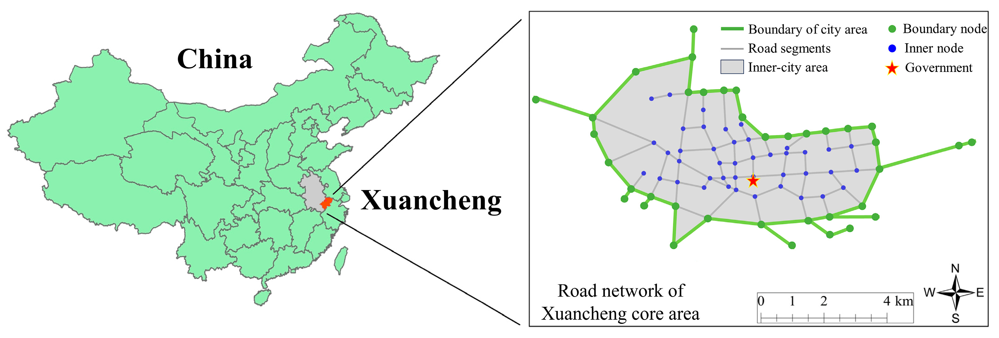
2.1. Study Area and Data Sources

We selected the core area of Xuancheng (Figure 1) as the study area for several key reasons. First, Xuancheng is one of the 27 central cities in the Yangtze River Delta, representing a typical example of China’s rapidly growing small- and medium-sized cities. Xuancheng had a permanent population of 2.64 million in 2018, and the GDP growth rate averaged 10.5% annually from 2005 to 2018. Cities of this scale are critical to promoting sustainable urban development [34]. Second, the vehicle ownership rate in Xuancheng is 0.15 vehicles per capita, closely aligning with the national average of 0.166 vehicles per capita [35]. Third, the core area of Xuancheng features a typical organic grid road network with a boundary ring road and centrally located governmental buildings. This is one of the most common urban road network configurations [36]. Fourth, the extensive deployment of ALPR detectors across the study area provides comprehensive vehicle data for this research and serves as a model for implementing similar methods in other cities.

ALPR detectors are strategically installed at intersections throughout the urban road network (Figure 1), with their locations classified into two categories: boundary nodes (marked in green) and inner nodes (marked in blue). The lines linking boundary nodes define the city boundaries, and the gray area is the inner-city area, which was the study area. Most of the points of interest (POIs) in Xuancheng are concentrated in this area (Figure S1). By using travel origin/destination node classifications, we analyzed the behaviors of vehicles entering and exiting the boundary of the study area. For example, vehicles entering the boundary are likely drawn to the POIs within the study area, while vehicles exiting the boundary suggest that they are traveling to other areas for residential or work-related purposes.

The data source of the comprehensive vehicle travel data was derived from ALPR records. A vehicle passing an ALPR detector triggers the creation of a data record, as detailed in

Table 1. Examples of ALPR records data.

Index	ALPR Location ID	Vehicle ID (Anonymized)	Recording Time
1	XC-01	964352156	30 May 2018/08:00:01
2	XC-02	964352157	30 May 2018/09:00:02

. These records enable the reconstruction of individual driving trajectories, providing comprehensive individual vehicle travel data (Section 2.2). By combining vehicle travel data with a vehicle emission model, we can quantify emissions from individual vehicles (Section 2.3) and construct the UTEFN (Section 2.4). The ALPR dataset used in this study contained approximately 30 million records collected from more than 50,000 vehicles during May 2018.

2.2. Vehicle Travel Data Extraction

Vehicle travel data included vehicle kilometers travelled (VKTs), routes trajectory, times, and corresponding velocities. In this study, a complete instance of travel was defined as a “trip chain” which consisted of several consecutive “trips”. Each “trip” referred to the movement of a vehicle between two neighboring ALPR detectors. The construction of the urban vehicle travel dataset on the basis of ALPR records involved two main steps: trip data generation and OD identification.

First, the ALPR records were sorted according to the vehicle ID and timestamp. By analyzing the ALPR records, the distance, duration, and corresponding speed of each trip could be obtained for every vehicle. Subsequently, a time threshold method was employed to identify the origin and destination of travel. Specifically, we adopted a 10 min time threshold, following the methodology of Hadavi et al. [37]. If the interval between two trips exceeded this threshold, the vehicle was assumed to have made a substantial stop (e.g., returning home, working, or dining). This stop served as a breakpoint, marking the destination of the previous travel and the origin of the next instance of travel. Using this method, trip data could be segmented into multiple trip chains, each representing a complete instance of travel.

2.3. Emission Quantification

Various models have been developed to estimate vehicle emissions, such as COPERT, MOVES, and International Vehicle Emissions (IVE). COPERT [38] and MOVES [39] were specifically designed based on the technological characteristics and emission standards of European and American vehicles, respectively. In contrast, the IVE model is widely recognized as an effective tool for developing urban traffic emission inventories in developing countries and has been extensively applied in regions such as China [40], India [41], and Ecuador [42]. In this study, urban traffic emissions were quantified using the IVE model following a bottom-up approach. Specifically, emissions were first estimated at the level of individual trips, and the emissions from all consecutive trips were then aggregated to obtain the total emissions associated with a complete instance of travel (trip chain). The formulas for calculating travel emissions are as follows:

$$E_{v,r}={\displaystyle {\sum }_p{E}_{v,r,p}}$$

(1)

$$E_{v,r,p}=L_{v,r,p}\times Q_{v,r,p}$$

(2)

Equation (1) defines $E_{v,r}$, the emissions from travel $r$ by vehicle $v$ (g), which is the sum of emissions from each individual trip $p$ within travel $r$. $E_{v,r,p}$ represents the emissions from trip $p$ within the travel $r$ by vehicle $v$; $L_{v,r,p}$ denotes the distance in trip $p$ (m). $Q_{v,r,p}$ corresponds to the emission factor for trip $p$, determined by the IVE model. The emission factor $Q$ is defined as:

$$Q=B\times {\displaystyle \prod K_w}$$

(3)

where $B$ is the baseline emission factor (g/m), which is determined by the vehicle technical attributes, including vehicle type, emission standard, fuel type, and vehicle age. These attributes were obtained by matching license plates with the local vehicle registration database, which provided data on the vehicle’s license number, vehicle type, weight, fuel type, emission standard, and initial registration date. The definitions of vehicle types are presented in Table S1. The emission standards were recorded as the China 1–5 emission standards, which can be considered equal to the Euro 1–5 emission standards. Based on the above technical attributes, the corresponding base emission factor for each vehicle was determined. $K_w$ is the correction factor indexed by $w$ (dimensionless), which is determined by vehicle operating conditions and other parameters, including the vehicle specific power (VSP), engine stress (ES), fuel quality, inspection and maintenance (I/M) status, temperature, humidity, and altitude. These correction factors were determined based on the methodology outlined by Yu et al. [43]. Detailed settings for vehicle operating conditions and other parameters are provided in the Supplementary Note. The above parameters were input to the IVE model to determine the correction factors.

2.4. Modeling and Characteristic Indicators of the UTEFN

2.4.1. Characteristic Indicators of the UTEFN

(1)

Network establishment and edge weight quantification

In this study, the UTEFN was modeled as a weighted directed graph $G(N,E,W)$ where $N$ is the set of nodes, each representing a specific geographic location that serves as an origin or destination for travel. $E$ is the set of edges, and a directed edge $e_{ij}$ exists if there is travel from node $i$ to node $j$. $W$ is the set of edge weight (EW). $E{W}_{ij}$ measures the emission flow from node $i$ to node $j$ and can be estimated as:

$$E{W}_{ij}={\displaystyle {\sum }_v{\displaystyle {\sum }_{r\in S_{ij}}{E}_{v,r}}}$$

(4)

where $S_{ij}$ is the collection of all travel originating at node $i$ and terminating at node $j$.

(2)

Node weighted degree

The node weighted degree (NW) used in this study represented the total emissions associated with a node, including both incoming and outgoing traffic emission flows. $\mathrm{N}\mathrm{W}$ was defined as the sum of the node weighted in-degree ($N{W}^{in}$) and node weighted out-degree ($N{W}^{out}$), as given in Equations (5)–(7). Zang et al. [44] used NW to define the passenger flow strengths of metro stations. Our study expanded this framework by redefining $N{W}_i^{in}$ to include all emission flows ending at node $i$ and redefining $N{W}_i^{out}$ to include all emission flows starting at node $i$. Therefore, $N{W}_i$ provided a measure of the total emissions associated with each node.

$$N{W}_i^{in}={\displaystyle {\sum }_{j}E{W}_{ji}}$$

(5)

$$N{W}_i^{out}={\displaystyle {\sum }_{j}E{W}_{ij}}$$

(6)

$$N{W}_i=N{W}_i^{in}+N{W}_i^{out}$$

(7)

(3)

Scaling law of distribution

To more deeply examine the emission patterns in the UTEFN, we investigated and fit the complementary cumulative distribution functions (CCDFs) of NW and EW. Previous studies have shown that many real-world networks adhere to scaling laws characterized by heavy-tailed distributions [45,46], such as the most typical power law [47]. Heavy-tailed distributions are notable because of the high probability of encountering extremely large values in the distribution’s tail, which do not conform to an exponential bound [48]. Considering this, we applied Kello’s method [49] to fit the data with five hypothesized models: exponential, stretched exponential, power law, truncated power law, and lognormal distributions. Importantly, the smallest nonzero value in the dataset was chosen as the starting point $x_{\min }$ for the fitting process. This approach was intended to enable effective investigation of the scaling law of the emission distribution across the entire network.

2.4.2. Structural Indicators of the UTEFN

(1)

Global structural indicators

Besides analysis of emission distribution, an overview of structural properties allows for the exploration of the UTEFN from a global perspective. Global structural measures used in this study included the network density ($ND$), average clustering coefficient ($CC$), average shortest path ($L$), and small-world coefficient ($SC$), as detailed in

Table 2. Global structural indicators for UTEFN.

Measure	Symbol	General Implication
In degree	$d_i^{in}={\displaystyle {\sum }_j{e}_{ji}}$	The number of edges pointing to node $i$.
Out degree	$d_i^{out}={\displaystyle {\sum }_j{e}_{ij}}$	The number of edges from node $i$ to other nodes.
Degree	$d_i^{tot}=d_i^{in}+d_i^{out}$	The number of edges that are in contact with node $i$.
Bilateral edges number	$d_i^{\leftrightarrow }={\displaystyle \sum _{i\ne j}{e}_{ij}{e}_{ji}}$	The number of nodes $j$ for which both an $e_{ij}$ and an $e_{ji}$ exist.
Network density	$ND={\displaystyle \frac{m}{n^2}}$	The network density between nodes in the network is defined as the ratio of the total number of edges $m$ to the maximum possible number of edges, which is $n^2$, where $n$ represents the number of nodes in the network.
Clustering coefficient	$C{C}_i={\displaystyle \frac{{\left[W^{[1/3]}+{\left(W^T\right)}^{[1/3]}\right]}_{ii}^3}{2\left[d_i^{tot}\left(d_i^{tot}-1\right)-2d_i^{\leftrightarrow }\right]}}$	The clustering coefficient quantifies the level of cohesiveness among the neighbors of a node. In this context, $W$ refers to the edge weight matrix, with ${[W]}_{ii}$ representing the value on the diagonal corresponding to node $i$.
Average clustering coefficient	$CC={\displaystyle \frac{1}{n}}{\displaystyle {\sum }_{i}C{C}_i}$	The mean value of the clustering coefficient for all nodes in the network, $n$ is the total number of nodes in the network.
Average shortest path	$L={\displaystyle \frac{1}{n(n-1)}}{\displaystyle {\sum }_{i\ne j}{l}_{ij}}$	The arithmetic mean of the number of edges in the shortest paths between all pairs of nodes. Where $l_{ij}$ represents the shortest path between node $i$ and $j$, and $n$ is the total number of nodes in the network.
Small-world coefficient	$SC={\displaystyle \frac{CC/C{C}_r}{L/L_r}}$	$CC$ and $C{C}_r$ represent the average clustering coefficient of the UTEFN and an equivalent random network, respectively. $L$ and $L_r$ represent the average shortest path length of the UTEFN and an equivalent random network, respectively.

. Among them, $ND$ indicates the sparsity or compactness of the network. $CC$ reflects the tightness of connections within the network structure [50,51]. $L$ indicates the accessibility between nodes [52]. $CC$ and $L$ can indicate small-world properties in a network [53]. A small-world coefficient greater than one suggests the potential for significant heterogeneity within the network. This heterogeneity may manifest as an uneven distribution of $NW$ and $EW$, with nodes tending to form tightly connected clusters.

(2)

Community structure detection

In network analysis, a community refers to a group of nodes that are closely connected and that exhibit local clustering. This close connection is related to the edges between nodes rather than the attributes of the nodes, as in many traditional clustering methods [54]. Community detection algorithms have gained increasing attention in clustering studies of such traffic systems, which are crucial for urban traffic planning [55,56,57,58]. Therefore, our study used emissions as edge weights to detect communities in the UTEFN to reveal aggregation patterns of emission flows. Specifically, there are more emission flows within a community and fewer emission flows between different communities.

Most community detection algorithms begin by defining a quality function to evaluate the effectiveness of graph partitioning. Modularity is a widely recognized quality function [54]. However, modularity optimization is an NP-hard problem, and it is usually solved via heuristic algorithms. We applied a greedy optimization method proposed by Lu et al., a modified Louvain algorithm [59,60], to discover the highest-quality community classification in the network.

3. Emission Characteristics

This section provides an in-depth analysis of the emission characteristics of the Urban Traffic Emission Flow Network (UTEFN). First, we identified emission peak hours and high-emission road segments using the traditional on-road perspective, which served as a comparison for the network perspective analysis. Subsequently, we examined the emission characteristics from a network perspective, focusing on nodes and edges. Lastly, we explored the scaling law of emission distribution within the UTEFN. The analysis was based on urban traffic emission patterns from a typical weekday (30 May 2018), focusing on key gas categories and vehicle types that significantly impact the urban environment. The IVE model can quantify the emissions of multiple gases, with a focus on carbon dioxide (CO₂) and nitrogen oxides (NO_x). CO₂ is the primary greenhouse gas contributing to long-term global climate change, whereas NO_x adversely affect urban air quality and are linked to various respiratory diseases and environmental issues. In terms of vehicle types, cars (private cars) and trucks emerged as the dominant contributors to traffic emissions in the study area. Cars ranked first in CO₂ and NO_x emissions, accounting for 57.5% and 22.7%, respectively; while trucks, being only 3.7% of the vehicles, contributed 19.1% of NO_x emissions, ranking second (Figure S2). Other research results also show that these two vehicle types are often the largest contributors to urban traffic emissions [61,62]. Accordingly, the present analysis centered on emissions from cars and trucks.

3.1. Emission Characteristics of On-Road Vehicles

Building on the methodology outlined in the previous chapter, this study obtained the individual vehicle emission dataset. In terms of vehicle numbers and emissions, the dataset included 39,963 cars and 1895 trucks, and over the course of the typical weekday, 85,803 kg of CO₂ and 33 kg of NO_x were collectively emitted by cars and 5932 kg of CO₂ and 28 kg of NO_x were emitted by trucks. From a temporal perspective (Figure 2), emissions from both cars and trucks were concentrated during the daytime, but with different peak hours. The emissions from cars exhibited a double-peak fluctuation (Figure 2a), peaking at 7–8 h and 17–18 h, with the evening peak being slightly greater. This double-peak fluctuation is usually caused by urban commuting [13]. A localized minimum value of car emissions occurred at 12–13 h, presumably due to reduced activity during the lunch break. In contrast, trucks reached an emission peak at 12–13 h (Figure 2b). The daytime lows in car emissions coincided with the peaks in truck emissions, possibly because truck operations are strategically scheduled to avoid heavy-traffic periods dominated by cars.

From a spatial perspective, emissions exhibited significant variation across different road segments during peak periods, with distinct geographical distribution patterns for high-emission segments for cars and trucks (Figure 3). For cars, high-emission segments were located both in inner-city areas and along boundary roads (Figure 3a,b). Inner-city high-emission segments experienced elevated emissions due to dense concentrations of residential, commercial, and business establishments (Figure S1), which lead to higher car volumes and consequently higher emissions. The boundary also featured high-emission roads, which serve as conduits for intercity travel. For trucks, emissions were generally high on boundary roads (Figure 3c,d). This may be attributed to the specific across-boundary travel of trucks, which will be further explored in Section 3.2.2.

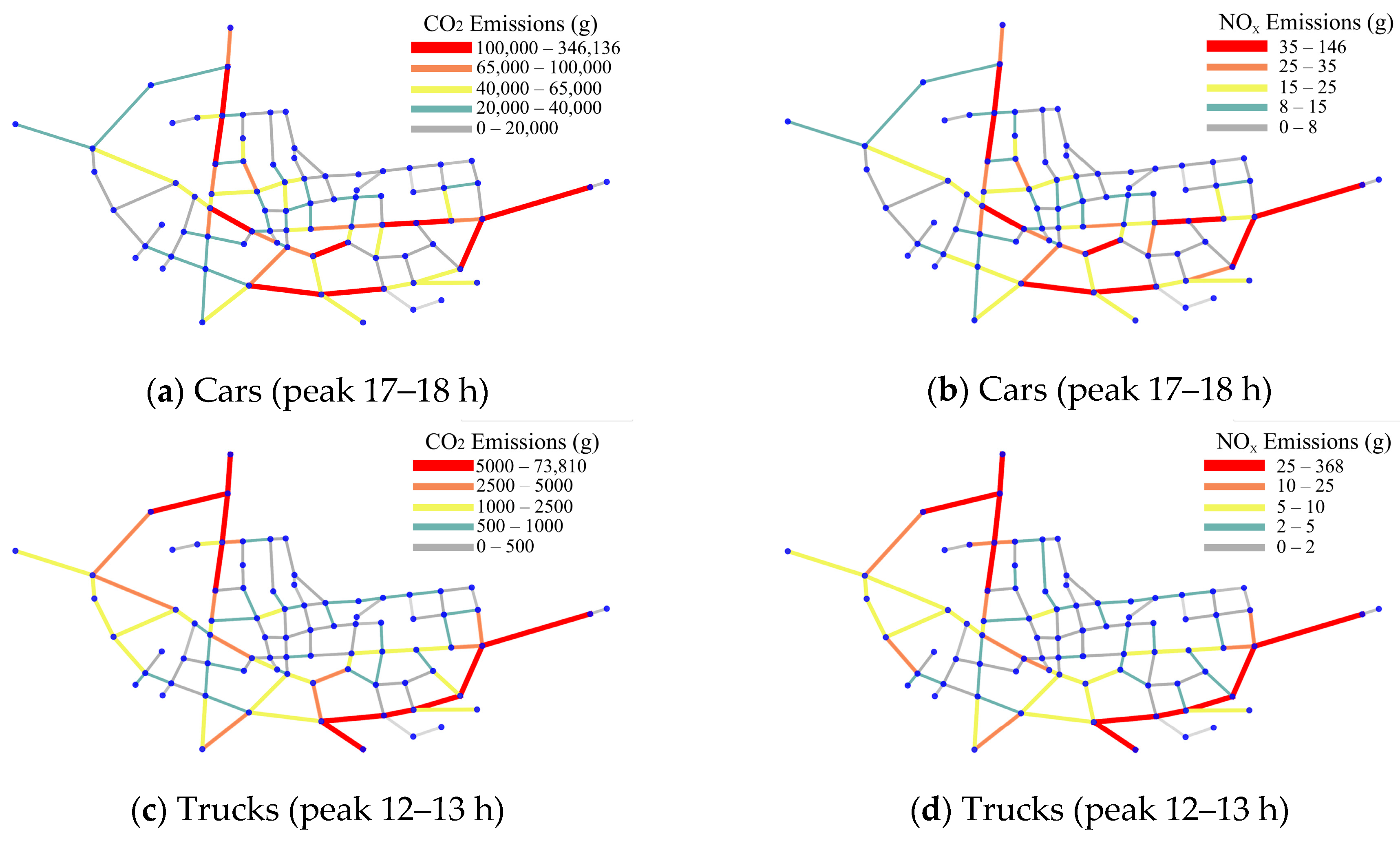
3.2. Emission Characteristics from the Network Perspective

The UTEFN maps traffic emissions onto nodes or edges, as shown in Figure 4. To clearly distinguish vehicle types, we represented the UTEFN for cars as N_C and that for trucks as N_T. This subsection makes an in-depth analysis of the UTEFN from the perspectives of both nodes and edges, and discusses the scaling laws of NW and EW.

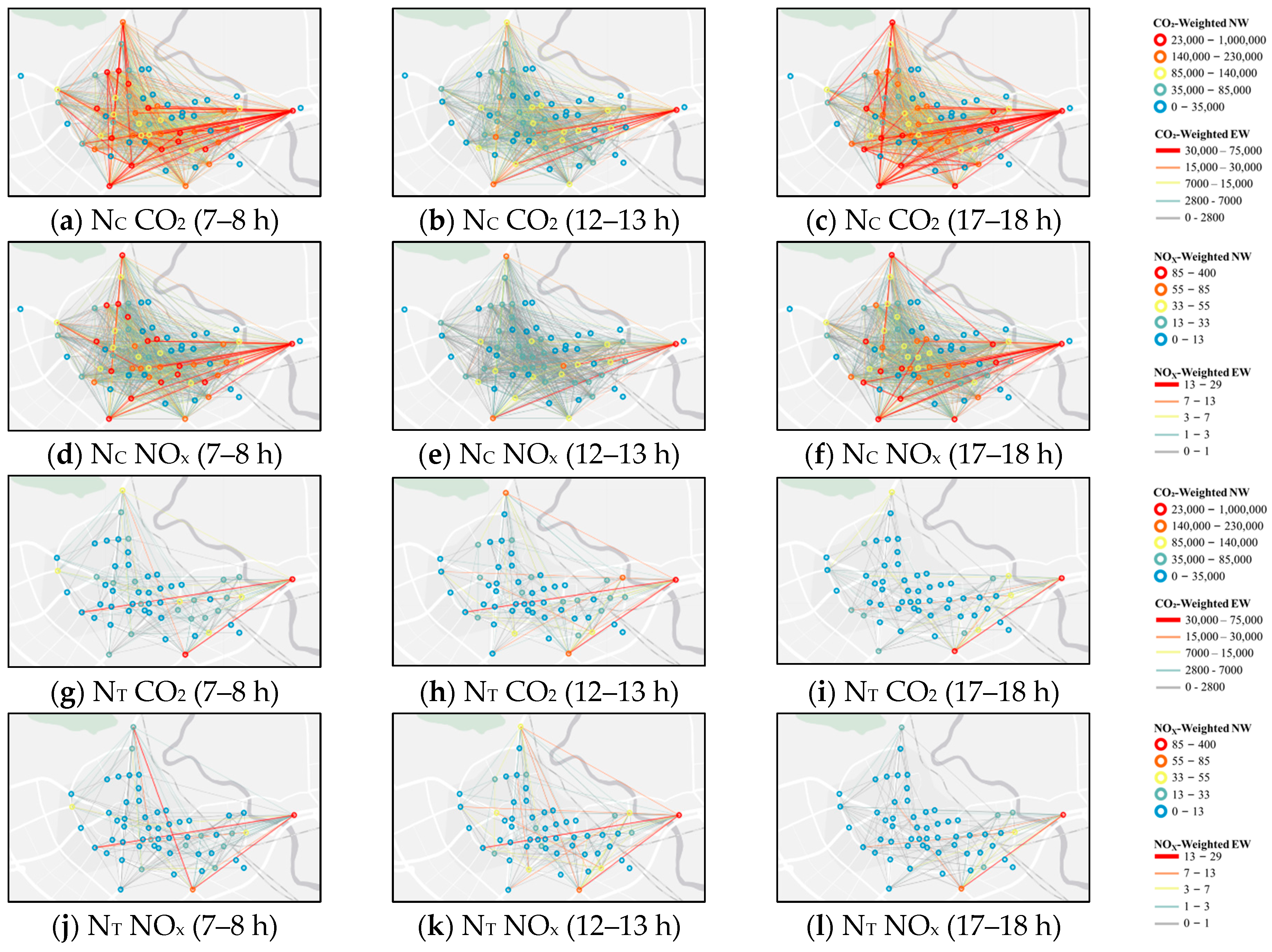
3.2.1. Analysis from the Perspective of Nodes

The NW measures the emissions attributable to nodes that attract and generate travel flows. As shown by the circles in Figure 4a–f, during the peak hours of N_C (7–8 h and 17–18 h), most nodes exhibited significantly higher NW compared to off-peak hours (12–13 h). Conversely, as depicted in Figure 4g–l, N_T nodes showed little variation between daily peak (12–13) and off-peak (7–8 and 17–18) hours, and high NW nodes were predominantly clustered on boundary roads.

The spatial distribution of NW values yields new insights for emission pattern analysis that are not provided by the traditional road-based perspective. Figure 5 presents the high-emission segments (top 10 emission segments) and the high-NW nodes (top 10 NW nodes). The analysis revealed two types of associations between the high-NW nodes and the high-emission segments: connected and separated. On the one hand, some high-NW nodes served as endpoints connecting high-emission road segments, as illustrated by node A in Figure 5a,b. These nodes not only experienced significant traffic emissions but also contributed substantially to overall emissions by attracting and generating large emission flows. On the other hand, there were separated high-NW nodes that were not directly linked to high-emission road segments, such as node B and node C in Figure 5a–d. These nodes were in subregions that did not produce high traffic emissions locally; however, they still significantly contributed to total emissions by attracting and generating large emission flows. Moreover, some separated high-emission road segments without high-NW nodes as endpoints, such as segment A in Figure 5a–d, served as critical hubs connecting key urban areas. Their high emissions were driven more by through-traffic volume than by land use or POIs along the road. Therefore, when managers formulate transportation emission reduction policies, they should consider not only the emissions of vehicles that pass through each area but also the contributions of the areas that attract and generate emission flows.

3.2.2. Analysis from the Perspective of Edges

The emission flow accompanied by travel flow along an OD edge determines the EW. The visual analysis depicted in Figure 4 revealed a marked increase in high-EW edges during peak traffic times for both N_C and N_T. High-EW edges predominantly had an east-west orientation and were frequently associated with boundary nodes. Specifically, for N_C, it was typical for one endpoint of such a high-EW edge to be a boundary node. For N_T, it was common for both endpoints of a high-EW edge to be boundary nodes.

These observations underline the pivotal role of boundary-associated edges in the UTEFN. To examine this role more closely, we categorized the OD edges into four types (Figure 6a), reflecting the four behaviors of vehicle travel: inner-boundary, outbound, inbound, and cross-boundary. In an inner-boundary edge, both the origin and destination nodes were inner-city nodes. Outbound edges extended from inner-city nodes to boundary nodes. Inbound edges linked boundary nodes to inner-city nodes. Cross-boundary edges were defined by having boundary nodes as both origin and destination nodes. For N_C, inner-boundary edges were the predominant contributors to CO₂ and NO_x emissions (Figure 6b,c), accounting for 43% and 40%, respectively. Although these edges did not have distinct red high-EW markings, their density suggested that they made significant emission contributions. The outbound and inbound edges of N_C exhibited peak emissions during the morning and evening rush hours, respectively, highlighting the substantial impact of intercity commuting on urban traffic emissions. Cross-boundary edges contributed the least to emissions, indicating that cross-boundary behavior of cars results in less emissions. Conversely, N_T emissions were primarily from cross-boundary edges, comprising 49% of CO₂ and 54% of NO_x emissions, whereas the emissions of other edge types were comparatively minor (Figure 6d,e). This explains why the high-emission segments for trucks were concentrated at the edges, as noted in Section 3.1. These trucks utilized the study area as a transit route rather than as a real destination or origin, but they significantly influenced the overall urban emission landscape. In summary, emissions for different types of vehicles and edges vary significantly, and comprehensive emission reduction policies are needed to address these disparities.

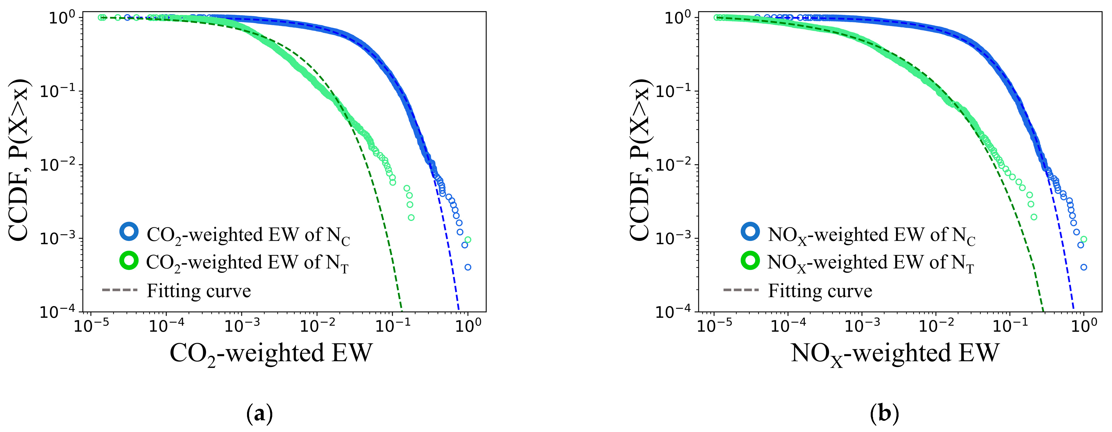
3.2.3. Scaling Laws in the UTEFN

We plotted and fit the CCDFs of NW and EW to explore the scaling laws in the UTEFN (Figure 7 and

Table 3. Fitting parameters normalized EW.

	EW for CO2	EW for NOx
NC	$\lambda$ = 22.06, $\beta$ = 0.79; R2 = 0.997	$\lambda$ = 26.42, $\beta$ = 0.75; R2 = 0.997
NT	$\lambda$ = 232.75, $\beta$ = 0.65; R2 = 0.947	$\lambda$ = 499.08, $\beta$ = 0.470; R2 = 0.990

Note: R² indicates the goodness-of-fit, with values closer to 1 representing a better fit.

). We attempted to fit the CCDFs via five classic heavy-tailed distribution functions. The results indicated that the NW distribution had a heavy-tailed effect. But none of the hypothesized models accurately fit the entire CCDF of NW (Table S2). This suggests that different regions of the NW may present different statistical properties, with poor fits in the beginning and middle regions, but the tail conforms to the power law behavior (Figure S3).

Regarding the edge term, the CCDFs of EW in N_C and N_T displayed heavy-tailed characteristics and could be fitted by multiple hypothesized models (Figure S3). The stretched exponential distribution had the best overall fit (Table S3). The stretched exponential function was formulated as $P(x)\propto x^{(\beta -1)}\exp (-\lambda x^{\beta })$, where $\lambda$ is the scale parameter. A larger $\lambda$ indicates greater volatility in EW distribution, i.e., some edges have extremely high EW values, while others have much lower ones. The parameter $\beta$ is the stretching parameter, reflecting the decay rate of the EW distribution. A smaller $\beta$ suggests a heavier tail, i.e., a higher frequency of extremely high EW values.

Figure 7a shows the fit for CO₂ emissions. The fitted N_T curve showed greater volatility and a slower decline, indicating a more heterogeneous CO₂ EW distribution in N_T. Similarly, the stretched exponential model adequately captured the distribution of NO_x-weighted EW (Figure 7b). Compared with CO₂, NO_x EW had even higher $\lambda$ and smaller $\beta$, indicating that the distribution of NO_x EW was more uneven than that of the CO₂ EW. The statistics also supported this point. The top 10% of the OD edges contributed 40% and 70% to the CO₂ emissions in N_C and N_T, respectively, and 45% and 89% to the NO_x emissions. In summary, both the NW and EW distributions exhibited heavy-tail characteristics, with the scaling laws of the EW distribution accurately captured by a stretched exponential function. This indicates that targeting OD edges with extremely high EW values may significantly enhance the effectiveness of emission reduction policies.

4. Structural Analysis of the UTEFN

4.1. Global Structure of the UTEFN

In addition to analyzing emission distribution, the exploration of network structure can help policymakers gain a deeper understanding of the UTEFN. The global topological measures of the UTEFN are detailed in

Table 4. Network global indicators for UTEFN.

UTEFN	Number of Nodes	Number of Edges	Network Density	Average Shortest Path Length	Average Clustering Coefficient	Small World Metric
NC	75	2470	0.44	1.46 (1.55 *)	0.78 (0.455 *)	1.38
NT	60	1046	0.29	1.7 (1.78 *)	0.51 (0.29 *)	1.83

* Measurements obtained through equivalent random network.

. N_C and N_T had similar numbers of nodes, but N_C had nearly twice as many edges as N_T, leading to a significant difference in network density. This observation suggests that while the OD nodes of N_C and N_T overlap to a high degree within a city, the travel routes of cars are more varied and numerous, whereas those of trucks are more fixed. The average path lengths for both networks were less than two, indicating that on average, no more than two trips were needed to connect any pair of nodes. This metric indicates a high degree of efficiency for both networks. Moreover, the clustering coefficients for both N_C and N_T exceeded those observed in associated randomized networks, reflecting a high density of localized links. In addition, despite their differing scales, both N_C and N_T exhibited the small-world phenomenon (small-world coefficient > 1), which is characterized by efficient connectivity and a substantial clustering trend. To better understand this clustering trend in the network structure, we explored the organizational structure of the UTEFN on the basis of the community discovery algorithm, as discussed in the next section.

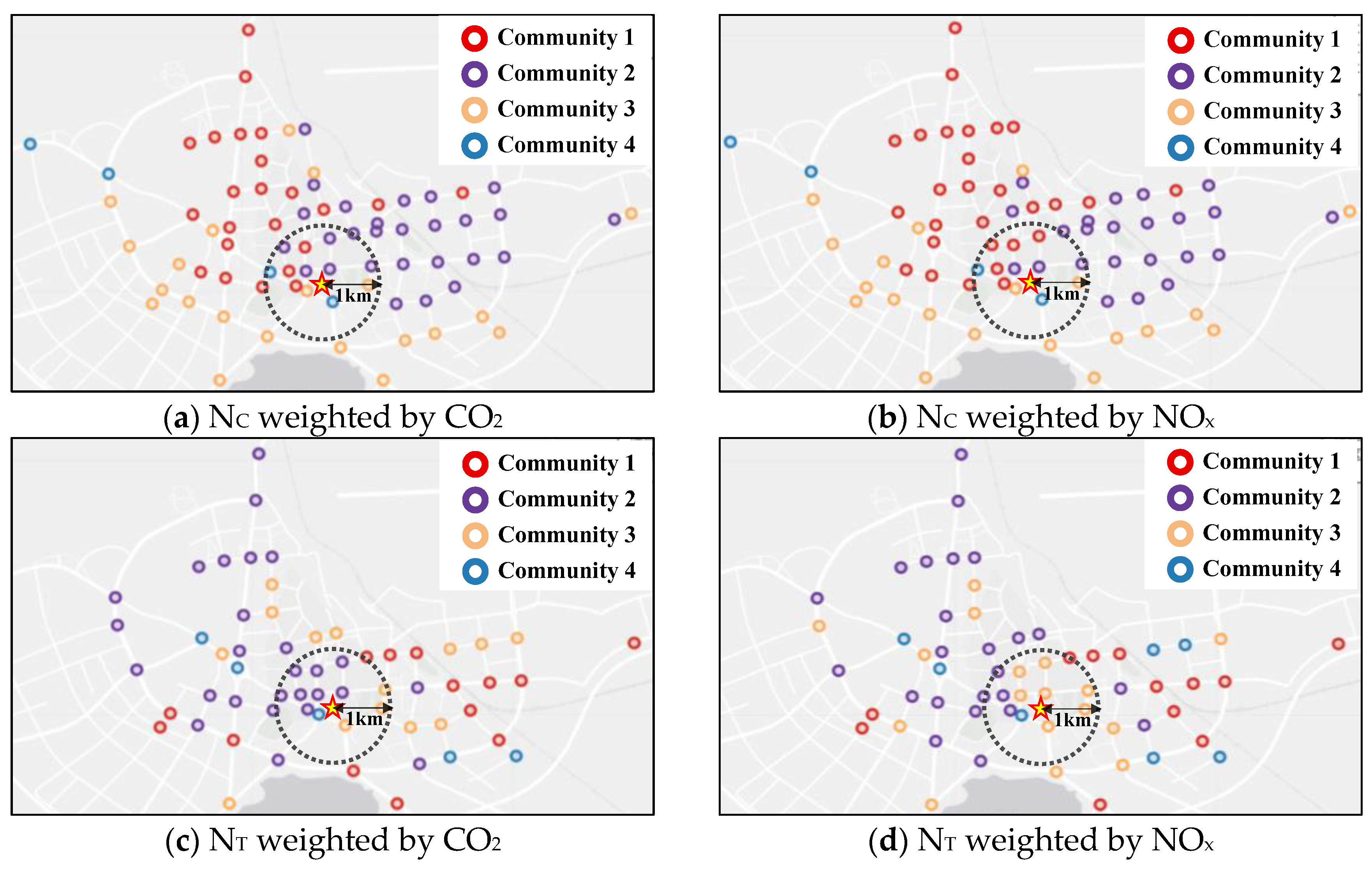
4.2. Structural Analysis of Network Communities

Community structure plays a crucial role in the organization of complex networks, reflecting the local clustering of nodes based on edge connections. We used modularity and Louvain algorithms to detect communities in the UTEFN. After multiple iterations, the optimal modularity values of N_C community classification with CO₂ and NO_x as weight were determined to be 0.17 and 0.18, respectively, while those of trucks were 0.22 and 0.24. A modularity value greater than zero indicates that a significant community structure has been identified in the UTEFN, which suggests that node groupings based on EW show meaningful clustering patterns. Figure 8 illustrates the geographical distribution of community members of N_C and N_T, where the same color represents the same community.

Figure 8a details the division of N_C into four distinct communities on the basis of CO₂ emissions. Community 1, in the northwest, had the highest emission levels and accounted for 49% of the total CO₂ emissions within communities. Community 2, in the northeast, ranked second in terms of emission volume. Community 3 was in the south and had the third largest amount of emissions, with most of its nodes distributed along the boundary roads. Community 4 had the lowest emissions and was more scattered. The variation in emissions across communities may be attributed to the urban spatial configuration. A large number of POIs were concentrated near the internal nodes of Community 1, leading to a high volume of car travel between POIs and consequently higher traffic emissions (Figure S1); the other three communities had fewer POIs and lower emissions. In addition, the algorithm does not impose adjacency constraints, suggesting that the geographical proximity was a fundamental characteristic of the communities in N_C. The black circle centered on the city government in Figure 8a intersects all four communities, highlighting its central role in the urban structure.

Figure 8b presents the community structure obtained by applying the NO_X-weighted algorithm. Despite minor differences in the sizes and shapes of the communities compared with those in Figure 8a, the overarching spatial arrangement at the city scale remained consistent. First, Community 1, again in the northwest, continued to exhibit the highest emissions, accounting for 47% of total NO_x emissions. Second, both Figure 8a,b were divided into four parts, and significant adjacency was observed within these communities. Third, owing to the monocentric urban structure, the city center included members of four communities.

Figure 8c,d show the division of N_T. The community with the highest emissions in N_T was near the city’s southwest corner and was responsible for 61% (CO₂) and 63% (NO_x) of the total emissions. As analyzed in Section 3.2, this can be attributed to a high volume of trucks traversing this area; there was a concentration of high-EW edges in the southwest. The spatial distribution of nodes in the community was not as dense as that in N_C. The reason for this is simple: trucks generally travel longer distances. In addition, the dark circle in the center does not intersect the neighborhoods with the highest emissions, suggesting that the high density of POIs in the city center had limited appeal for trucks.

5. Discussion

5.1. Key Findings

Vehicles generate emissions during movement, creating traffic emission flows between various locations in the city. These flows form a complex system, yet the existing literature lacks a systematic analysis of the emission patterns of such a system. This study introduces a new framework for analyzing urban traffic emission patterns, including comprehensive vehicle travel emission quantification based on ALPR data and emission pattern analysis based on complex network theory. The key findings are as follows:

(1) Emission quantification serves as the foundation for understanding emission patterns. Using ALPR data from Xuancheng, we constructed a comprehensive individual vehicle travel emission dataset and analyzed the emission characteristics of different vehicle types based on the traditional road-based perspective. Specifically, cars, due to their high volume and frequent use, generated significantly more CO₂ emissions compared to trucks; in contrast, trucks exhibited disproportionately high NO_x emissions because diesel fuel—characterized by longer carbon chains and higher combustion temperatures—promotes NO_x formation, resulting in NO_x emission factors up to 35 times those of gasoline cars (see Table S4). The daily emissions of cars exhibited bimodal curves, peaking during morning and evening commuting hours, whereas truck emissions were concentrated during daytime hours. High-emission road segments for cars were concentrated within inner-city road segments, reflecting the influence of residential and commercial POIs. Conversely, trucks played a dominant role in intercity freight, resulting in higher emissions along boundary roads. These findings align with emission quantification studies conducted in other cities [63,64], suggesting common urban traffic emission patterns and supporting the reliability of our estimated results.

(2) From the node perspective, we identified high NW nodes that contribute a lot to urban traffic emissions. On the one hand, some high NW nodes are adjacent to high-emission road segments, and these nodes are usually located near densely populated POIs or serve as entrances and exits. On the other hand, there are discrete high-NW nodes that, although not adjacent to high-emission road segments, significantly increase citywide emissions by attracting or generating large amounts of traffic, possibly due to specific POIs surrounding the nodes (e.g., hospitals and transportation stations). These emission-critical nodes may be overlooked under traditional road-based perspectives pattern analyses, but they play a structurally important role in shaping urban traffic emissions.

(3) From edge perspective, EW of edges highlighted the contribution of OD edges corresponding to different travel behaviors. For cars, the primary emissions originated from inner-city travel, but intercity travel (including inbound, outbound, and cross-boundary travel) still accounted for more than half of the total car emissions. For trucks, cross-boundary travel contributed the majority of emissions. Trucks use Xuancheng as a transit area on their transport routes, rather than as the actual origin or destination, but their transport activities through the city have a significant impact on the city’s overall emissions. These findings highlight the varying roles of travel behaviors in driving urban traffic emissions.

(4) While previous studies have demonstrated that the distribution of road and vehicle emissions in urban networks adheres to scaling laws modeled by truncated power law functions [14], this study innovatively found that the scaling law of EW distribution conforms to a stretched exponential function. This pattern is characterized by a small number of edges generating disproportionately high emissions, which broadens the empirical understanding of scaling laws and heavy-tailed distributions.

(5) The network structure of the UTEFN exhibited small-world characteristics and was partitioned into distinct communities. The high-emission community for cars was concentrated in the POI-dense northwestern areas, while the high-emission community for trucks was located near southeastern boundary roads. This observation indicates spatial segregation in emission flows, similar to the spatial isolation observed in travel flows, showing that zoning control has the potential to effectively reduce traffic emissions.

In summary, the network-based approach provides novel insights distinct from traditional perspectives, enhancing our understanding of urban traffic emission patterns and offering a robust foundation for devising effective emission reduction strategies.

5.2. Practical Implications

The key findings from the network perspective provide information that cannot be discovered from the traditional road perspective and offer insights for developing more comprehensive and long-term traffic emission reduction strategies.

For CO₂ emissions, since cars are responsible for the majority of total CO₂ emissions compared to trucks and other vehicle types, they should be prioritized in urban mitigation strategies. From a traditional perspective, high-emission segments for cars are mainly located along inner-city road segments. From a network perspective, our analysis reveals that more than half of car-related emissions are generated by intercity travel. Based on these findings, in the short term, cities can implement traffic restrictions on high-emission road segments and increase electric bus capacity on high-emission OD edges, especially those associated with intercity travel, in order to partially substitute private car usage. In the medium to long term, reducing the formation of high-emission OD edges requires optimizing urban functional layouts and new energy infrastructure. For example, improving the land-use mix and job–housing balance can shorten passenger mileage; developing efficient intercity roads can enhance travel speed and reduce congestion; and expanding electric vehicle charging infrastructure along high-emission nodes and OD edges can improve electric vehicle convenience and penetration.

For NO_x emissions, trucks as gross polluters primarily generate their emissions from cross-city OD edges. In addition, traditional road-based analysis shows that high-emission road segments for trucks are primarily located along the boundaries of the study area. Based on these findings, in the short term, restricting truck access to urban roads during peak periods can reduce inner-city emissions. At the same time, traffic signal coordination along routes corresponding to high-emission OD edges should be optimized by increasing green wave coverage, thereby reducing emissions caused by stop-and-go driving conditions for trucks. In the medium to long term, regional freight network optimization and the deployment of supporting infrastructure for new energy trucks should be prioritized. For example, developing dedicated urban freight corridors or intercity rail lines; constructing freight transfer hubs to improve freight consolidation efficiency; and deploying hydrogen refueling stations and electric trailer swap stations at high-emission nodes and OD edges to facilitate the large-scale adoption of new energy trucks.

Moreover, based on the scaling law analysis results of nodes and edges in the emission network, it is shown that a few high-emission OD edges and nodes play a dominant role in the overall emissions. Prioritizing emission reduction measures for these critical nodes and edges can greatly improve the efficiency and cost-effectiveness of emission control policies.

In addition, community structure analysis for the UTEFN reveals the spatial patterns of emission flow clusters, providing decision makers with boundary references and priority targets for the differential management of traffic emission zones. It is recommended that policymakers implement targeted interventions in high-emission communities by applying the above-mentioned strategies—such as transit substitution, access restrictions for trucks, and deployment of clean energy infrastructure—specifically to the high-emission OD edges within those communities.

In summary, the network-based approach offers new insights into the spatial interactions and emission characteristics of urban travel and serves as an effective complement to traditional methods. It can support the development of more comprehensive, targeted, and sustainable traffic emission reduction policies.

5.3. Uncertainty Discussion

Uncertainty is unavoidable in emission quantification, particularly in the context of urban traffic emissions, where the main sources of uncertainty arise from vehicle travel data and emission factors.

Regarding vehicle travel data, this study reconstructed speed variation in vehicle travel using data from the ALPR system and employed this information to match the corresponding emission factors. However, due to the ALPR system’s inability to capture instantaneous speed, the average speed over each road segment was used to obtain vehicle operating conditions. According to the study conducted by Choi et al. [65], emissions estimated using average speed are approximately 23% lower than those estimated using instantaneous speed.

With regard to emission factors, this study employed the IVE model to quantify emissions during vehicle operation. According to the findings of Gao et al., when comparing IVE-estimated emission factors with those obtained from direct measurements, the estimated uncertainty range is approximately 5% to 10% [66].

In addition, due to data limitations, this study did not incorporate emission estimates for motorcycles. Therefore, applying this methodology to estimate emissions for entire urban on-road traffic emissions may introduce additional uncertainties. Based on the existing literature, CO₂ and NO_x emissions from motorcycles in China account for approximately 15% and 17%, respectively, of the emissions from private vehicles [67,68].

Despite there being some uncertainties in emission quantification, these are still within the acceptable range for the purpose of revealing the emission patterns of urban traffic.

5.4. Limitations and Future Studies

While this study presents a quantitative analytical approach for understanding the UTEFN, it has several limitations. The case study primarily focuses on two representative vehicle types: cars and trucks. Future work will expand this analysis by integrating other vehicle types (e.g., buses, motorcycles, and mopeds) and pollutants (e.g., NO, NO₂, O₃, and VOCs) to create a more comprehensive UTEFN. Importantly, using ALPR data enables fuel type identification, and as electric vehicle adoption increases in the future, this will allow zero emissions to be assigned to electric vehicles without altering the model structure or logic. This study reconstructed vehicle trajectories and operating condition changes based on a dense ALPR system in Xuancheng. However, the method has not yet been extended to regions with sparse ALPR coverage. It also does not incorporate vehicle-type-specific driving cycles, and actual travel paths may deviate from the shortest-path assumption due to route randomness and traffic conditions. Current research shows that travel trajectories can still be effectively reconstructed as long as the ALPR coverage rate is not less than 40% [69]. Future research will explore more advanced trajectory reconstruction methods, incorporate real-time traffic data, model path variability, and develop driving cycles tailored to different vehicle types. These efforts will enhance model applicability and enable comparative analyses across cities with diverse scales and development stages. In addition, measurements are essential for validation. Although the IVE model has been widely applied and validated [70,71], further local calibration using PEMS data remains important to enhance emission factor accuracy.

6. Conclusions

In this paper, a methodological framework was developed to analyze urban traffic emission patterns from a network perspective. The emissions of individual vehicles in a city were accurately quantified via fine-grained, real-time ALPR data. Complex network theory was subsequently employed to analyze the UTEFN in depth, with a focus on its emission characteristics and network structure. Using the core urban area of Xuancheng as a case study, we analyzed the CO₂ and NO_X emission patterns of both cars and trucks. The main conclusions are as follows: (1) Although some nodes were located far from high-emission road segments, they contributed significantly to the overall traffic emissions because of the traffic flows they attract and generate—an aspect overlooked in prior studies. (2) Intercity emission reduction strategies hold substantial potential to mitigate urban emissions, as over half of car emissions originate from intercity travel, and truck emissions mainly stem from cross-city travel that merely pass through Xuancheng without starting or ending there. (3) Scaling law analysis reveals a heavy-tailed distribution of emissions on OD edges, best fitted by a stretched exponential function, with the top 10% of OD edges contributing an average of more than 60% of total emissions, suggesting that targeted control could significantly enhance emission reduction efficiency. (4) Community detection using the Louvain algorithm effectively reveals local clustering patterns in car and truck emission flows, providing a scientific basis for delineating control zones and prioritizing interventions to support more spatially differentiated emission control.

The main contributions of this study are as follows: (1) This study provides a modeling and analysis framework to reveal urban traffic emission patterns from a network perspective. (2) By leveraging ALPR technology to capture detailed vehicle travel data and parameters, we provide a method for accurately quantifying the emissions of individual vehicles, thereby obtaining a more precise depiction of emission patterns. The network perspective provides new insights that can enhance existing emission reduction policies and support the development of sustainable urban traffic solutions.

References

1. International Energy Agency (IEA). Global CO2 Emissions from Transport by Sub-Sector in the Net Zero Scenario, 2000–2030. Available online: https://www.iea.org/data-and-statistics/charts/global-co2-emissions-from-transport-by-sub-sector-in-the-net-zero-scenario-2000-2030-2 (accessed on 8 May 2025).
2. Boogaard, H.; Patton, A.P.; Atkinson, R.W.; Brook, J.R.; Chang, H.H.; Crouse, D.L.; Fussell, J.C.; Hoek, G.; Hoffmann, B.; Kappeler, R.; et al. Long-term exposure to traffic-related air pollution and selected health outcomes: A systematic review and meta-analysis. Environ. Int. 2022, 164, 107262. [Google Scholar] [CrossRef] [PubMed]
3. Khreis, H.; Sanchez, K.A.; Foster, M.; Burns, J.; Nieuwenhuijsen, M.J.; Jaikumar, R.; Ramani, T.; Zietsman, J. Urban policy interventions to reduce traffic-related emissions and air pollution: A systematic evidence map. Environ. Int. 2023, 172, 107805. [Google Scholar] [CrossRef] [PubMed]
4. Fu, X.; Cheng, J.; Peng, L.; Zhou, M.; Mauzerall, D.L. Co-benefits of transport demand reductions from compact urban development in Chinese cities. Nat. Sustain. 2024, 7, 294–304. [Google Scholar] [CrossRef]
5. Deng, X.; Chen, W.; Zhou, Q.; Zheng, Y.; Li, H.; Liao, S.; Biljecki, F. Exploring spatiotemporal pattern and agglomeration of road CO2 emissions in Guangdong, China. Sci. Total Environ. 2023, 871, 162134. [Google Scholar] [CrossRef]
6. Cai, H.; Xie, S. Estimation of vehicular emission inventories in China from 1980 to 2005. Atmos. Environ. 2007, 41, 8963–8979. [Google Scholar] [CrossRef]
7. Kinnee, E.J.; Touma, J.S.; Mason, R.; Thurman, J.; Beidler, A.; Bailey, C.; Cook, R. Allocation of on road mobile emissions to road segments for air toxics modeling in an urban area. Transp. Res. Part D Transp. Environ. 2004, 9, 139–150. [Google Scholar] [CrossRef]
8. Saide, P.; Zah, R.; Osses, M. Spatial disaggregation of traffic emission inventories in large cities using simplified top-down methods. Atmos. Environ. 2009, 43, 4914–4923. [Google Scholar] [CrossRef]
9. Liu, Y.; Ma, J.; Li, L.; Lin, X.; Xu, W.; Ding, H. A high temporal-spatial vehicle emission inventory based on detailed hourly traffic data in a medium-sized city of China. Environ. Pollut. 2018, 236, 324–333. [Google Scholar] [CrossRef]
10. Zhou, Z.; Tan, Q.; Liu, H.; Deng, Y.; Wu, K.; Lu, C.; Zhou, X. Emission characteristics and high-resolution spatial and temporal distribution of pollutants from motor vehicles in Chengdu, China. Atmos. Pollut. Res. 2019, 10, 749–758. [Google Scholar] [CrossRef]
11. Xu, Y.; Liu, Z.; Xue, W.; Yan, G.; Shi, X.; Zhao, D.; Zhang, Y.; Lei, Y.; Wang, J. Identification of on-road vehicle CO2 emission pattern in China: A study based on a high-resolution emission inventory. Resour. Conserv. Recycl. 2021, 175, 105891. [Google Scholar] [CrossRef]
12. Lin, C.; Zhou, X.; Wu, D.; Gong, B. Estimation of Emissions at Signalized Intersections Using an Improved MOVES Model with GPS Data. Int. J. Environ. Res. Public Health 2019, 16, 3647. [Google Scholar] [CrossRef]
13. Tian, D.; Zhang, J.; Li, B.; Xia, C.; Zhu, Y.; Zhou, C.; Wang, Y.; Liu, X.; Yang, M. Spatial analysis of commuting carbon emissions in main urban area of Beijing: A GPS trajectory-based approach. Ecol. Ind. 2024, 159, 111610. [Google Scholar] [CrossRef]
14. Böhm, M.; Nanni, M.; Pappalardo, L. Gross polluters and vehicle emissions reduction. Nat. Sustain. 2022, 5, 699–707. [Google Scholar] [CrossRef]
15. Cheng, S.; Zhao, Y.; Zhang, B.; Peng, P.; Lu, F. Structural decomposition of heavy-duty diesel truck emission contribution based on trajectory mining. J. Clean. Prod. 2022, 380, 135172. [Google Scholar] [CrossRef]
16. Shang, W.; Chen, Y.; Yu, Q.; Song, X.; Chen, Y.; Ma, X.; Chen, X.; Tan, Z.; Huang, J.; Ochieng, W. Spatio-temporal analysis of carbon footprints for urban public transport systems based on smart card data. Appl. Energy 2023, 352, 121859. [Google Scholar] [CrossRef]
17. Cai, Y.; Zeng, X.; Li, W.; He, S.; Feng, Z.; Tan, Z. Managing Uncertainty in Urban Road Traffic Emissions Associated with Vehicle Fleet Composition: From the Perspective of Spatiotemporal Sampling Coverage. Sustainability 2024, 16, 3504. [Google Scholar] [CrossRef]
18. Sun, D.; Zhang, K.; Shen, S. Analyzing spatiotemporal traffic line source emissions based on massive didi online car-hailing service data. Transp. Res. Part D Transp. Environ. 2018, 62, 699–714. [Google Scholar] [CrossRef]
19. Zhang, S.; Niu, T.; Wu, Y.; Zhang, K.M.; Wallington, T.J.; Xie, Q.; Wu, X.; Xu, H. Fine-grained vehicle emission management using intelligent transportation system data. Environ Pollut. 2018, 241, 1027–1037. [Google Scholar] [CrossRef]
20. Rao, W.; Wu, Y.-J.; Xia, J.; Ou, J.; Kluger, R. Origin-destination pattern estimation based on trajectory reconstruction using automatic license plate recognition data. Transp. Res. Part C Emerg. Technol. 2018, 95, 29–46. [Google Scholar] [CrossRef]
21. Pereira, G.; Raetzsch, C. From Banal Surveillance to Function Creep: Automated License Plate Recognition (ALPR) in Denmark. Surveill. Soc. 2022, 20, 265–280. [Google Scholar] [CrossRef]
22. Luvizon, D.C.; Nassu, B.T.; Minetto, R. A Video-Based System for Vehicle Speed Measurement in Urban Roadways. IEEE Transp. Intell. Transp. 2016, 18, 1393–1404. [Google Scholar] [CrossRef]
23. Li, R.; Yang, F.; Liu, Z.; Shang, P.; Wang, H. Effect of taxis on emissions and fuel consumption in a city based on license plate recognition data: A case study in Nanning, China. J. Clean. Prod. 2019, 215, 913–925. [Google Scholar] [CrossRef]
24. Dai, Y.; Shi, X.; Huang, Z.; Du, W.; Cheng, J. Proposal of policies based on temporal-spatial dynamic characteristics and co-benefits of CO2 and air pollutants from vehicles in Shanghai, China. J. Environ. Manag. 2024, 351, 119736. [Google Scholar] [CrossRef]
25. Teng, W.; Shi, C.; Yu, Y.; Li, Q.; Yang, J. Uncovering the spatiotemporal patterns of traffic-related CO2 emission and carbon neutrality based on car-hailing trajectory data. J. Clean. Prod. 2024, 467, 142925. [Google Scholar] [CrossRef]
26. Ren, L.; Guo, X.; Wu, J.; Singh, A.K. Data mining and spatio-temporal characteristics of urban road traffic emissions: A case study in Shijiazhuang, China. PLoS ONE 2023, 18, e0295664. [Google Scholar] [CrossRef] [PubMed]
27. Gómez, C.D.; González, C.M.; Osses, M.; Aristizábal, B.H. Spatial and temporal disaggregation of the on-road vehicle emission inventory in a medium-sized Andean city. Comparison of GIS-based top-down methodologies. Atmos. Environ. 2018, 179, 142–155. [Google Scholar] [CrossRef]
28. Cheng, S.; Lu, F.; Peng, P. A high-resolution emissions inventory and its spatiotemporal pattern variations for heavy-duty diesel trucks in Beijing, China. J. Clean. Prod. 2020, 250, 119445. [Google Scholar] [CrossRef]
29. Deng, F.; Lv, Z.; Qi, L.; Wang, X.; Shi, M.; Liu, H. A big data approach to improving the vehicle emission inventory in China. Nat. Commun. 2020, 11, 2801. [Google Scholar] [CrossRef]
30. Tang, J.; McNabola, A.; Misstear, B.; Caulfield, B. An evaluation of the impact of the Dublin Port Tunnel and HGV management strategy on air pollution emissions. Transp. Res. Part D Transp. Environ. 2017, 52, 1–14. [Google Scholar] [CrossRef]
31. Faloutsos, M.; Faloutsos, P.; Faloutsos, C. On power-law relationships of the Internet topology. SIGCOMM Comput. Commun. Rev. 1999, 29, 251–262. [Google Scholar] [CrossRef]
32. Siganos, G.; Faloutsos, M.; Faloutsos, P.; Faloutsos, C. Power laws and the AS-level Internet topology. IEEE ACM T. Netw. 2003, 11, 514–524. [Google Scholar] [CrossRef]
33. Fan, Y.; Khattak, A.J. Urban Form, Individual Spatial Footprints, and Travel: Examination of Space-Use Behavior. Transp. Res. Rec. 2008, 2082, 98–106. [Google Scholar] [CrossRef]
34. Central Committee of the Communist Party of China. State Council. Outline of Regional Integration Development Plan for the Yangtze River Delta. 2024. Available online: https://www.gov.cn/zhengce/2019-12/01/content_5457442.htm (accessed on 8 May 2025).
35. National Bureau of Statistics, P.R.C. China Statistical Yearbook 2019; China Statistics Press: Beijing, China, 2019. [Google Scholar]
36. Cheng, W.; Huang, H.; Liao, S.; Gao, F.; Biljecki, F. Global urban road network patterns: Unveiling multiscale planning paradigms of 144 cities with a novel deep learning approach. Landsc. Urban Plan. 2024, 241, 104901. [Google Scholar] [CrossRef]
37. Hadavi, S.; Rai, H.B.; Verlinde, S.; Huang, H.; Macharis, C.; Guns, T. Analyzing passenger and freight vehicle movements from automatic-Number plate recognition camera data. Eur. Transp. Res. Rev. 2020, 12, 37. [Google Scholar] [CrossRef]
38. Calculations of Emissions from Road Transport (COPERT). EU. Available online: https://copert.emisia.com (accessed on 8 May 2025).
39. MOVES and Mobile Source Emissions Research. USA EPA. Available online: https://www.epa.gov/moves (accessed on 8 May 2025).
40. Peng, T.; Gan, M.; Yao, Z.; Yang, X.; Liu, X. Nonlinear impacts of urban built environment on freight emissions. Transp. Res. Part D Transp. Environ. 2024, 134, 104358. [Google Scholar] [CrossRef]
41. Mishra, D.; Goyal, P. Estimation of vehicular emissions using dynamic emission factors: A case study of Delhi, India. Atmos. Environ. 2014, 98, 1–7. [Google Scholar] [CrossRef]
42. Viteri, R.; Borge, R.; Paredes, M.; Pérez, M.A. A high resolution vehicular emissions inventory for Ecuador using the IVE modelling system. Chemosphere 2023, 315, 137634. [Google Scholar] [CrossRef]
43. Yu, Z.; Li, W.; Liu, Y.; Zeng, X.; Zhao, Y.; Chen, K.; Zou, B.; He, J. Quantification and management of urban traffic emissions based on individual vehicle data. J. Clean. Prod. 2021, 328, 129386. [Google Scholar] [CrossRef]
44. Zeng, J.; Xiong, Y.; Liu, F.; Ye, J.; Tang, J. Uncovering the spatiotemporal patterns of traffic congestion from large-scale trajectory data: A complex network approach. Phys. A 2022, 604, 127871. [Google Scholar] [CrossRef]
45. Lämmer, S.; Gehlsen, B.; Helbing, D. Scaling laws in the spatial structure of urban road networks. Phys. A 2006, 363, 89–95. [Google Scholar] [CrossRef]
46. Chen, D.; Shao, Q.; Liu, Z.; Yu, W.; Chen, C.L.P. Ridesourcing Behavior Analysis and Prediction: A Network Perspective. IEEE Trans. Intell. Transp. Syst. 2022, 23, 1274–1283. [Google Scholar] [CrossRef]
47. Nakamura, T.; Kiyono, K.; Yoshiuchi, K.; Nakahara, R.; Struzik, Z.R.; Yamamoto, Y. Universal Scaling Law in Human Behavioral Organization. Phys. Rev. Lett. 2007, 99, 138103. [Google Scholar] [CrossRef] [PubMed]
48. Clauset, A.; Shalizi, C.R.; Newman, M.E.J. Power-Law Distributions in Empirical Data. SIAM Rev. 2009, 51, 661–703. [Google Scholar] [CrossRef]
49. Kello, C.T.; Brown, G.D.A.; Ferrer-i-Cancho, R.; Holden, J.G.; Linkenkaer-Hansen, K.; Rhodes, T.; Van Orden, G.C. Scaling laws in cognitive sciences. Trends Cogn. Sci. 2010, 14, 223–232. [Google Scholar] [CrossRef] [PubMed]
50. Fagiolo, G. Clustering in Complex Directed Networks. Phys. Rev. E 2007, 76, 026107. [Google Scholar] [CrossRef]
51. Wei, Y.; Song, W.; Xiu, C.; Zhao, Z. The rich-club phenomenon of China’s population flow network during the country’s spring festival. Appl. Geogr. 2018, 96, 77–85. [Google Scholar] [CrossRef]
52. Ganesh, B. Analysis of the airport network of India as a complex weighted network. Phys. A 2008, 387, 2972–2980. [Google Scholar] [CrossRef]
53. Wang, Y.; Deng, Y.; Ren, F.; Zhu, R.; Wang, P.; Du, T.; Du, Q. Analysing the spatial configuration of urban bus networks based on the geospatial network analysis method. Cities 2020, 96, 102406. [Google Scholar] [CrossRef]
54. Zhang, W.; Thill, J.-C. Detecting and visualizing cohesive activity-travel patterns: A network analysis approach. Comput. Environ. Urban Syst. 2017, 66, 117–129. [Google Scholar] [CrossRef]
55. Yang, Y.; Jia, B.; Yan, X.; Zhi, D.; Song, D.; Chen, Y.; de Bok, M.; Tavasszy, L.A.; Gao, Z. Uncovering and modeling the hierarchical organization of urban heavy truck flows. Transp. Res. Part E Logist. Transp. Rev. 2023, 179, 103318. [Google Scholar] [CrossRef]
56. Liu, X.; Gong, L.; Gong, Y.; Liu, Y. Revealing travel patterns and city structure with taxi trip data. J. Transp. Geogr. 2015, 43, 78–90. [Google Scholar] [CrossRef]
57. Lancichinetti, A.; Fortunato, S.; Radicchi, F. Benchmark graphs for testing community detection algorithms. Phys. Rev. E 2008, 78, 046110. [Google Scholar] [CrossRef]
58. Yildirimoglu, M.; Kim, J. Identification of communities in urban mobility networks using multi-layer graphs of network traffic. Transp. Res. Part C Emerg. Technol. 2018, 89, 254–267. [Google Scholar] [CrossRef]
59. Lu, H.; Halappanavar, M.; Kalyanaraman, A. Parallel heuristics for scalable community detection. Parallel Comput. 2015, 47, 19–37. [Google Scholar] [CrossRef]
60. Blondel, V.D.; Guillaume, J.-L.; Lambiotte, R.; Lefebvre, E. Fast unfolding of communities in large networks. J. Stat. Mech. Theory Exp. 2008, 2008, P10008. [Google Scholar] [CrossRef]
61. Teng, W.; Zhang, Q.; Guo, Z.; Ying, G.; Zhao, J. Carbon emissions from road transportation in China: From past to the future. Environ. Sci. Pollut. Res. 2024, 31, 48048–48061. [Google Scholar] [CrossRef]
62. Tian, X.; Huang, G.; Song, Z.; An, C.; Chen, Z. Impact from the evolution of private vehicle fleet composition on traffic related emissions in the small-medium automotive city. Sci. Total Environ. 2022, 840, 156657. [Google Scholar] [CrossRef]
63. Zhu, B.; Hu, S.; Chen, X.; Roncoli, C.; Lee, D.-H. Uncovering driving factors and spatiotemporal patterns of urban passenger car CO2 emissions: A case study in Hangzhou, China. Appl. Energy 2024, 375, 124094. [Google Scholar] [CrossRef]
64. Cheng, S.; Zhang, B.; Zhao, Y.; Peng, P.; Lu, F. Multiscale spatiotemporal variations of NOx emissions from heavy duty diesel trucks in the Beijing-Tianjin-Hebei region. Sci. Total Environ. 2023, 854, 158753. [Google Scholar] [CrossRef]
65. Choi, H.W.; Frey, H.C. Light duty gasoline vehicle emission factors at high transient and constant speeds for short road segments. Transp. Res. D Transp. Environ. 2009, 14, 610–614. [Google Scholar] [CrossRef]
66. Gao, C.; Gao, C.; Song, K.; Xing, Y.; Chen, W. Vehicle emissions inventory in high spatial–temporal resolution and emission reduction strategy in Harbin-Changchun Megalopolis. Process Saf. Environ. Prot. 2020, 138, 236–245. [Google Scholar] [CrossRef]
67. Hao, H.; Geng, Y.; Wang, H.; Ouyang, M. Regional disparity of urban passenger transport associated GHG (greenhouse gas) emissions in China: A review. Energy 2014, 68, 783–793. [Google Scholar] [CrossRef]
68. Tang, G.; Chao, N.; Wang, Y.; Chen, J. Vehicular emissions in China in 2006 and 2010. J. Environ. Sci. 2016, 48, 179–192. [Google Scholar] [CrossRef]
69. Yang, J.; Sun, J. Vehicle path reconstruction using automatic vehicle identification data: An integrated particle filter and path flow estimator. Transp. Res. Part C Emerg. Technol. 2015, 58, 107–126. [Google Scholar] [CrossRef]
70. Wang, H.; Chen, C.; Huang, C.; Fu, L. On-Road Vehicle Emission Inventory and Its Uncertainty Analysis for Shanghai, China. Sci. Total Environ. 2008, 398, 60–67. [Google Scholar] [CrossRef]
71. Yang, X.; Yao, D.; Xu, R.; Pian, Y.; Liu, S.; Liu, Y. Assessment of full-process VOCs emissions of on-road vehicles considering individual parking behaviors. Transp. Res. D Transp. Environ. 2025, 142, 104678. [Google Scholar] [CrossRef]
Figure 1. Study area.
Atmosphere 16 00594 g001
Figure 2. Temporal dynamics of traffic emissions for cars (a) and trucks (b).
Atmosphere 16 00594 g002
Figure 3. Emissions of road segments during peak hours.
Atmosphere 16 00594 g003
Figure 4. Spatiotemporal distribution of NW (node weighted degree) and EW (edge weight) in UTEFN for cars and trucks: (ac) represent NW and EW weighted by CO2 in NC; (df) represent NW and EW weighted by NOx in NC; (gi) represent NW and EW weighted by CO2 in NT; (jl) represent NW and EW weighted by NOx in NT.
Atmosphere 16 00594 g004
Figure 5. Comparison between high-emission segments and high-NW nodes.
Atmosphere 16 00594 g005
Figure 6. Four types of travel behaviors and corresponding edge weight dynamics.
Atmosphere 16 00594 g006
Figure 7. CCDFs of EWs and stretched exponential fitting for (a) NC and (b) NT.
Atmosphere 16 00594 g007
Figure 8. Structures of communities in NC and NT weighted by CO2 and NOX.
Atmosphere 16 00594 g008